CREATING DISASTERS: RECESSION FORECASTING WITH GAN-GENERATED SYNTHETIC TIME SERIES DATA - arXiv
←
→
Page content transcription
If your browser does not render page correctly, please read the page content below
C REATING D ISASTERS : R ECESSION F ORECASTING WITH
                                                      GAN- GENERATED S YNTHETIC T IME S ERIES DATA

                                                                                                   Sam Dannels ∗
arXiv:2302.10490v1 [cs.LG] 21 Feb 2023

                                                                                               Draft: February 2023

                                                                                                   A BSTRACT

                                                      A common problem when forecasting rare events, such as recessions, is limited data availability. Re-
                                                      cent advancements in deep learning and generative adversarial networks (GANs) make it possible
                                                      to produce high-fidelity synthetic data in large quantities. This paper uses a model called Doppel-
                                                      GANger, a GAN tailored to producing synthetic time series data, to generate synthetic Treasury
                                                      yield time series and associated recession indicators. It is then shown that short-range forecasting
                                                      performance for Treasury yields is improved for models trained on synthetic data relative to models
                                                      trained only on real data. Finally, synthetic recession conditions are produced and used to train clas-
                                                      sification models to predict the probability of a future recession. It is shown that training models on
                                                      synthetic recessions can improve a model’s ability to predict future recessions over a model trained
                                                      only on real data.

                                         1       Introduction

                                         One of the most difficult tasks in forecasting and predictive analytics is predicting a rare occurrence event. Events
                                         that occur with low frequency, and thus have low probability in the sample space, are difficult to adequately measure
                                         and incorporate into a model due to a lack of sufficient data. One such event is an economic recession. The National
                                         Bureau of Economic Research (NBER) tasks its Business Cycle Dating Committee with classifying business cycle
                                         peaks and troughs, which indicate the turning points between economic expansions and contractions. NBER classifies
                                         a recession as a time period that "involves a significant decline in economic activity that is spread across the economy
                                         and lasts more than a few months" (2023). Between January 1965 and January 2023, NBER lists only eight recessions.
                                         Perhaps the most famous leading indicator of a recession is an inversion of the yield curve. The yield curve measures
                                         how yields vary for Treasury bills and bonds based on their maturity. Generally, short-term bills will have lower yield
                                         than longer-term bonds. Occasionally, the yield curve will "invert", meaning that market forces have driven short-term
                                         yields above long-term yields. It has been well documented that this phenomenon can be a useful indicator that a
                                         recession is imminent (Bernard & Gerlach, 1998; Estrella & Hardouvelis, 1991; Kessel, 1965), and that utilizing the
                                         spread between short and long-term yields can predict recessions better than many other leading indicators (Estrella
                                         & Mishkin, 1996).
                                         While yield curve inversions may show promise in predicting recessions, difficulty arises in training and testing a
                                         model on the few available recessions for which there is adequate data. In order to better train a model to predict
                                         recessions, one would need to observe more recessions. Recent advances in the ability of generative adversarial
                                         networks (GANs) to create synthetic replicates of time series data may provide a solution to this problem. The goal of
                                         this paper is to demonstrate that generating synthetic replicates of Treasury bond yield data shows initial promise in
                                         improving short-term forecasts of yield movements, as well as strengthens the signal provided by recession probability
                                         models making use of the Treasury yield spread.

                                             ∗
                                                 University of Iowa, Department of Statistics and Actuarial Science. Email: sam.dannels@gmail.com
Creating Disasters: Recession Forecasting with GAN-generated Synthetic Time Series Data
2 Background
2.1 Synthetic Data
Synthetic data is an artificial replicate of a real data example that is ideally drawn from the same distribution as the
original example. Synthetic data can be generated manually by experts or through a statistical or machine learning
algorithm. The resulting synthetic data should have high fidelity, that is it should maintain the statistical properties of
the original example it is based on while not being an exact replicate of the original data (Lin, Jain, Wang, Fanti, &
Sekar, 2020; Nikolenko, 2019).
Synthetic data is useful for the purpose of sharing data for collaboration across organizations without revealing any
proprietary information (Lin et al., 2020), providing more samples or increasing the frequency of novel samples in
a sparse data set (Nikolenko, 2019), and in some cases can increase predictive performance over models trained
on traditional data (Fawaz, Forestier, Weber, Idoumghar, & Muller, 2018; Frid-Adar, Klang, Amitai, Goldberger, &
Greenspan, 2018).
There are many means of producing synthetic data, but the recent success of GANs in producing high-fidelity replicates
of images (Karras, Laine, & Aila, 2018; Zhu, Park, Isola, & Efros, 2017) has led to their popularity among researchers.
One particular GAN that has demonstrated success in producing synthetic samples of multidimensional time series
data is called DoppelGANger (Lin et al., 2020). In this paper, DoppelGANger will be the model used to produce
high-fidelity replicates of 1-year and 10-year Treasury bond yields. Before moving on to the specific architecture of
DoppelGANger, we will review the general structure and training of GANs.
2.2 GANs
GANs were first introduced by Goodfellow et al. in the 2014 work "Generative Adversarial Networks". The following
section is a summary of the ideas proposed in that paper. The basic idea behind the method they introduced is that
there are two models - a generative model, G, and a discriminative model, D - that compete in a minimax game. The
generative model (generator) is given latent variables (noise) as inputs and attempts to produce a mapping from the
latent space to some desired data space. An example would be a generator that produces realistic images of cats. It
would attempt to learn a mapping from the latent space to a complex probability space that represents realistic-looking
photos of cats. The discriminative model (discriminator) is given inputs from both the real data and the fake samples
produced by the generator and tasked with distinguishing between the two. It produces a single probability that the
input came from the data rather than the generator. In our example, the discriminator would provide a probability
that the given input is a real image of a cat and thus not a computer-generated image of a cat. The two models are
trained in an adversarial way, such that the generator seeks to trick the discriminator with its fake samples while the
discriminator seeks to correctly classify each input it is given as real or generated data. The ultimate goal is that this
minimax optimization training scheme will result in a generator that is able to produce high-fidelity samples from the
same space as the original data.
More specifically, allow x to be the data samples for training the GAN and z to be the latent variables provided to the
generator. Then the minimax problem can be represented by:
min max E [logD(x)] + E [log(1 − D(G(z)))]
G D x∼pdata z∼pz
While G and D can be a wide variety of differentiable functions, in practice they are most commonly deep neural
networks. GANs require few assumptions about the data space and can be trained through common backpropagation
algorithms, which avoid the need for difficult parametric likelihood maximization and Markov Chains (Goodfellow et
al., 2014; Lin et al., 2020). In practice, G and D are trained iteratively. D is trained for k steps while G is held fixed,
and then G is trained for a single step while D is held fixed. When updating G, the gradient is computed for both
D and G, because the gradient backpropagation must pass through D, but the weights are only updated for G. k is a
hyperparameter whose optimal value can vary based on the task at hand (Glassner, 2021; Goodfellow et al., 2014).
When training GANs, there are a few extra considerations to improve the chances of convergence. Dropout, the
practice of regularizing a neural network by stochastically dropping nodes throughout the training process, can help
avoid overfitting (Goodfellow, Bengio, & Courville, 2016). To avoid overfitting GANs, it is important to include
dropout in the training process, especially in the discriminator (Goodfellow et al., 2016). It has also been shown that
in practice, training G to maximize logD(G(z)) rather than minimize log(1 − D(G(z))) can improve the efficiency
of training (Goodfellow et al., 2014).
2Creating Disasters: Recession Forecasting with GAN-generated Synthetic Time Series Data
GAN training can be very unstable. GANs are especially prone to "mode collapse", where many inputs z produce the
same output (Goodfellow et al., 2014). In our cat example, the goal is to train a generator that can create many different
images of photorealistic cats. While training, the generator is able to fool the discriminator with an image of a black
cat. Rather than move to other areas of the data’s probability space, the generator remains in the area that produced the
black cat and continues to produce the same image of a black cat over and over. The generator is technically meeting
its objective of fooling the discriminator, but there is no diversity in the resulting generated images. For these reasons,
training GANs requires a lot of experimentation and experience. While GANs can be tricky to train for the reasons
stated above, when they are properly trained, they can produce very useful results.
2.3 DoppelGANger
DoppelGANger (Lin et al., 2020) is a GAN designed to generate multivariate time series and corresponding metadata.
Metadata are fixed attributes of the data that are not a part of the time series, but still contain relevant information about
the series. For example, a data set may contain 4 time series, each corresponding to the change of a certain stock’s
price over time. Relevant metadata may be a ticker symbol label for each stock, the industry each stock belongs to, or
any other fixed attribute. DoppelGANger was designed with the intent of producing synthetic networked systems data
for data sharing, but works as a general framework for producing many types of synthetic time series data. The design
of DoppelGANger alters the architecture of traditional GANs in a few crucial ways to tackle problems in a time series
setting.
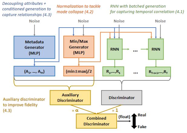
The first alteration has to do with the type of neural network used in the GAN. DoppelGANger, and other time series
GANs (Arnelid, Zec, & Mohammadiha, 2019; Mogren, 2016), rely on recurrent neural networks (RNNs) that are able
to capture temporal correlations. More specifically, DoppelGANger uses a popular type of RNN called long short-term
memory (LSTM). To illustrate the basic idea of RNN generators, say there is a univariate sequence of length τ . At
step i, the RNN will generate a value one step ahead, xi+1 , using information from previous values in the sequence
and the current state, {x1 , x2 , . . . , xi }. At each step the RNN keeps an encoded memory that summarizes relevant
information about the previous states, f ({x1 , x2 , . . . , xi−1 }; θ), allowing it to track temporal patterns (Goodfellow
et al., 2016). The RNN passes over the sequence τ times to produce the entire series. This idea can be extended
to multivariate time series. See Appendix A for more details on RNNs and LSTM. A common problem with RNN
generators is that long sequences require a very large number of passes of the RNN, which make it difficult to capture
longer-term correlations (Lin et al., 2020). To handle this problem, the creators of DoppelGANger use what they call
"batch generation". Instead of generating one step ahead in each pass, DoppelGANger generates S steps ahead, which
reduces the necessary number of passes. The authors of DoppelGANger suggest a value of S such that τ /S is around
50, but S can be tuned for specific tasks.
The next aspect of DoppelGANger is designed to mitigate mode collapse. The model uses a unique kind of normal-
ization for time series exhibiting a wide range of values across samples and series. For example, say in a given sample
one series has a range of 0 to 100, while another series in the sample has a range of -5 to 5. Rather than normalize by
the global minimum and maximum (-5 and 100) for all series, each series is normalized by its individual minimum and
maximum in that sample, and these values are stored as metadata for that series in the form min+max
2 . DoppelGANger
learns these metadata and generates a new minimum and maximum for rescaling each generated series. Experimenta-
tion indicates that this can help reduce mode collapse in many cases where ranges greatly vary between series (Lin et
al., 2020).
A useful feature of DoppelGANger is that it does not only generate synthetic time series, but also jointly generates
synthetic attributes (metadata) for those series. This is accomplished by using multiple generators. The first generates
metadata using a standard multilayer perceptron (MLP). These generated metadata are then given as inputs to another
MLP that generates the minimum and maximum metadata used for the normalization scheme described in the para-
graph above. Then all of the combined metadata are given as inputs to the LSTM that generates the synthetic time
series. To account for the different dimensionality and types of data being generated, there is an additional "auxiliary
discriminator", Daux , that measures loss on only the metadata. The Wasserstein loss of the two discriminators are
combined by the weighting scheme: minG maxD,Daux L(G, D) + αLaux (G, Daux ). A diagram of DoppelGANger’s
architecture can be seen in Figure 1.
3 Synthetic Data Generation
3.1 Data
Data were collected from the Federal Reserve Economic Data (FRED) website hosted by the Federal Reserve Bank of
St. Louis. Data were collected at a daily frequency for market yield on U.S. Treasuries at both a 1-year and 10-year
3Creating Disasters: Recession Forecasting with GAN-generated Synthetic Time Series Data
Figure 1: DoppelGANger’s Architecture
Source: "Using GANs for Sharing Networked Time Series Data: Challenges, Initial Promise, and
Open Questions" by Lin et al. URL: https://dl.acm.org/doi/pdf/10.1145/3419394.3423643
Copyright Information: Creative Commons Attribution 4.0 International Public License
17.5 1-year Treasury Yield
10-year Treasury Yield
15.0 Training Data Cutoff
12.5
10.0
Percent
7.5
5.0
2.5
0.0
1970 1980 1990 2000 2010 2020
Figure 2: U.S. Treasuries Yield Data
Note: Grey areas indicate recession
Sources: Board of Governors of the Federal Reserve System, Federal Reserve Bank of St. Louis,
NBER
constant maturity (Board of Governors of the Federal Reserve System (US), n.d.-a, n.d.-b). There are many possible
variations of short and long-term yield spread, but for this study, 1 and 10-year maturities were selected because they
have long histories available. An indicator for recession according to NBER was also collected at a daily frequency
(Federal Reserve Bank of St. Louis, n.d.). Note that yield data is only collected on weekdays. Figure 2 shows the
Treasury yield data. For the first task, DoppelGANger was trained on data ranging from 01-02-1962 to 12-30-2016.
The remaining data (from 01-03-2017 to 01-23-2023) was not used in training so that forecasting performance could
be evaluated on that time period.
3.2 Training
As with all deep learning models, DoppelGANger requires many samples to train on. So the training set was split
into samples of 125 day segments to be used as inputs to DoppelGANger. The features used in training were 1-year
Treasury Bill yield and 10-year Treasury Bond yield. For metadata, a single attribute was added to each sample
indicating whether or not a recession occurred at any point in that particular 125 day span.
A PyTorch implementation of DoppelGANger created by Gretel (Boyd, 2022) was used in training. Samples were
125 days in length and after some experimentation, S was set to 5; meaning there were 25 RNN passes over each
sample. The normalization scheme using the local minimum and maximum was applied to the yield data. In neural
network training, the learning rate is a hyperparameter that regulates the magnitude of updates at each step in the
4Creating Disasters: Recession Forecasting with GAN-generated Synthetic Time Series Data
Real Samples
4.0 9.0 5.8
3.8
8.5 5.6
Yield (Percent)
3.6 1-year Treasury Yield 8.0 5.4
10-year Treasury Yield
3.4
7.5
5.2
3.2
7.0
3.0 5.0
6.5
0 20 40 60 80 100 120 0 20 40 60 80 100 120 0 20 40 60 80 100 120
Days
Synthetic Samples
1.75 4.50
1.50 4.25 8.3
4.00 8.2
1.25
Yield (Percent)
3.75
1.00 Synthetic 1-year Treasury Yield 8.1
Synthetic 10-year Treasury Yield 3.50
0.75 8.0
3.25
0.50 7.9
3.00
0.25
2.75 7.8
0.00
0 20 40 60 80 100 120 0 20 40 60 80 100 120 0 20 40 60 80 100 120
Days
Figure 3: Comparison of real samples to synthetic samples
Note: The top row contains true data samples from the training set. The bottom row contains
generated data from DoppelGANger. The bottom right is an example of a generated yield curve
inversion.
Sources: Board of Governors of the Federal Reserve System, Federal Reserve Bank of St. Louis,
NBER, author
training process. Smaller learning rates are recommended for training and ensure that the gradient descent algorithm
does not take too large of steps and overshoot minimums (Glassner, 2021). The generator and discriminator learning
rates were both set equal to 10−4 , and training was run for 2000 epochs.
3.3 Evaluating generated data
After training the model, 1000 synthetic samples were generated. These are each 125 days in length and paired
with recession indicator metadata. Figure 3 shows three real samples from the training data and three synthetic
samples. Evaluating the data qualitatively, the synthetic samples appear quite similar to what one might expect from
the true data. The bottom right panel of Figure 3 is an example of a generated yield curve inversion, indicating that
DoppelGANger was able to learn from those unique cases as well as the standard cases where the 10-year yield should
be significantly higher than the 1-year yield. As far as metadata generation, approximately 18% of training samples
contained a positive indicator for recession. While approximately 17% of generated samples contained a positive
indicator for recession, meaning the samples containing recession data remained roughly proportional to the true data.
The key is that the trained generator now has the ability to produce as many fake recessions as needed.
In the training set, the correlation between 1-year and 10-year Treasury bond yields was 0.946. In the generated
samples, the correlation was 0.945. Figure 4 shows histograms for the 1-year and 10-year training data against their
synthetic counterparts. The synthetic data approximately follows the same distribution as the training data with a bit
more noise. In rare cases, the synthetic data may produce a negative yield or an outlier in terms of magnitude. These
are not ideal, but given that they are a negligible proportion of the generated samples, they likely do not have much
affect on downstream predictive tasks.
Given that the training data is split into segments, the model appears to struggle to capture the strength of the long-
term autocorrelations. For both 1-year and 10-year yields, the autocorrelation remains high even at a 100 day lag when
estimated on the full range of training data. It is difficult to assess autocorrelation for separated samples, however. The
5Creating Disasters: Recession Forecasting with GAN-generated Synthetic Time Series Data
Distribution of 1-year Yields Distribution of 10-year Yields
Real 0.16 Real
0.14
Synthetic 0.14 Synthetic
0.12
0.12
0.10
0.10
Density
Density
0.08
0.08
0.06 0.06
0.04 0.04
0.02 0.02
0.00 0.00
5 0 5 10 15 20 25 5 0 5 10 15 20 25
Yield Yield
Figure 4: Distributions of real and generated yields
Source: author’s calculations
1-year Yield Autocorrelations 10-year Yield Autocorrelations
1.0 1.0
0.8 0.8
0.6 0.6
Autocorrelation
Synthetic Synthetic
0.4 Real (training samples) 0.4 Real (training samples)
Real (full data) Real (full data)
0.2 0.2
0.0 0.0
0.2
0 20 40 60 80 100 0 20 40 60 80 100
lag (days) lag (days)
Figure 5: Estimated autocorrelations
Note: The synthetic and real (training samples) values are estimated as an average of autocorre-
lations across many samples. The real (full data) autocorrelation is estimated on the full range of
training data before being split into training samples.
Source: author’s calculations
method used was to assess the autocorrelation within each 125 day sample and average the autocorrelations across all
samples. This allows for comparison with the generated samples, which are independent 125 day segments.
When using this method, the training samples and generated samples show fairly similar patterns in their autocorre-
lations; however, they both show more rapid decline in autocorrelation than the estimates from the full training data.
You can see these patterns in Figure 5. So it appears that DoppelGANger was able to replicate the autocorrelations
from the training samples, but those samples underestimate the extent to which autocorrelation remains high in the
yield curve data. It should also be noted that higher lags have fewer data to estimate autocorrelation, and thus had
very high variance across samples. It is possible that lengthening the training samples to include more days could help
improve replication of long-term autocorrelations, but would come at the cost of fewer training samples. There is a
trade-off to consider between length of samples and quantity of samples when preparing training data. This should be
considered when deciding the horizon of forecasts that will be produced in downstream tasks.
The results shown in this section are an illustrative example of a successful training of DoppelGANger to Treasury data.
Not every training attempt was successful, however. Getting useful synthetic data required a bit of experimentation and
tuning, and even with the same training scheme, results can vary widely. In several training attempts, mode collapse
resulted in nearly all generated samples containing perfectly straight lines. DoppelGANger, like most GANs, can be
unstable and difficult to train but produces great results when properly trained.
4 Forecasting Treasury Yields
The first task is to evaluate forecasting performance of models trained on synthetic data against those trained on real
data. In order to do that, an LSTM model was trained to produce 1-day ahead forecasts of 1-year and 10-year Treasury
yields based on the previous 25 days of data.
6Creating Disasters: Recession Forecasting with GAN-generated Synthetic Time Series Data
Table 1: Forecasting performance for 1-day ahead forecasts over period January 3, 2017 to January 11, 2023.
Real Synthetic Combined
1-year Treasury RMSE 0.077 0.046 0.072
1-year Treasury MAPE 7.793 9.413 8.368
10-year Treasury RMSE 0.253 0.062 0.073
10-year Treasury MAPE 15.903 2.709 3.484
Table 2: Forecasting performance for 15-day ahead forecasts over period January 3, 2017 to January 11, 2023.
Real Synthetic Combined
1-year Treasury RMSE 0.244 0.355 0.307
1-year Treasury MAPE 77.736 84.610 58.448
10-year Treasury RMSE 0.425 0.543 0.269
10-year Treasury MAPE 25.075 30.503 13.557
Using actual data for 1-year and 10-year Treasury yields as shown in Figure 2, training samples were created by
splitting the data into a rolling window of 25 days. That is, the first 25 days of data make up the first sample, with
day 26 being its associated response. Then the window is moved forward by one day. Days 2-26 make up the second
sample, with an associated response from day 27, and so on. These samples were created over the time frame 01-02-
1962 to 12-30-2016, the same range of data that trained DoppelGANger. This produced 13,710 samples and associated
one-day ahead responses. We will refer to this set of samples as the real data training set.
As seen in section 3, DoppelGANger produced 1000 synthetic samples of yield data. These synthetic samples were
used to create forecast training data in the same fashion as the real data training set described above. A rolling 25 day
window split up training samples and responses within each synthetic sample. Each 125 day segment of synthetic data
was able to generate 100 training samples and responses for a total of 100,000 synthetic training samples. We will
refer to this as the synthetic data training set.
Finally, a training set was created by combining the real data training set and the synthetic data training set. The idea
is that the LSTM model will be trained on real data that is augmented by synthetic data in order to allow for more
samples. This training set has 113,710 samples and will be referred to as the combined data training set.
The model trained for forecasting is a deep neural network with two stacked LSTM layers, each with a hyperbolic
tangent (tanh) activation function, followed by a dropout layer and a dense layer with 2 nodes for the 2 features (1-
year and 10-year Treasury yield). A diagram of this model can be seen in Figure C.1. The model used a mean-squared
error loss function and Adam optimizer (Kingma & Ba, 2014). This model was trained with each of the three training
sets - real, synthetic, and combined - each for 50 epochs. Each trained model then produced one-day ahead forecasts
for a test set containing real Treasury yield data from 01-03-2017 to 01-11-2023. Forecasting performance over this
test set, measured by root mean square error (RMSE) and mean absolute percentage error (MAPE), can be seen in
Table 1.
The LSTM model trained on synthetic data outperformed the other models in every metric except for the MAPE for
1-year Treasury yield. Interestingly, the model trained on combined data performed much better than the model trained
on real data for the 10-year Treasury yield, but still did not match the performance of the model trained on synthetic
data only. These results imply that models trained on synthetic data can improve forecasting performance over a model
trained on only real data, likely due to the increased availability of training data.
The same LSTM model architecture was then used again to test the forecasting performance of longer-range forecasts.
This time, rather than providing responses of a single day ahead, the response was a vector of 15 days beyond the
end of the training sample. The LSTM was thus trained to take a sample of 25 days and predict yield values for the
following 15 days. Again, three models were trained on real data, synthetic data, and combined real and synthetic
data. Forecasting performance was evaluated for the 15th day of the generated predictions, and these metrics can be
found in Table 2.
7Creating Disasters: Recession Forecasting with GAN-generated Synthetic Time Series Data
1-Year Treasury Yield Forecasts: 1-Day Ahead
5 5 5
Actual Actual Actual
Forecast - Real Data Forecast - Synthetic Data Forecast - Combined Data
4 4 4
Yield (Percent)
3 3 3
2 2 2
1 1 1
0 0 0
2017 2018 2019 2020 2021 2022 2023 2017 2018 2019 2020 2021 2022 2023 2017 2018 2019 2020 2021 2022 2023
4.5
10-Year Treasury Yield Forecasts: 1-Day Ahead
4.5 4.5
Actual Actual Actual
4.0 Forecast - Real Data 4.0 Forecast - Synthetic Data 4.0 Forecast - Combined Data
3.5 3.5 3.5
3.0
Yield (Percent)
3.0 3.0
2.5 2.5 2.5
2.0 2.0 2.0
1.5 1.5 1.5
1.0 1.0 1.0
0.5 0.5 0.5
2017 2018 2019 2020 2021 2022 2023 2017 2018 2019 2020 2021 2022 2023 2017 2018 2019 2020 2021 2022 2023
Figure 6: 1-day ahead forecasts for each type of training data
Sources: Board of Governors of the Federal Reserve System, Federal Reserve Bank of St. Louis,
NBER, author
1-Year Treasury Yield Forecasts: 15-Day Ahead
5 5
5 Actual Actual Actual
Forecast - Real Data Forecast - Synthetic Data Forecast - Combined Data
4 4
4
Yield (Percent)
3 3
3
2 2 2
1 1 1
0 0 0
2017 2018 2019 2020 2021 2022 2023 2017 2018 2019 2020 2021 2022 2023 2017 2018 2019 2020 2021 2022 2023
10-Year Treasury Yield Forecasts: 15-Day Ahead
4.5
4.5 Actual 6 Actual Actual
4.0 Forecast - Real Data Forecast - Synthetic Data 4.0 Forecast - Combined Data
3.5 5 3.5
Yield (Percent)
3.0 4 3.0
2.5 2.5
3 2.0
2.0
1.5 2 1.5
1.0 1 1.0
0.5 0.5
2017 2018 2019 2020 2021 2022 2023 2017 2018 2019 2020 2021 2022 2023 2017 2018 2019 2020 2021 2022 2023
Figure 7: 15-day ahead forecasts for each type of training data
Sources: Board of Governors of the Federal Reserve System, Federal Reserve Bank of St. Louis,
NBER, author
8Creating Disasters: Recession Forecasting with GAN-generated Synthetic Time Series Data
The longer-range forecasting model trained on only synthetic data consistently had the worst performance. This is not
surprising, as it was shown in section 3 that the synthetic data struggled to capture the longer-range autocorrelation of
the true data. In longer-range forecasting, the model trained on combined real and synthetic data fared the best. This
could potentially be due to the fact that the combined data model benefits from both learning the true structure of the
real data and an increased availability of training samples from the synthetic data. Overall, it appears there is a benefit
to using synthetic data in forecasting Treasury yields.
5 Predicting Recessions
The second task of this study is to test if using synthetic data can improve the prediction of an upcoming recession.
The framework for predicting an upcoming recession is to train a classification model to provide a probability that a
recession will occur any time in the next 250 days. The challenge for these models is that when using available historic
data, there are very few actual recessions for training and testing. In the range of dates for which Treasury yield data
is available, there are only 8 recessions that have occurred. One of those recessions (2020) is a result of COVID-19,
and could not possibly be predicted by economic factors. That leaves 7 recessions to train and test a model; however,
with synthetic data, we are able to produce as many fake recessions as needed.
5.1 Generating data
In order to build classification models to predict upcoming recessions, new synthetic data must be generated. The
primary changes in this round of synthetic data generation is that a new attribute (metadata) was added to indicate a
future recession and DoppelGANger was trained on a smaller set of data. The samples are also only 30 days long,
rather than the 125 day samples created before.
For this task, DoppelGANger was trained on the time period 01-02-1962 to 12-31-1984. This time period contains 4
recessions, which leaves 3 recessions for testing downstream predictive performance, as seen in Figure B.1. In addition
to the indicator for a recession used in the previous training of DoppelGANger, an indicator for a future recession was
added. This future recession indicator takes value 1 for samples in which a recession occurred any time in the 250 days
following the sample, and 0 otherwise. In other words, this indicator labels each sample by whether or not it precedes
a recession by at most 250 days. The features are still 1-year and 10-year Treasury yields, while the metadata now has
two dimensions - recession indicator and future recession indicator.
The generated samples from this version of DoppelGANger performed equally well in terms of fidelity metrics as the
generated samples displayed in section 3. This iteration of DoppelGANger was also able to capture the correlation
between features and the overall distributions of both 1-year and 10-year Treasury yields, but similarly struggled to
capture the autocorrelation structure. Full metrics can be found in Appendix B.
5.2 Classification models
To test if synthetic data can improve a model’s ability to predict future recessions, two models were used - logistic
regression and an LSTM classifier. The goal is to give these models the previous 30 days of 1-year and 10-year
Treasury data as an input and produce a predicted probability that a recession will occur at some point in the following
250 days. Each sample of 30 days in the training data is paired with an indicator for whether or not a recession occurred
in the 250 days following that sample, including the synthetic data which generated that future recession indicator as
metadata.
The logistic regression specification was treated like an autoregressive model in that each day in the 30 day sample
was input as its own feature. In other words, each training sample had 60 features - 1-year and 10-year Treasury yields
for the most recent day and 29 lags for each variable. In order to control for a large amount of features, the models
were fit with an L1 regularization. This means that there was a penalty on the estimated coefficients which shrinks
them toward zero and performs an automated form of feature selection to reduce the dimensionality of the model. The
optimization problem for logistic regression under L1 regularization is (Lee, Lee, Abbeel, & Ng, 2006):
M
X
min −log p(y (i) |x(i) ; β) + λ||β||1
β
i=1
Where β are the estimated coefficients and λ is a hyperparameter that controls the amount of regularization. The
logistic regression uses a gradient descent algorithm to minimize the negative log-likelihood of the model with the
added constraint that the L1 norm of the model be kept reasonably small.
9Creating Disasters: Recession Forecasting with GAN-generated Synthetic Time Series Data
The second model used was an LSTM-based classification model. It works in much the same way as the LSTM
models used in the forecasting task of section 4, with the exception that it produces probabilities of recession rather
than forecasting. The architecture of the LSTM classification model contained a single LSTM layer with a hyperbolic
tangent activation function followed by a dropout layer, then a dense layer with 100 nodes and a hyperbolic tangent
activation function. Finally, there was a dense layer with 2 nodes and a softmax activation to ensure that the model
produced probabilities. This model was trained with a categorical cross-entropy loss function and an Adam optimizer
for 50 epochs. A diagram of this model can be found in Figure C.2.
Both the logistic regression and LSTM-based classifier were trained on samples of real data, synthetic data, and a
combination of real and synthetic data. The real data comprised 30 day rolling window samples from 01-02-1962 to
12-31-1984, the same range of dates that trained DoppelGANger to produce synthetic data for the classification task.
Thus, there were 5,701 real training samples. The synthetic training data comprised 50,000 30-day samples produced
by DoppelGANger and their associated future recession indicator. The combined training data simply combined both
the real and synthetic training samples into one training set.
The output of each model is a probability of recession in the next 250 days based on the previous 30 days of 1-year
and 10-year Treasury yield data.
5.3 Evaluating Recession Predictions
The test set to evaluate each model’s ability to predict future recessions covered the time period 01-02-1985 to 06-30-
2009. This time period contains 3 recessions, and thus provides the opportunity to see how strong of a signal each
model produces leading up to a new set of recessions. This section attempts to evaluate the performance of each model
at assigning high probabilities of recession in the days leading up to a recession and low probabilities when a recession
is not imminent.
It should be noted that performance in this setting is quite difficult to evaluate due to the somewhat subjective nature of
the classification labels. It is somewhat arbitrary to say a recession signal is only good if it appears within 250 days of
the recession. So while strong recession signals more than 250 days out are considered false positives for this paper’s
purposes, others may argue those are valid early signals. The other aspect to consider is that policy actions are often
taken to prevent recessions that are not considered by these models. So while a high probability of recession may seem
like a false positive, it is possible that the model was signaling a recession that may have occurred in the absence of
policy action. With these caveats in mind, we will attempt to evaluate each model as objectively as possible.
5.3.1 Logistic Regression Performance
The probability of recession predictions produced by each logistic regression model can be found in Figure 8. The
model trained on only real data gives very weak signals, never producing a probability above 30 percent. The model
trained on synthetic data follows much the same pattern as that of the model trained on real data, but produces much
stronger signals, often reaching probabilities above 80 percent. The downside is that this model is much noisier.
This is not surprising, as the synthetic data inherently contains more noise than the real data. The model trained on the
combined data is similar to the model trained on synthetic data, though with a slightly weaker signal. It should be noted
that the models that trained on additional synthetic recessions were better able to recognize upcoming recessions, but
were also more sensitive to false positives. This can be seen in the period preceding the 2001 recession. The models
trained with synthetic data gave very strong recessionary signals in 1996 and again in 1998-1999.
The ROC curves (a graph that plots the true positive rate against the false positive rate) for each logistic regression
model can be seen in Figure 10. A useful summary of classification performance is the area under the ROC curve
(AUC). The higher the AUC, the better the predictive performance. In the case of logistic regression, the ROC curves
are very similar. The model trained on real data has a slight edge over the other two. This follows intuitively from the
fact that all three models tend to give the same signal, albeit at very different levels. Rescaling the real data model such
that a 25 percent probability of recession is considered a strong indicator of an upcoming recession puts it in line with
the other models, with the added benefit of less noise. So while synthetic data does not appear to improve performance
for the logistic regression, it at least produces estimates that are comparable to a model trained on real data - a good
sign that DoppelGANger has produced high-fidelity synthetic data.
5.3.2 LSTM Classifier Performance
The probability of recession predictions produced by each LSTM classifier model can be found in Figure 9. Here,
the benefits of synthetic data are much more clear. The model trained on only real data gives short-lived spikes in
probability and produces strong false positives in the mid to late 1990s. It also gives no signal at all of the 2008
10Creating Disasters: Recession Forecasting with GAN-generated Synthetic Time Series Data
1.0
Probability of Recession from Logistic Regression
Prob. of Recession (Synthetic Data)
Prob. of Recession (Combined Data)
Prob. of Recession (Real Data)
0.8
Probability of Recession
0.6
0.4
0.2
0.0
1984 1988 1992 1996 2000 2004 2008
Figure 8: Probability of Recession as predicted by logistic regression
Note: Grey areas indicate recession. Black dashed lines indicate 250 days prior to the start of the
next recession.
Source: NBER, author’s calculations
recession. The model trained on synthetic data provides more prolonged signals of recession and produces weaker
false positive signals in the mid to late 1990s. Again, the synthetic data produces much noisier estimates. The model
trained on the combined data largely follows the same patterns of the model trained on synthetic data with somewhat
less noise. Both the synthetic data and combined data models provide weak signals leading up to the 2008 recession.
The LSTM models trained with synthetic data appear to perform quite well at providing high probabilities just prior
to recessions while not being overly sensitive to minor yield curve inversions. The LSTM models overall did a worse
job of predicting the 2008 recession relative to the logistic regression models, but within the class of LSTM models,
synthetic data clearly improved the ability to predict the 2008 recession.
The ROC curves for the LSTM models can also be found in Figure 10. Here the AUC is clearly much higher for the
model trained on synthetic data (0.86) and the model trained on combined data (0.81) than the AUC for the model
trained only on real data (0.69). It appears that allowing the LSTM models to train on additional fake recessions does
produce a significant improvement in predictive ability.
6 Conclusion
GANs have shown great promise in generating synthetic data for a wide range of tasks. This paper serves as a proof of
concept, showing that GAN-generated synthetic time series data can be useful in forecasting applications, particularly
in economic settings. For US financial and economic data, there is only one history. Previously, economic forecasters
had access only to the information provided by the limited recessions that have occurred and the single history of
Treasury yields. With GANs, and particularly DoppelGANger, researchers and forecasters can now produce as many
synthetic histories as they please. Models can be trained on a much larger number of recessions and learn from a much
wider range of samples.
This paper shows that although these synthetic recessions are merely replicating the conditions of the true recessions
they were trained on, they can actually provide information above and beyond the true recessions when performing
downstream predictive tasks.
The models used in this paper for economic forecasting and recession prediction are fairly simple models that rely only
on 1-year and 10-year Treasury yields. They are not fine-tuned or conditioned on other economic variables. They are
merely illustrations of the comparative performance of simple models trained with real and synthetic data. This means
that predictive performance could likely be vastly improved in future work by applying the synthetic data framework
of this paper to more advanced econometric techniques, though that remains to be seen. Also note that despite the
11Creating Disasters: Recession Forecasting with GAN-generated Synthetic Time Series Data
1.0
Probability of Recession from LSTM
Prob. of Recession (Synthetic Data)
Prob. of Recession (Combined Data)
Prob. of Recession (Real Data)
0.8
Probability of Recession
0.6
0.4
0.2
0.0
1984 1988 1992 1996 2000 2004 2008
Figure 9: Probability of Recession as predicted by LSTM model
Note: Grey areas indicate recession. Black dashed lines indicate 250 days prior to the start of the
next recession.
Source: NBER, author’s calculations
ROC Curves for Logistic Regression Models ROC Curves for LSTM Models
1.0 1.0
0.8 0.8
True Positive Rate
True Positive Rate
0.6 0.6
0.4 0.4
0.2 Logistic Regression (Real), AUC= 0.9089 0.2 LSTM (Real), AUC= 0.6871
Logistic Regression (Synthetic), AUC= 0.8983 LSTM (Synthetic), AUC= 0.8559
0.0 Logistic Regression (Combined), AUC= 0.9056 0.0 LSTM (Combined), AUC= 0.8114
0.0 0.2 0.4 0.6 0.8 1.0 0.0 0.2 0.4 0.6 0.8 1.0
False Positive Rate False Positive Rate
Figure 10: ROC curves for all probability of recession models
Source: author’s calculations
difficulty in capturing long-term autocorrelations for Treasury yield data, many of the models trained with synthetic
data were still able to show improvements over models trained with only real data. Further improving the fidelity of
the synthetic data could potentially produce even greater improvements.
In future work, this framework could be extended to a wide range of applications in which rare events need to be
predicted - such as rare atmospheric events or the occurrence of disease - provided that high-fidelity synthetic data
can be produced. This is certainly not the first paper to use synthetic data to improve predictive models, but it shows
another useful application of the technique. As GANs and other machine learning techniques advance at a rapid pace,
there is great potential for further exploration of how high-fidelity synthetic data can improve time series forecasting.
12Creating Disasters: Recession Forecasting with GAN-generated Synthetic Time Series Data
Appendices
A RNNs and LSTM
This appendix is adapted from Chapter 10 of Goodfellow et al. (2016).
Recurrent neural networks (RNNs) are a form of neural network designed to capture information from sequence data.
The input data to RNNs are read sequentially, with information about previous inputs being stored as the RNN works
its way through the sequence. The current state, h(t) , is a function of all previous states processed before step t and
current features, x(t) .
h(t) = f (h(t−1) , x(t) ; θ)
Where θ represents the parameters (weights) that the learning algorithm attempts to optimize. At each time step, the
current state summarizes useful information from the current input, as well as all previous inputs, and then uses that
summary as an input to the next time step. The advantage of using recurrence in this way is that the model can learn
temporal patterns in the sequence of inputs. Using the same f and θ at each time step simplifies the training process
to learning a single model for all time steps. An unrolled graph displaying an example RNN can be found in Figure
A.1.
Figure A.1: An example of an unfolded RNN graph
Source: Author, based on Figure 10.3 of (Goodfellow et al., 2016)
Note: U , V, W represent weights between layers. Not shown are activation functions that will
accompany these weights.
In Figure A.1, h(i) represents hidden states that are used as an input to the next time step, x(i) represents the features
input at each time step, and o(i) represents the outputs of each time step. W represents the weights that parameterize
connections between hidden layers, U represents weights between input layers and hidden layers, and V represents
weights between hidden layers and output layers. o(t) will be compared to the target y (t) when computing the loss
function for backpropagation. There are many different configurations of RNNS, and this chart represents one of the
most simple configurations.
Long-term interactions present in sequences can be hard to estimate with a standard RNN. As the gradients are back-
propagated through a large number of time steps, they tend to become smaller and smaller until they vanish. It is also
possible to create exploding gradients from exponential growth. In the more common case of vanishing gradients,
time steps further back in the sequence will have very small gradients, thus making it difficult to learn long-term
interactions.
A popular way of dealing with the vanishing gradient problem is by using a gated RNN such as "long short-term
memory" (LSTM) networks. The name long short-term memory refers to the fact that these networks capture the
short-term changes in state from one step to the next (short-term memory), but also sometimes choose to keep past
information for many steps (long-term memory) (Glassner, 2021). LSTM networks replace the hidden layers of the
common RNN with LSTM "cells". These cells are composed of multiple networks. A network known as the "forget
gate" controls how much past information to discard by moving weights on previous units toward zero. Another
network known as "input gate" controls whether inputs should be accumulated into the current state. Finally, an
"output gate" controls the cell’s output. An LSTM cell can be seen in Figure A.2
The diagram of an LSTM cell displays the basic function of gates within the LSTM cell. The inputs (x(t) and h(t−1) )
are provided to the input unit and each of the three gates. All of the gates use a sigmoid activation function. The
13Creating Disasters: Recession Forecasting with GAN-generated Synthetic Time Series Data
Figure A.2: A single LSTM cell. Cells replace the traditional hidden units of an RNN.
Source: Author, based on Figure 10.16 of (Goodfellow et al., 2016)
Note: Gates use a sigmoid activation function.
input gate can "shut off" the input through a sigmoid function and thus determines what inputs to store in the current
state. The state has a recurrent connection to itself (a self-loop) whose effect is controlled by the output of the forget
gate. This effectively decides when it is appropriate to "forget" prior information. The output also has a gate with a
sigmoid activation. Each gate is a network with its own input and recurrent weights to train. All of these gates allow
for the LSTM network to dynamically control the amount of long-term memory that is relevant. Most importantly,
this framework allows the gradients to backpropagate for long durations without vanishing or exploding.
B Synthetic Data fidelity metrics for classification models
The figures below display the fidelity metrics for the synthetic data generated for the recession classifier task. The
correlation between 1-year and 10-year Treasury yields in the training samples was 0.950. The same correlation in the
synthetic samples was 0.953.
17.5 1-year Treasury Yield
10-year Treasury Yield
Training Data Cutoff
15.0
12.5
10.0
Percent
7.5
5.0
2.5
0.0
1970 1980 1990 2000 2010 2020
Figure B.1: U.S. Treasuries Yield Data
Note: Grey areas indicate recession. The training sample contained 4 recessions, leaving 3 reces-
sions for testing the classification models (the 2020 recession is excluded from the test set).
Sources: Board of Governors of the Federal Reserve System, Federal Reserve Bank of St. Louis,
NBER
14Creating Disasters: Recession Forecasting with GAN-generated Synthetic Time Series Data
Real Samples
6.2 4.0
4.0
6.1
3.8 3.8
6.0
Yield (Percent)
3.6 1-year Treasury Yield 5.9 3.6
10-year Treasury Yield 5.8
3.4
5.7 3.4
3.2 5.6
3.2
3.0 5.5
0 5 10 15 20 25 30 0 5 10 15 20 25 30 0 5 10 15 20 25 30
Days
Synthetic Samples
5.4
11.50
7.2
11.25 5.2
7.1
Yield (Percent)
11.00
Synthetic 1-year Treasury Yield 5.0
10.75 Synthetic 10-year Treasury Yield 7.0
10.50 4.8
6.9
10.25 4.6
10.00 6.8
4.4
0 5 10 15 20 25 30 0 5 10 15 20 25 30 0 5 10 15 20 25 30
Days
Figure B.2: Comparison of real samples to synthetic samples for classifier
Note: The top row contains true data samples from the training set. The bottom row contains
generated data from DoppelGANger.
Sources: Board of Governors of the Federal Reserve System, Federal Reserve Bank of St. Louis,
NBER, author
0.16
Distribution of 1-year Yields Distribution of 10-year Yields
0.200
Real Real
0.14 Synthetic 0.175 Synthetic
0.12 0.150
0.10 0.125
Density
Density
0.08 0.100
0.06 0.075
0.04 0.050
0.02 0.025
0.00 0.000
5 0 5 10 15 20 25 5 0 5 10 15 20 25
Yield Yield
Figure B.3: Distributions of real and generated yields for classifier
Source: author’s calculations
15Creating Disasters: Recession Forecasting with GAN-generated Synthetic Time Series Data
1-year Yield Autocorrelations 10-year Yield Autocorrelations
1.0 1.0
0.8 0.8
0.6 0.6
Autocorrelation
Synthetic Synthetic
0.4 Real (training samples) 0.4 Real (training samples)
Real (full data) Real (full data)
0.2 0.2
0.0 0.0
0.2 0.2
0 5 10 15 20 25 30 0 5 10 15 20 25 30
lag (days) lag (days)
Figure B.4: Estimated autocorrelations for classifier
Note: The synthetic and real (training samples) values are estimated as an average of autocorre-
lations across many samples. The real (full data) autocorrelation is estimated on the full range of
training data before being split into training samples.
Source: author’s calculations
16Creating Disasters: Recession Forecasting with GAN-generated Synthetic Time Series Data
C LSTM Model Diagrams
Figure C.1: Diagram of network used for forecasting task
Note: This diagram represents the LSTM model used for 1-day ahead forecasts. For 15-day ahead
forecasts, the model was altered to allow for an output of shape 15x2.
Source: Author
Figure C.2: Diagram of network used for classification task
Source: Author
17Creating Disasters: Recession Forecasting with GAN-generated Synthetic Time Series Data
References
Arnelid, H., Zec, E. L., & Mohammadiha, N. (2019). Recurrent conditional generative adversarial networks for
autonomous driving sensor modelling. In 2019 ieee intelligent transportation systems conference (itsc) (p. 1613-
1618). doi: doi:10.1109/ITSC.2019.8916999
Bernard, H., & Gerlach, S. (1998). Does the term structure predict recessions? the international evidence. International
Journal of Finance and Economics.
Board of Governors of the Federal Reserve System (US). (n.d.-a). Market yield on u.s. treasury securities at 10-year
constant maturity, quoted on an investment basis [dgs10]. retrieved from FRED, Federal Reserve Bank of St.
Louis. Retrieved from https://fred.stlouisfed.org/series/DGS10 (Date accessed: January 12, 2023)
Board of Governors of the Federal Reserve System (US). (n.d.-b). Market yield on u.s. treasury securities at 1-year
constant maturity, quoted on an investment basis [dgs1]. retrieved from FRED, Federal Reserve Bank of St.
Louis. Retrieved from https://fred.stlouisfed.org/series/DGS1 (Date accessed: January 12, 2023)
Boyd, K. (2022). Create synthetic time-series data with doppelganger and pytorch. Retrieved from https://
gretel.ai/blog/create-synthetic-time-series-with-doppelganger-and-pytorch
Business cycle dating. (2023). Retrieved from https://www.nber.org/research/business-cycle-dating
Estrella, A., & Hardouvelis, G. (1991). The term structure as a predictor of real economic activity. Journal of Finance.
Estrella, A., & Mishkin, F. S. (1996). The yield curve as a predictor of u.s. recessions. Current Issues in Economics
and Finance.
Fawaz, H. I., Forestier, G., Weber, J., Idoumghar, L., & Muller, P.-A. (2018). Data augmentation using synthetic data
for time series classification with deep residual networks. arXiv. Retrieved from https://arxiv.org/abs/
1808.02455 doi: doi:10.48550/ARXIV.1808.02455
Federal Reserve Bank of St. Louis. (n.d.). Nber based recession indicators for the united states from the period
following the peak through the trough [usrecd]. retrieved from FRED, Federal Reserve Bank of St. Louis.
Retrieved from https://fred.stlouisfed.org/series/USRECD (Date accessed: January 12, 2023)
Frid-Adar, M., Klang, E., Amitai, M., Goldberger, J., & Greenspan, H. (2018). Synthetic data augmentation using gan
for improved liver lesion classification. In 2018 ieee 15th international symposium on biomedical imaging (isbi
2018) (p. 289-293). doi: doi:10.1109/ISBI.2018.8363576
Glassner, A. (2021). Deep learning: A visual approach. No Starch Press.
Goodfellow, I., Bengio, Y., & Courville, A. (2016). Deep learning. MIT Press. (http://www.deeplearningbook
.org)
Goodfellow, I., Pouget-Abadie, J., Mirza, M., Xu, B., Warde-Farley, D., Ozair, S., . . . Bengio, Y. (2014). Gener-
ative adversarial nets. In Z. Ghahramani, M. Welling, C. Cortes, N. Lawrence, & K. Weinberger (Eds.), Ad-
vances in neural information processing systems (Vol. 27). Curran Associates, Inc. Retrieved from https://
proceedings.neurips.cc/paper/2014/file/5ca3e9b122f61f8f06494c97b1afccf3-Paper.pdf
Karras, T., Laine, S., & Aila, T. (2018). A style-based generator architecture for generative adversarial networks.
arXiv. Retrieved from https://arxiv.org/abs/1812.04948 doi: doi:10.48550/ARXIV.1812.04948
Kessel, R. A. (1965). The cyclical behavior of the term structure of interest rates. National Bureau of Economic
Research Occasional Paper No. 91.
Kingma, D. P., & Ba, J. (2014). Adam: A method for stochastic optimization. arXiv. Retrieved from https://
arxiv.org/abs/1412.6980 doi: doi:10.48550/ARXIV.1412.6980
Lee, S.-I., Lee, H., Abbeel, P., & Ng, A. (2006, 01). Efficient l1 regularized logistic regression. In (Vol. 21).
Lin, Z., Jain, A., Wang, C., Fanti, G., & Sekar, V. (2020, October). Using GANs for sharing networked time series
data. In Proceedings of the ACM internet measurement conference. ACM. Retrieved from https://doi.org/
10.1145/3419394.3423643 doi: doi:10.1145/3419394.3423643
Mogren, O. (2016). C-rnn-gan: Continuous recurrent neural networks with adversarial training. arXiv. Retrieved
from https://arxiv.org/abs/1611.09904 doi: doi:10.48550/ARXIV.1611.09904
Nikolenko, S. I. (2019). Synthetic data for deep learning. arXiv. Retrieved from https://arxiv.org/abs/
1909.11512 doi: doi:10.48550/ARXIV.1909.11512
Zhu, J.-Y., Park, T., Isola, P., & Efros, A. A. (2017). Unpaired image-to-image translation using cycle-
consistent adversarial networks. arXiv. Retrieved from https://arxiv.org/abs/1703.10593 doi:
doi:10.48550/ARXIV.1703.10593
18You can also read