CONTINUAL NORMALIZATION: RETHINKING BATCH NORMALIZATION FOR ONLINE CONTINUAL LEARNING
←
→
Page content transcription
If your browser does not render page correctly, please read the page content below
Published as a conference paper at ICLR 2022

C ONTINUAL N ORMALIZATION :
R ETHINKING BATCH N ORMALIZATION                                              FOR       O NLINE
C ONTINUAL L EARNING
 Quang Pham1 , Chenghao Liu2 , Steven C.H. Hoi 1,2
 1
   Singapore Management University
 hqpham.2017@smu.edu.sg
 2
   Salesforce Research Asia
 {chenghao.liu, shoi}@salesforce.com

                                            A BSTRACT
         Existing continual learning methods use Batch Normalization (BN) to facilitate
         training and improve generalization across tasks. However, the non-i.i.d and non-
         stationary nature of continual learning data, especially in the online setting, am-
         plify the discrepancy between training and testing in BN and hinder the perfor-
         mance of older tasks. In this work, we study the cross-task normalization effect of
         BN in online continual learning where BN normalizes the testing data using mo-
         ments biased towards the current task, resulting in higher catastrophic forgetting.
         This limitation motivates us to propose a simple yet effective method that we call
         Continual Normalization (CN) to facilitate training similar to BN while mitigat-
         ing its negative effect. Extensive experiments on different continual learning algo-
         rithms and online scenarios show that CN is a direct replacement for BN and can
         provide substantial performance improvements. Our implementation is available
         at https://github.com/phquang/Continual-Normalization.

1    I NTRODUCTION
Continual learning (Ring, 1997) is a promising approach towards building learning systems with
human-like capabilities. Unlike traditional learning paradigms, continual learning methods observe
a stream of tasks and simultaneously perform well on all tasks with limited access to previous
data. Therefore, they have to achieve a good trade-off between retaining old knowledge (French,
1999) and acquiring new skills, which is referred to as the stability-plasticity dilemma (Abraham
& Robins, 2005). Continual learning has been a challenging research problem, especially for deep
neural networks because of their ubiquity and promising results on many applications (LeCun et al.,
2015; Parisi et al., 2019).
While most previous works focus on developing strategies to alleviate catastrophic forgetting and
facilitating knowledge transfer (Parisi et al., 2019), scant attention has been paid to the backbone
they used. In standard backbone networks such as ResNets (He et al., 2016), it is natural to use Batch
Normalization (BN) (Ioffe & Szegedy, 2015), which has enabled the deep learning community to
make substantial progress in many applications (Huang et al., 2020). Although recent efforts have
shown promising results in training deep networks without BN in a single task learning (Brock
et al., 2021), we argue that BN has a huge impact on continual learning. Particularly, when using
an episodic memory, BN improves knowledge sharing across tasks by allowing data of previous
tasks to contribute to the normalization of current samples and vice versa. Unfortunately, in this
work, we have explored a negative effect of BN that hinders its performance on older tasks and
thus increases catastrophic forgetting. Explicitly, unlike the standard classification problems, data in
continual learning arrived sequentially, which are not independent and identically distributed (non-
i.i.d). Moreover, especially in the online setting (Lopez-Paz & Ranzato, 2017), the data distribution
changes over time, which is also highly non-stationary. Together, such properties make the BN’s
running statistics heavily biased towards the current task. Consequently, during inference, the model
normalizes previous tasks’ data using the moments of the current task, which we refer to as the
“cross-task normalization effect”.

                                                   1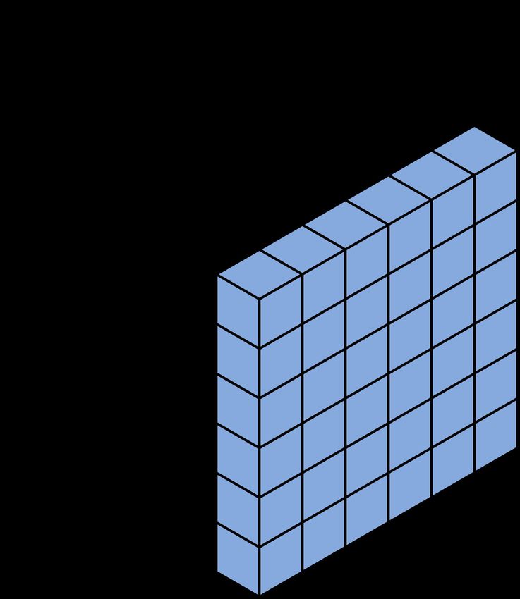
Published as a conference paper at ICLR 2022
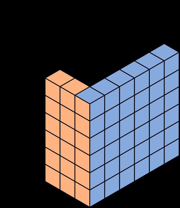
Batch Norm Instance Norm Group Norm Continual Norm
H, W
H, W
H, W
H, W
C N C N C N C N
Figure 1: An illustration of different normalization methods using cube diagrams derived from Wu
& He (2018). Each cube represents a feature map tensor with N as the batch axis, C as the channel
axis, and (H,W) as the channel axes. Pixels in blue are normalized by the same moments calculated
from different samples while pixels in orange are normalized by the same moments calculated from
within sample. Best viewed in colors.
Although using an episodic memory can alleviate cross-task normalization in BN, it is not possi-
ble to fully mitigate this effect without storing all past data, which is against the continual learning
purposes. On the other hand, spatial normalization layers such as GN (Wu & He, 2018) do not
perform cross-task normalization because they normalize each feature individually along the spatial
dimensions. As we will empirically verify in Section 5.1, although such layers suffer less forget-
ting than BN, they do not learn individual tasks as well as BN because they lack the knowledge
transfer mechanism via normalizing along the mini-batch dimension. This result suggests that a
continual learning normalization layer should balance normalizing along the mini-batch and spatial
dimensions to achieve a good trade-off between knowledge transfer and alleviating forgetting. Such
properties are crucial for continual learning, especially in the online setting (Lopez-Paz et al., 2017;
Riemer et al., 2019), but not satisfied by existing normalization layers. Consequently, we propose
Continual Normalization (CN), a novel normalization layer that takes into account the spatial infor-
mation when normalizing along the mini-batch dimension. Therefore, our CN enjoys the benefits
of BN while alleviating the cross-task normalization effect. Lastly, our study is orthogonal to the
continual learning literature, and the proposed CN can be easily integrated into any existing methods
to improve their performances across different online protocols.
In summary, we make the following contributions. First, we study the benefits of BN and its cross-
task normalization effect in continual learning. Then, we identify the desiderata of a normalization
layer for continual learning and propose CN, a novel normalization layer that improves the perfor-
mance of existing continual learning methods. Lastly, we conduct extensive experiments to validate
the benefits and drawbacks of BN, as well as the improvements of CN over BN.
2 N OTATIONS AND P RELIMINARIES
This section provides the necessary background of continual learning and normalization layers.
2.1 N OTATIONS
We focus on the image recognition problem and denote an image as x ∈ RW ×H×C , where W , H,
C are the image width, height, and the number of channels respectively. A convolutional neural
network (CNN) with parameter θ is denoted as fθ (·). A feature map of a mini-batch B is defined
as a ∈ RB×C×W ×H . Finally. each image x is associated with a label y ∈ {1, 2 . . . , Y } and a task
identifier t ∈ {1, 2, . . . , T }, that is optionally revealed to the model, depending on the protocol.
2.2 C ONTINUAL L EARNING
Continual learning aims at developing models that learn continuously over a stream of tasks. In
literature, extensive efforts have been devoted to develop better continual learning algorithms, rang-
ing from the dynamic architectures (Rusu et al., 2016; Serra et al., 2018; von Oswald et al., 2020;
Yoon et al., 2018; Li et al., 2019; Xu & Zhu, 2018), experience replay (Lin, 1992; Chaudhry et al.,
2019b; Aljundi et al., 2019a; Riemer et al., 2019; Rolnick et al., 2019; Wu et al., 2019), regulariza-
tion (Kirkpatrick et al., 2017; Zenke et al., 2017; Aljundi et al., 2018; Ritter et al., 2018), to fast and
slow frameworks (Pham et al., 2020; 2021). Our work takes an orthogonal approach by studying the
benefits and drawbacks of BN, which is commonly used in most continual learning methods.
2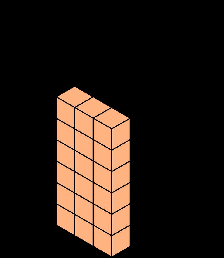
Published as a conference paper at ICLR 2022

Continual Learning Protocol We focus on the online continual learning protocol (Lopez-Paz &
Ranzato, 2017) over T tasks. At each step, the model only observes training samples drawn from
the current training task data and has to perform well on the testing data of all observed tasks so far.
Moreover, data comes strictly in a streaming manner, resulting in a single epoch training setting.
Throughout this work, we conduct experiments on different continual learning protocols, ranging
from the task-incremental (Lopez-Paz & Ranzato, 2017), class-incremental (Rebuffi et al., 2017), to
the task-free scenarios (Aljundi et al., 2019b).

2.3   N ORMALIZATION L AYERS

Normalization layers are essential in training deep neural networks (Huang et al., 2020). Ex-
isting works have demonstrated that having a specific normalization layer tailored towards each
learning problem is beneficial. However, the continual learning community stills mostly adopt the
standard BN in their backbone network, and lack a systematic study regarding normalization lay-
ers (Lomonaco et al., 2020). To the best of our knowledge, this is the first work proposing a dedicated
continual learning normalization layer.
In general, a normalization layer takes a mini-batch of feature maps a = (a1 , . . . , aB ) as input and
perform the Z-normalization as:

                                                a−µ
                                     a0 = γ √              + β,                                       (1)
                                                 σ2 +
where µ and σ 2 are the mean and variance calculated from the features in B, and  is a small
constant added to avoid division by zero. The affine transformation’s parameters γ, β ∈ RC are
|C|-dimensional vectors learned by backpropagation to retain the layer’s representation capacity.
For brevity, we will use “moments” to refer to both the mean µ and the variance σ 2 .
Batch Normalization BN is one of the first normalization layers that found success in a wide
range of deep learning applications (Ioffe & Szegedy, 2015; Santurkar et al., 2018; Bjorck et al.,
2018). During training, BN calculates the moments across the mini-batch dimension as:
                   B W   H                                     B W   H
                1 XX X                          2           1 XX X
      µBN    =             abcwh ,             σBN       =             (abcwh − µBN )2 .             (2)
               BHW   w=1
                                                           BHW   w=1
                       b=1       H=1                               b=1         H=1
At test time, it is important for BN to be able to make predictions with only one data sample to make
the prediction deterministic. As a result, BN replaces the mini-batch mean and variance in Eq. (2)
by an estimate of the global values obtained during training as:
                            µ ← µ + η(µB − µ), σ ← σ + η(σB − σ),                                 (3)
where η is the exponential running average’s momentum, which were set to 0.1.
Spatial Normalization Layers The discrepancy between training and testing in BN can be prob-
lematic when the training mini-batch size is small (Ioffe, 2017), or when the testing data distribution
differs from the training distributions. In such scenarios, the running estimate of the mean and
variance obtained during training are a poor estimate of the moments to normalize the testing data.
Therefore, there have been tremendous efforts in developing alternatives to BN to address these
challenges. One notable approach is normalizing along the spatial dimensions of each sample inde-
pendently, which completely avoid the negative effect from having a biased global moments. In the
following, we discuss popular examples of such layers.
Group Normalization (GN) (Wu & He, 2018) GN proposes to normalize each feature individu-
ally by dividing each channel into groups and then normalize each group separately. Moreover, GN
does not normalize along the batch dimension, thus performs the same computation during training
and testing. Computationally, GN first divides the channels C into G groups as:
                                                                 C
                               a0bgkhw ← abchw , where k = b∗c ,                              (4)
                                                                 G
Then, for each group g, the features are normalized with the moments calculated as:
                       K     W   H                            K    W     H
             (g)   1 XXX 0                       (g) 2     1 XXX 0           (g)
           µGN =          abgkhw ,             σGN =              (abgkhw − µGN )2                   (5)
                   m  w=1
                                                           m  w=1
                      k=1        h=1                         k=1         h=1

                                                   3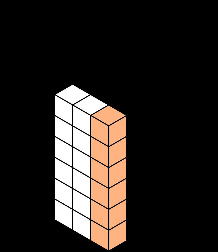
Published as a conference paper at ICLR 2022

                                                            (1)     (2)     (1)     (2)
               Method          ACC      FM       LA       ∆µ      ∆µ      ∆σ 2    ∆σ 2
               Single-BN      72.81    18.65    87.74
                                                         10.85    0.91    3.69    7.74
               Single-BN∗     75.92    15.13    88.24
               ER-BN          80.66     9.34    88.23
                                                          3.56    0.46    1.41    3.16
               ER-BN∗         81.75     8.51    88.46

Table 1: Evaluation metrics on the pMNIST benchmark. The magnitude of the differences are
               (k)      (k)       (k)
calculated as ∆ω = ||ωBN − ωBN ∗ ||1 , where ω ∈ {µ, σ 2 } and k ∈ {1, 2} denotes the first or
second BN layer. Bold indicates the best scores.

GN has shown comparable performance to BN with large mini-batch sizes (e.g. 32 or more), while
significantly outperformed BN with small mini-batch sizes (e.g. one or two). Notably, when putting
all channels into a single group (setting G = 1), GN is equivalent to Layer Normalization (LN) (Ba
et al., 2016), which normalizes the whole layer of each sample. On the other extreme, when separat-
ing each channel as a group (setting G = C), GN becomes Instance Normalization (IN) (Ulyanov
et al., 2016), which normalizes the spatial dimension in each channel of each feature. Figure 1
provides an illustration of BN, GN, IN, and the proposed CN, which we will discuss in Section 4.

3     BATCH N ORMALIZATION IN C ONTINUAL L EARNING
3.1   T HE B ENEFITS OF N ORMALIZATION L AYERS IN C ONTINUAL L EARNING

We argue that BN is helpful for forward transfer in two aspects. First, BN makes the optimization
landscape smoother (Santurkar et al., 2018), which allows the optimization of deep neural networks
to converge faster and better (Bjorck et al., 2018). In continual learning, BN enables the model to
learn individual tasks better than the no-normalization method. Second, with the episodic memory,
BN uses data of the current task and previous tasks (in the memory) to update its running moments.
Therefore, BN further facilitates forward knowledge transfer during experience replay: current task
data is normalized using moments calculated from both current and previous samples. Compared
to BN, spatial normalization layers (such as GN) lack the ability to facilitate forward transfer via
normalizing using moments calculated from data of both old and current tasks. We will empirically
verify the benefits of different normalization layers to continual learning in Section 5.1.

3.2   T HE C ROSS -TASK N ORMALIZATION E FFECT
Recall that BN maintains a running estimate of the global moments to normalize the testing data.
In the standard learning with a single task where data are i.i.d, one can expect such estimates can
well-characterize the true, global moments, and can be used to normalize the testing data. However,
online continual learning data is non-i.i.d and highly non stationary. Therefore, BN’s estimation
of the global moments is heavily biased towards the current task because the recent mini-batches
only contain that task’s data. As a result, during inference, when evaluating the older tasks, BN
normalizes previous tasks’ data using the current task’s moments, which we refer to as the cross-
task normalization effect.
We consider a toy experiment on the permuted MNIST (pMNIST) benchmark (Lopez-Paz & Ran-
zato, 2017) to explore the cross-task normalization effect in BN. We construct a sequence of five task,
each has 2,000 training and 10,000 testing samples, and a multilayer perceptron(MLP) backbone
configured as Input(784)-FC1(100)-BN1(100)-FC2(100)-BN(100)-Softmax(10), where the number
inside the parentheses indicates the output dimension of that layer. We consider the Single and ER
strategies for this experiment, where the Single strategy is the naive method that trains continuously
without any memory or regularization. For each method, we implement an optimal-at-test-time BN
variant (denoted by the suffix -BN∗ ) that calculates the global moments using all training data of
all tasks before testing. Compared to BN, BN∗ has the same parameters and only differs in the
moments used to normalize the testing data. We emphasize that although BN∗ is unrealistic, it sheds
light on how cross-task normalization affects the performance of CL algorithms. We report the av-
eraged accuracy at the end of training ACC(↑) (Lopez-Paz et al., 2017), forgetting measure FM(↓)
(Chaudhry et al., 2018), and learning accuracy LA(↑) (Riemer et al., 2019) in this experiment.

                                                  4
Published as a conference paper at ICLR 2022
Table 1 reports the evaluation metrics of this experiment. Besides the standard metrics, we also
report the moments’ difference magnitudes between the standard BN and the global BN variant.
We observe that the gap between two BN variants is significant without the episodic memory. When
using the episodic memory, ER can reduce the gap because the pMNIST is quite simple and even the
ER strategy can achieve close performances to the offline model (Chaudhry et al., 2019b). Moreover,
it is important to note that training with BN on imbalanced data also affects the model’s learning
dynamics, resulting in a suboptimal parameter. Nevertheless, having an unbiased estimate of the
global moments can greatly improve overall accuracy given the same model parameters. Moreover,
this improvement is attributed to reducing forgetting rather than facilitating transfer: BN∗ has lower
FM but almost similar LA compared to the traditional BN. In addition, we observe that the hidden
features’ variance becomes inaccurate compared to the global variance as we go to deeper layers
(1) (2)
(∆σ2 < ∆σ2 ). This result agrees with recent finding (Ramasesh et al., 2021) that deeper layers are
more responsible for causing forgetting because their hidden representation deviates from the model
trained on all tasks. Overall, these results show that normalizing older tasks using the current task’s
moments causes higher forgetting, which we refer to as the “cross-task normalization effect”.
3.3 D ESIDERATA FOR C ONTINUAL L EARNING N ORMALIZATION L AYERS
While BN facilitates continual learning, it also amplifies catastrophic forgetting by causing the cross-
task normalization effect. To retain the BN’s benefits while alleviating its drawbacks, we argue
that an ideal normalization layer for continual learning should be adaptive by incorporating each
feature’s statistics into its normalization. Being adaptive can mitigate the cross-task normalization
effect because each sample is now normalized differently at test time instead of being normalized
by a set of biased moments. In literature, adaptive normalization layers have shown promising
results when the mini-batch sizes are small (Wu & He, 2018), or when the number of training data is
extremely limited (Bronskill et al., 2020). In such cases, normalizing along the spatial dimensions
of each feature can alleviate the negative effect from an inaccurate estimate of the global moments.
Inspired by this observation, we propose the desiderata for a continual learning normalization layer:
• Facilitates the performance of deep networks by improving knowledge sharing within and
across-task (when the episodic memory is used), thus increasing the performance of all
tasks (ACC in our work);
• Is adaptive at test time: each data sample should be normalized differently. Moreover,
each data sample should contribute to its normalized feature’s statistic, thus reducing catas-
trophic forgetting;
• Does not require additional input at test time such as the episodic memory, or the task
identifier.
To simultaneously facilitate training and mitigating the cross-task normalization effect, a normal-
ization layer has to balance between both across mini-batch normalization and within-sample nor-
malization. As we will show in Section 5.1, BN can facilitate training by normalizing along the
mini-batch dimension; however, it is not adaptive at test time and suffers from the cross-task nor-
malization effect. On the other hand, GN is fully adaptive, but it does not facilitate training compared
to BN. Therefore, it is imperative to balance both aspects to improve continual learning performance.
Lastly, we expect a continual learning normalization layer can be a direct replacement for BN, thus,
it should not require additional information to work, especially at test time.
4 C ONTINUAL N ORMALIZATION (CN)
CN works by first performing a spatial normalization on the feature map, which we choose to be
group normalization. Then, the group-normalized features are further normalized by a batch nor-
malization layer. Formally, given the input feature map a, we denote BN1,0 and GN1,0 as the batch
normalization and group normalization layers without the affine transformation parameters1 , CN
obtains the normalized features aCN as:
aGN ← GN1,0 (a); aCN ← γBN1,0 (aGN ) + β. (6)
1
which is equivalent to setting γ = 1 and β = 0
5Published as a conference paper at ICLR 2022
Table 2: Evaluation metrics of different normalization layers on the Split CIFAR100 and Split Mini
IMN benchmarks. Bold indicates the best averaged scores, † suffix indicates non-adaptive method
ER Split CIFAR100 Split Mini IMN
Norm. Layer ACC(↑) FM(↓) LA(↑) ACC(↑) FM(↓) LA(↑)
NoNL 55.87±0.46 4.46±0.48 57.26±0.64 47.40±2.80 3.17±0.99 45.31±2.18
†
BN 64.97±1.09 9.24±1.98 71.56±0.75 59.09±1.74 8.57±1.52 65.24±0.52
BRN† 63.47±1.33 8.43±1.03 69.83±2.52 54.55±2.70 6.66±1.84 58.53±1.88
IN 59.17±0.96 11.47±0.92 69.40±0.93 48.74±1.98 15.28±1.88 62.88±1.13
GN 63.42±0.92 7.39±1.24 68.03±0.19 55.65±2.92 8.31±1.00 59.25±0.72
SN 64.79±0.88 7.92±0.64 71.10±0.51 56.84±1.37 10.11±1.46 64.09±1.53
CN(ours) 67.48±0.81 7.29±1.59 74.27±0.36 64.28±1.49 8.08±1.18 70.90±1.16
DER++ Split CIFAR100 Split Mini IMN
Norm. Layer ACC(↑) FM(↓) LA(↑) ACC(↑) FM(↓) LA(↑)
NoNL 57.14±0.46 4.46±0.48 57.26±0.64 47.18±3.20 2.77±1.68 45.01±3.35
†
BN 66.50±2.52 8.58±2.28 73.78±1.02 61.08±0.91 6.90±0.99 66.10±0.89
BRN† 66.89±1.22 6.98±2.23 73.30±0.08 57.37±1.75 6.66±1.84 66.53±1.56
IN 61.18±0.96 10.59±0.77 71.00±0.57 54.05±1.26 11.82±1.32 65.03±1.69
GN 66.58±0.27 5.70±0.69 69.63±1.12 60.50±1.91 6.17±1.28 63.10±1.53
SN 67.17±0.23 6.01±0.15 72.13±0.23 57.73±1.97 8.92±1.84 63.87±0.64
CN(ours) 69.13±0.56 6.48±0.81 74.89±0.40 66.29±1.11 6.47±1.46 71.75±0.68
In the first step, our GN component does not use the affine transformation to make the intermediate
feature BN1,0 (aGN ) well-normalized across the mini-batch and spatial dimensions. Moreover, per-
forming GN first allows the spatial-normalized features to contribute to the BN’s running statistic,
which further reduce the cross-task normalization effect. An illustration of CN is given in Figure 1.
By its design, one can see that CN satisfies the desiderata of a continual learning normalization layer.
Particularly, CN balances between facilitating training and alleviating the cross-task normalizing
effect by normalizing the input feature across mini-batch and individually. Therefore, CN is adaptive
at test time and produces well-normalized features in the mini-batch and spatial dimensions, which
strikes a great balance between BN and other instance-based normalizers. Lastly, CN uses the same
input as conventional normalization layers and does not introduce extra learnable parameters that
can be prone to catastrophic forgetting.
We now discuss why CN is a more suitable normalization layer for continual learning than recent
advanced normalization layers. SwitchNorm (Luo et al., 2018) proposed to combine the moments
from three normalization layers: BN, IN, and LN to normalize the feature map (Eq. 13). However,
the blending weights w and w0 make the output feature not well-normalized in any dimensions since
such weights are smaller than one, which scales down the moments. Moreover, the choice of IN and
LN may not be helpful for image recognition problems. Similar to SN, TaskNorm (Bronskill et al.,
2020) combines the moments from BN and IN by a blending factor, which is learned for each task.
As a result, TaskNorm also suffers in that its outputs are not well-normalized. Moreover, TaskNorm
addresses the meta learning problem requires knowing the task identifier at test time, which violates
our third criterion of requiring additional information compared to BN and our CN.
5 E XPERIMENT
We evaluate the proposed CN’s performance compared to a suite of normalization layers with a
focus on the online continual learning settings where it is more challenging to obtain a good global
moments for BN. Our goal is to evaluate the following hypotheses: (i) BN can facilitate knowledge
transfer better than spatial normalization layers such as GN and SN (ii) Spatial normalization layers
have lower forgetting than BN; (iii) CN can improve over other normalization layers by reducing
catastrophic forgetting and facilitating knowledge transfer; (iv) CN is a direct replacement of BN
without additional parameters and minimal computational overhead. Due to space constraints, we
briefly mention the setting before each experiment and provide the full details in Appendix D.
6Published as a conference paper at ICLR 2022
5.1 O NLINE TASK - INCREMENTAL C ONTINUAL L EARNING
Setting We first consider the standard online, task-incremental continual learning setting (Lopez-
Paz & Ranzato, 2017) on the Split CIFAR-100 and Split Mini IMN benchmarks. We follow the
standard setting in Chaudhry et al. (2019a) to split the original CIFAR100 (Krizhevsky & Hinton,
2009) or Mini IMN (Vinyals et al., 2016) datasets into a sequence of 20 tasks, three of which are used
for hyper-parameter cross-validation, and the remaining 17 tasks are used for continual learning.
We consider two continual learning strategies: (i) Experience Replay (ER) (Chaudhry et al., 2019b);
and (ii) Dark Experience Replay++ (DER++) (Buzzega et al., 2020). Besides the vanilla ER, we
also consider DER++, a recent improved ER variants, to demonstrate that our proposed CN can
work well across different ER-based strategies. All methods use a standard ResNet 18 backbone (He
et al., 2016) (not pre-trained) and are optimized over one epoch with batch size 10 using the SGD
optimizer. For each continual learning strategies, we compare our proposed CN with five competing
normalization layers: (i) BN (Ioffe & Szegedy, 2015); (ii) Batch Renormalization (BRN) (Ioffe,
2017); (iii) IN (Ulyanov et al., 2016); (iv) GN (Wu & He, 2018); and (v) SN (Luo et al., 2018). We
cross-validate and set the number of groups to be G = 32 for our CN and GN in this experiment.
Results Table 2 reports the evaluation metrics of different normalization layers on the Split
CIFAR-100 and Split Mini IMN benchmarks. We consider the averaged accuracy at the end of
training ACC(↑) (Lopez-Paz et al., 2017), forgetting measure FM(↓) (Chaudhry et al., 2018), and
learning accuracy LA(↑) (Riemer et al., 2019), details are provided in Appendix A. Clearly, IN
does not perform well because it is not designed for image recognition problems. Compared to
adaptive normalization methods such as GN and SN, BN suffers from more catastrophic forgetting
(higher FM(↓) ) but at the same time can transfer knowledge better across tasks (higher LA(↑) ).
Moreover, BRN performs worse than BN since it does not address the biased estimate of the global
moments, which makes normalizing with the global moments during training ineffective. Overall,
the results show that although traditional adaptive methods such as GN and SN do not suffer from
the cross-task normalization effect and enjoy lower FM(↓) values, they lack the ability to facilitate
knowledge transfer across tasks, which results in lower LA(↑) . Moreover, BN can facilitate knowl-
edge sharing across tasks, but it suffers more from forgetting because of the cross-task normalization
effect. Across all benchmarks, our CN comes out as a clear winner by achieving the best overall
performance (ACC(↑) ). This result shows that CN can strike a great balance between reducing
catastrophic forgetting and facilitating knowledge transfer to improve continual learning.
Complexity Comparison We study the com-
plexity of different normalization layers and Table 3: Running time of ER on the Split CI-
reporting the training time on the Split CI- FAR100 benchmarks of different normalization
FAR100 benchmark in Tabe 3. Both GN and layers. ∆% indicates the percentage increases of
our CN have minimal computational overhead training time over BN
compared to BN, while SN suffers from addi-
tional computational cost from calculating and BN GN SN CN
normalizing with different sets of moments. Time (s) 1583 1607 2036 1642
∆% 0% 1.51% 28.61% 3.72%
5.2 O NLINE C LASS -I NCREMENTAL
C ONTINUAL L EARNING
Setting We consider the online task incremental (Task-IL) and class incremental (Class-IL) learn-
ing problems on the Split-CIFAR10 (Split CIFAR-10) and Split-Tiny-ImageNet (Split Tiny IMN)
benchmarks. We follow the same experiment setups as Buzzega et al. (2020) except the number of
training epochs, which we set to one. All experiments uses the DER++ strategy (Buzzega et al.,
2020) on a ResNet 18 (He et al., 2016) backbone (not pre-trained) trained with data augmentation
using the SGD optimizer. We consider three different total episodic memory sizes of 500, 2560, and
5120, and focus on comparing BN with our proposed CN in this experiment.
Result Table 4 reports the ACC and FM metrics on the Split CIFAR-10 and Split Tiny IMN bench-
marks under both the Task-IL and Class-IL settings. For CN, we consider two configurations with
the number of groups being G = 8 and G = 32. In most cases, our CN outperforms the standard BN
on both metrics, with a more significant gap on larger memory sizes of 2560 and 5120. Interestingly,
BN is highly unstable in the Split CIFAR-10, Class-IL benchmark with high standard deviations. In
7Published as a conference paper at ICLR 2022
Table 4: Evaluation metrics of DER++ with different normalization layers on the Split CIFAR-10
and Split Tiny IMN benchmarks. Parentheses indicates the number of groups in CN. Bold indicates
the best averaged scores
Split CIFAR-10 Split Tiny IMN
Buffer Method
Class-IL Task-IL Class-IL Task-IL
ACC(↑) FM(↓) ACC(↑) FM(↓) ACC(↑) FM(↓) ACC(↑) FM(↓)
BN 48.9±4.5 33.6±5.8 82.6±2.3 3.2±1.9 6.7±0.1 38.1±0.5 40.2±0.9 6.5±1.0
500 CN (G = 8) 48.9±0.3 27.9±5.0 84.7±0.5 2.2±0.3 7.3±0.9 37.5±2.3 42.2±2.1 4.9±2.2
CN (G = 32) 51.7±1.9 28.2±4.0 86.2±2.2 2.0±1.3 6.5±0.7 40.1±1.7 40.6±1.4 6.8±1.9
BN 52.3±4.6 29.7±6.1 86.6±1.6 0.9±0.7 11.2±2.3 36.0±2.0 50.8±1.7 2.8±1.2
2560 CN (G = 8) 53.7±3.4 25.5±4.7 87.3±2.7 1.6±1.6 10.7±1.3 38.0±1.2 52.6±1.2 1.5±0.5
CN (G = 32) 57.3±2.0 21.6±5.6 88.4±1.1 1.7±1.1 11.9±0.3 36.7±1.2 51.5±0.2 2.8±0.9
BN 52.0±7.8 26.7±10.3 85.6±3.3 2.0±1.5 11.2±2.7 36.8±2.0 52.2±1.7 2.6±1.5
5120 CN (G = 8) 54.1±4.0 24.0±4.0 87.1±2.8 0.7±0.7 12.2±0.6 34.6±2.6 53.1±1.8 3.1±1.9
CN (G = 32) 57.9±4.1 22.2±1.0 88.3±0.9 1.3±0.9 12.2±0.2 35.6±1.3 54.9±1.5 1.5±1.1
90
50
85
ACC
ACC
40
80 CN(G=32) CN(G=32)
CN(G=8) CN(G=8)
BN 30 BN
75
1 2 3 4 5 1 2 3 4 5 6 7 8 9 10
Task Task
(a) Split CIFAR-10, Task-IL (b) Split Tiny IMN, Task-IL
Figure 2: The evolution of ACC(↑) on observed tasks so far on the Split CIFAR-10 and Split Tiny
IMN benchmarks, Task-IL screnario with DER++ and memory size of 5120 samples.
contrast, both CN variants show better and more stable results, especially in the more challenging
Class-IL setting with a small memory size (indicated by small standard deviation values). We also
report the evolution of ACC in Figure 2. Both CN variants consistently outperform BN throughout
training, with only one exception at the second task on the Split Tiny IMN. CN (G = 32) shows
more stable and better performances than BN and CN(G = 8).
5.3 L ONG - TAILED O NLINE C ONTINUAL L EARNING
We now evaluate the normalization layers on the challenging task-free, long-tailed continual learn-
ing setting (Kim et al., 2020), which is more challenging and realistic since real-world data usually
follow long-tailed distributions. We consider the PRS strategy (Kim et al., 2020) and the COCOseq
and NUS-WIDEseq benchmarks, which consists of four and six tasks, respectively. Unlike the previ-
ous benchmarks, images in the COCOseq and NUS-WIDEseq benchmarks can have multiple labels,
resulting in a long-tailed distribution over each task’s image label. Following Kim et al. (2020), we
report the average overall F1 (O-F1), per-class F1 (C-F1), and the mean average precision (mAP)
at the end of training and their corresponding forgetting measures (FM). We also report each metric
over the minority classes (900 samples), and all classes. Empirically, we found that smaller groups helped in the long-tailed
setting because the moments were calculated over more channels, reducing the dominants of head
classes. Therefore, we use G = 4 groups in this experiment.
We replicate PRS with BN to compare with our CN and report the results in Table 5 and Table 6. We
observe consistent improvements over BN from only changing the normalization layers, especially
in reducing FM(↓) across all classes.
8Published as a conference paper at ICLR 2022
Table 5: Evaluation metrics of the PRS strategy on the COCOseq and NUS-WIDEseq benchmarks.
We report the mean performance over five runs. Bold indicates the best averaged scores
Majority Moderate Minority Overall
COCOseq
C-F1 O-F1 mAP C-F1 O-F1 mAP C-F1 O-F1 mAP C-F1 O-F1 mAP
BN 64.2 58.3 66.2 51.2 48.1 55.7 31.6 31.4 38.1 51.8 48.6 54.9
CN(ours) 64.8 58.5 66.8 52.5 49.2 55.7 35.7 35.5 38.4 53.1 49.8 55.1
Majority Moderate Minority Overall
NUS-WIDEseq
C-F1 O-F1 mAP C-F1 O-F1 mAP C-F1 O-F1 mAP C-F1 O-F1 mAP
BN 24.3 16.1 21.2 16.2 16.5 20.9 28.5 28.2 32.3 23.4 20.9 25.7
CN(ours) 25.0 17.2 22.7 17.1 17.4 21.5 27.3 27.0 31.0 23.5 21.3 25.9
Table 6: Forgetting measure (FM(↓) ) of each metric from the PRS strategy on the COCOseq and
NUS-WIDEseq benchmarks, lower is better. We report the mean performance over five runs. Bold
indicates the best averaged scores
Majority Moderate Minority Overall
COCOseq
C-F1 O-F1 mAP C-F1 O-F1 mAP C-F1 O-F1 mAP C-F1 O-F1 mAP
BN 23.5 22.8 8.4 30.0 30.2 9.4 36.2 35.7 13.2 29.7 29.5 9.7
CN(ours) 23.5 23.1 6.5 26.9 26.9 7.4 26.8 26.5 12.2 25.6 25.7 8.0
Majority Moderate Minority Overall
NUS-WIDEseq
C-F1 O-F1 mAP C-F1 O-F1 mAP C-F1 O-F1 mAP C-F1 O-F1 mAP
BN 54.6 50.7 12.5 62.2 61.9 15.5 52.5 52.4 12.2 57.6 55.7 11.2
CN(ours) 52.7 48.7 8.6 58.8 58.0 10.3 51.2 50.6 11.6 57.4 55.5 8.1
5.4 D ISCUSSION OF T HE R ESULTS
Our experiments have shown promising results for CN being a potential replacement for BN in on-
line continual learning. While the results are generally consistent, there are a few scenarios where
CN does not perform as good as other baselines. First, from the task-incremental experiment in Ta-
ble 2, DER++ with CN achieved lower FM compared to GN. The reason could be from the DER++’s
soft-label loss, which together with GN, overemphasizes on reducing FM and achieved lower FM.
On the other hand, CN has to balance between reducing FM and improving LA. Second, training
with data augmentation in the online setting could induce high variations across different runs. Ta-
ble 4 shows that most methods have high standard deviations on the Split CIFAR-10 benchmark,
especially with small memory sizes. In such scenarios, there could be insignificant differences be-
tween the first and second best methods. Also, on the NUS-WIDEseq benchmark, CN has lower
evaluation metrics on minority classes than BN. One possible reason is the noisy nature of the NUS-
WIDE dataset, including the background diversity and huge number of labels per image, which could
highly impact the tail classes’ performance. Lastly, CN introduces an additional hyper-parameter
(number of groups), which needs to be cross-validated for optimal performance.
6 C ONCLUSION
In this paper, we investigate the potentials and limitations of BN in online continual learning, which
is a common component in most existing methods but has not been actively studied. We showed
that while BN can facilitate knowledge transfer by normalizing along the mini-batch dimension, the
cross-task normalization effect hinders older tasks’ performance and increases catastrophic forget-
ting. This limitation motivated us to propose CN, a novel normalization layer especially designed for
online continual learning settings. Our extensive experiments corroborate our findings and demon-
strate the efficacy of CN over other normalization strategies. Particularly, we showed that CN is a
plug-in replacement for BN and can offer significant improvements on different evaluation metrics
across different online settings with minimal computational overhead.
9Published as a conference paper at ICLR 2022
ACKNOWLEDGEMENT
The first author is supported by the SMU PGR scholarship. We thank the anonymous Reviewers for
the constructive feedback during the submission of this work.
E THIC S TATEMENT
No human subjects were involved during the research and developments of this work. All of our
experiments were conducted on the standard benchmarks in the lab-based, controlled environment.
Thus, due to the abstract nature of this work, it has minimal concerns regarding issues such as
discrimination/bias/fairness, privacy, etc.
R EPRODUCIBILITY S TATEMENT
In this paper, we conduct the experiments five times and report the mean and standard deviation
values to alleviate the randomness of the starting seed. In Appendix D, we provide the full details
of our experimental settings.
R EFERENCES
Wickliffe C Abraham and Anthony Robins. Memory retention–the synaptic stability versus plastic-
ity dilemma. Trends in neurosciences, 28(2):73–78, 2005.
Rahaf Aljundi, Francesca Babiloni, Mohamed Elhoseiny, Marcus Rohrbach, and Tinne Tuytelaars.
Memory aware synapses: Learning what (not) to forget. In Proceedings of the European Confer-
ence on Computer Vision (ECCV), pp. 139–154, 2018.
Rahaf Aljundi, Eugene Belilovsky, Tinne Tuytelaars, Laurent Charlin, Massimo Caccia, Min Lin,
and Lucas Page-Caccia. Online continual learning with maximal interfered retrieval. In Advances
in Neural Information Processing Systems, pp. 11849–11860, 2019a.
Rahaf Aljundi, Klaas Kelchtermans, and Tinne Tuytelaars. Task-free continual learning. In Pro-
ceedings of the IEEE Conference on Computer Vision and Pattern Recognition, pp. 11254–11263,
2019b.
Jimmy Lei Ba, Jamie Ryan Kiros, and Geoffrey E Hinton. Layer normalization. arXiv preprint
arXiv:1607.06450, 2016.
Johan Bjorck, Carla Gomes, Bart Selman, and Kilian Q Weinberger. Understanding batch normal-
ization. In Proceedings of the 32nd International Conference on Neural Information Processing
Systems, pp. 7705–7716, 2018.
Andrew Brock, Soham De, and Samuel L Smith. Characterizing signal propagation to close the
performance gap in unnormalized resnets. arXiv preprint arXiv:2101.08692, 2021.
John Bronskill, Jonathan Gordon, James Requeima, Sebastian Nowozin, and Richard Turner. Tas-
knorm: Rethinking batch normalization for meta-learning. In International Conference on Ma-
chine Learning, pp. 1153–1164. PMLR, 2020.
Pietro Buzzega, Matteo Boschini, Angelo Porrello, Davide Abati, and Simone Calderara. Dark
experience for general continual learning: a strong, simple baseline. In 34th Conference on
Neural Information Processing Systems (NeurIPS 2020), 2020.
Arslan Chaudhry, Puneet K Dokania, Thalaiyasingam Ajanthan, and Philip HS Torr. Riemannian
walk for incremental learning: Understanding forgetting and intransigence. In Proceedings of the
European Conference on Computer Vision (ECCV), pp. 532–547, 2018.
Arslan Chaudhry, Marc’Aurelio Ranzato, Marcus Rohrbach, and Mohamed Elhoseiny. Efficient
lifelong learning with a-gem. International Conference on Learning Representations (ICLR),
2019a.
10Published as a conference paper at ICLR 2022
Arslan Chaudhry, Marcus Rohrbach, Mohamed Elhoseiny, Thalaiyasingam Ajanthan, Puneet K
Dokania, Philip HS Torr, and Marc’Aurelio Ranzato. On tiny episodic memories in continual
learning. arXiv preprint arXiv:1902.10486, 2019b.
Robert M French. Catastrophic forgetting in connectionist networks. Trends in cognitive sciences,
3(4):128–135, 1999.
Kaiming He, Xiangyu Zhang, Shaoqing Ren, and Jian Sun. Deep residual learning for image recog-
nition. In Proceedings of the IEEE conference on computer vision and pattern recognition, pp.
770–778, 2016.
Lei Huang, Jie Qin, Yi Zhou, Fan Zhu, Li Liu, and Ling Shao. Normalization techniques in training
dnns: Methodology, analysis and application. arXiv preprint arXiv:2009.12836, 2020.
Sergey Ioffe. Batch renormalization: towards reducing minibatch dependence in batch-normalized
models. In Proceedings of the 31st International Conference on Neural Information Processing
Systems, pp. 1942–1950, 2017.
Sergey Ioffe and Christian Szegedy. Batch normalization: Accelerating deep network training by
reducing internal covariate shift. In International conference on machine learning, pp. 448–456.
PMLR, 2015.
Khurram Javed and Faisal Shafait. Revisiting distillation and incremental classifier learning. In
Asian conference on computer vision, pp. 3–17. Springer, 2018.
Chris Dongjoo Kim, Jinseo Jeong, and Gunhee Kim. Imbalanced continual learning with partition-
ing reservoir sampling. In European Conference on Computer Vision, pp. 411–428. Springer,
2020.
Diederik P Kingma and Jimmy Ba. Adam: A method for stochastic optimization. arXiv preprint
arXiv:1412.6980, 2014.
James Kirkpatrick, Razvan Pascanu, Neil Rabinowitz, Joel Veness, Guillaume Desjardins, Andrei A
Rusu, Kieran Milan, John Quan, Tiago Ramalho, Agnieszka Grabska-Barwinska, et al. Overcom-
ing catastrophic forgetting in neural networks. Proceedings of the national academy of sciences,
2017.
Alex Krizhevsky and Geoffrey Hinton. Learning multiple layers of features from tiny images. Tech-
nical report, Citeseer, 2009.
Yann LeCun, Léon Bottou, Yoshua Bengio, and Patrick Haffner. Gradient-based learning applied to
document recognition. Proceedings of the IEEE, 86(11):2278–2324, 1998.
Yann LeCun, Yoshua Bengio, and Geoffrey Hinton. Deep learning. nature, 521(7553):436–444,
2015.
Xilai Li, Yingbo Zhou, Tianfu Wu, Richard Socher, and Caiming Xiong. Learn to grow: A continual
structure learning framework for overcoming catastrophic forgetting. In International Conference
on Machine Learning, pp. 3925–3934, 2019.
Long-Ji Lin. Self-improving reactive agents based on reinforcement learning, planning and teaching.
Machine learning, 8(3-4):293–321, 1992.
Vincenzo Lomonaco, Davide Maltoni, and Lorenzo Pellegrini. Rehearsal-free continual learning
over small non-iid batches. In CVPR Workshops, pp. 989–998, 2020.
David Lopez-Paz and Marc’Aurelio Ranzato. Gradient episodic memory for continual learning. In
Advances in Neural Information Processing Systems, pp. 6467–6476, 2017.
David Lopez-Paz, Robert Nishihara, Soumith Chintala, Bernhard Scholkopf, and Léon Bottou. Dis-
covering causal signals in images. In Proceedings of the IEEE Conference on Computer Vision
and Pattern Recognition, pp. 6979–6987, 2017.
11Published as a conference paper at ICLR 2022
Ping Luo, Jiamin Ren, Zhanglin Peng, Ruimao Zhang, and Jingyu Li. Differentiable learning-to-
normalize via switchable normalization. In International Conference on Learning Representa-
tions, 2018.
Cuong V Nguyen, Yingzhen Li, Thang D Bui, and Richard E Turner. Variational continual learning.
International Conference on Learning Representations (ICLR), 2018.
German I Parisi, Ronald Kemker, Jose L Part, Christopher Kanan, and Stefan Wermter. Continual
lifelong learning with neural networks: A review. Neural Networks, 2019.
Adam Paszke, Sam Gross, Soumith Chintala, Gregory Chanan, Edward Yang, Zachary DeVito,
Zeming Lin, Alban Desmaison, Luca Antiga, and Adam Lerer. Automatic differentiation in
pytorch. In NIPS-W, 2017.
Quang Pham, Chenghao Liu, Doyen Sahoo, et al. Contextual transformation networks for online
continual learning. In International Conference on Learning Representations, 2020.
Quang Pham, Chenghao Liu, and Steven Hoi. Dualnet: Continual learning, fast and slow. Advances
in Neural Information Processing Systems, 34, 2021.
Vinay V Ramasesh, Ethan Dyer, and Maithra Raghu. Anatomy of catastrophic forgetting: Hidden
representations and task semantics. In International Conference on Learning Representations,
2021.
Sylvestre-Alvise Rebuffi, Alexander Kolesnikov, Georg Sperl, and Christoph H Lampert. icarl:
Incremental classifier and representation learning. In Proceedings of the IEEE conference on
Computer Vision and Pattern Recognition, pp. 2001–2010, 2017.
Matthew Riemer, Ignacio Cases, Robert Ajemian, Miao Liu, Irina Rish, Yuhai Tu, and Gerald
Tesauro. Learning to learn without forgetting by maximizing transfer and minimizing interfer-
ence. International Conference on Learning Representations (ICLR), 2019.
Mark B Ring. Child: A first step towards continual learning. Machine Learning, 28(1):77–104,
1997.
Hippolyt Ritter, Aleksandar Botev, and David Barber. Online structured laplace approximations for
overcoming catastrophic forgetting. In Advances in Neural Information Processing Systems, pp.
3738–3748, 2018.
David Rolnick, Arun Ahuja, Jonathan Schwarz, Timothy Lillicrap, and Gregory Wayne. Experience
replay for continual learning. In Advances in Neural Information Processing Systems, pp. 348–
358, 2019.
Andrei A Rusu, Neil C Rabinowitz, Guillaume Desjardins, Hubert Soyer, James Kirkpatrick, Koray
Kavukcuoglu, Razvan Pascanu, and Raia Hadsell. Progressive neural networks. arXiv preprint
arXiv:1606.04671, 2016.
Shibani Santurkar, Dimitris Tsipras, Andrew Ilyas, and Aleksander Madry. How does batch nor-
malization help optimization? In Proceedings of the 32nd International Conference on Neural
Information Processing Systems, pp. 2488–2498, 2018.
Joan Serra, Didac Suris, Marius Miron, and Alexandros Karatzoglou. Overcoming catastrophic
forgetting with hard attention to the task. In Proceedings of the 35th International Conference on
Machine Learning-Volume 80, pp. 4548–4557. JMLR. org, 2018.
Dmitry Ulyanov, Andrea Vedaldi, and Victor Lempitsky. Instance normalization: The missing in-
gredient for fast stylization. arXiv preprint arXiv:1607.08022, 2016.
Dmitry Ulyanov, Andrea Vedaldi, and Victor Lempitsky. Improved texture networks: Maximizing
quality and diversity in feed-forward stylization and texture synthesis. In Proceedings of the IEEE
Conference on Computer Vision and Pattern Recognition, pp. 6924–6932, 2017.
Oriol Vinyals, Charles Blundell, Timothy Lillicrap, Daan Wierstra, et al. Matching networks for one
shot learning. In Advances in neural information processing systems, pp. 3630–3638, 2016.
12Published as a conference paper at ICLR 2022
Johannes von Oswald, Christian Henning, João Sacramento, and Benjamin F Grewe. Continual
learning with hypernetworks. International Conference on Learning Representations (ICLR),
2020.
Yue Wu, Yinpeng Chen, Lijuan Wang, Yuancheng Ye, Zicheng Liu, Yandong Guo, and Yun Fu.
Large scale incremental learning. In Proceedings of the IEEE/CVF Conference on Computer
Vision and Pattern Recognition, pp. 374–382, 2019.
Yuxin Wu and Kaiming He. Group normalization. In Proceedings of the European conference on
computer vision (ECCV), pp. 3–19, 2018.
Jingjing Xu, Xu Sun, Zhiyuan Zhang, Guangxiang Zhao, and Junyang Lin. Understanding and
improving layer normalization. arXiv preprint arXiv:1911.07013, 2019.
Ju Xu and Zhanxing Zhu. Reinforced continual learning. In Advances in Neural Information Pro-
cessing Systems, pp. 899–908, 2018.
Jaehong Yoon, Eunho Yang, Jeongtae Lee, and Sung Ju Hwang. Lifelong learning with dynamically
expandable networks. International Conference on Learning Representations (ICLR), 2018.
Friedemann Zenke, Ben Poole, and Surya Ganguli. Continual learning through synaptic intelligence.
In Proceedings of the 34th International Conference on Machine Learning-Volume 70, pp. 3987–
3995. JMLR. org, 2017.
A PPENDIX O RGANIZATION
The Appendix of this work is organized as follows. In Appendix A we detail the evaluation metrics
used in our experiments. We provide the details of additional normalization layers that we compared
in our experiments in Appendix B. In Appendix C, we discuss how our results related to existing
studies. Next, Appendix D provides additional details regarding our experiments, including the
information of the benchmarks and additional ablation studies. Lastly, we conclude this work with
the implementation in Appendix E.
A E VALUATION M ETRICS
For a comprehensive evaluation, we use three standard metrics to measure the model’s performance:
Average Accuracy (Lopez-Paz & Ranzato, 2017), Forgetting Measure (Chaudhry et al., 2018), and
Learning Accuracy (Riemer et al., 2019). Let ai,j be the model’s accuracy evaluated on the test set
of task Tj after it finished learning the task Ti . The aforementioned metrics are defined as:
• Average Accuracy (higher is better):
T
1X
ACC(↑) = aT,i . (7)
T i=1
• Forgetting Measure (lower is better):
T −1
1 X
FM(↓) = max al,j − aT,j . (8)
T − 1 j=1 l∈{1,...T −1}
• Learning Accuracy (higher is better):
T
1X
LA(↑) = ai,i . (9)
T i=1
The Averaged Accuracy (ACC) measures the model’s overall performance across all tasks and is
a common metric to compare among different methods. Forgetting Measure (FM) measures the
model’s forgetting as the averaged performance degrades of old tasks. Finally, Learning Accuracy
(LA) measures the model’s ability to acquire new knowledge. Note that in the task free setting, the
task identifiers are not given to the model at any time and are only used to measure the evaluation
metrics.
13Published as a conference paper at ICLR 2022
B A DDITIONAL N ORMALIZATION L AYERS
This section covers the additional normalization layers used in our experiments.
B.1 L AYER N ORMALIZATION (LN)
Layer Normalization Ba et al. (2016) was proposed to address the discrepancy between training and
testing in BN by normalization along the spatial dimension of the input feature. Particularly, LN
computes the moments to normalize the activation as:
C W H
1 XXX
µLN = abcwh
CW H c=1 w=1
h=1
C X
W X
H
2 1 X
σLN = (abcwh − µLN )2 (10)
CW H c=1 w=1 h=1
B.2 I NSTANCE N ORMALIZATION (IN)
Similar to LN, Instance Normalization Ulyanov et al. (2016) also normalizes along the spatial di-
mension. However, IN normalizes each channel separately instead of jointly as in LN. Specifically,
IN computes the moments to normalize as:
W H
1 XX
µIN = abcwh
W H w=1
h=1
H
W X
2 1 X
σIN = (abcwh − µLN )2 (11)
WH w=1 h=1
B.3 BATCH R ENORMALIZATION (BRN)
Batch Renormalization Ioffe (2017) was proposed to alleviate the non-i.i.d or small batches in the
training data. BRN proposed to normalize training data using the running moments estimated so far
by the following re-parameterization trick:
a − µBN
aBRN = γ r +d +β (12)
σBN +
where
σBN
r =stop grad clip[1/rmax ,rmax ]
σr
µBN − µr
d =stop grad clip[−dmax ,dmax ] ,
σr
where stop grad denotes a gradient blocking operation where its arguments are treated as con-
stant during training and the gradient is not back-propagated through them.
B.4 S WITCHABLE N ORMALIZATION (SN)
While LN and IN addressed some limitations of BN, their success are quite limited to certain applica-
tions. For example, LR is suitable for recurrent neural networks and language applications (Ba et al.,
2016; Xu et al., 2019), while IN is widely used in image stylization and image generation (Ulyanov
et al., 2016; 2017). Beyond their dedicated applications, BN still performs superior to LR and IN.
Therefore, SN (Luo et al., 2018) is designed to take advantage of both LN and IN while enjoying
BN’s strong performance. Let Ω = {BN,LN,IN} , SN combines the moments of all three normal-
ization layers and performs the following normalization:
P !
0 a − k∈Ω wµk
a =γ p + β, (13)
w0 σk2 +
14Published as a conference paper at ICLR 2022
Table 7: Dataset summary
#task img size #training imgs #testing imgs #classes Section
pMNIST 5 28×28 10,000 50,000 10 Section 3.2
Split CIFAR10 5 3×32×32 50,000 10,000 10 Section 5.2
Split CIFAR100 20 3×84×84 50,000 10,000 100 Section 5.1
Split Mni IMN 20 3×84×84 50,000 10,000 100 Section 5.1
Split Tiny IMN 10 3×64×64 100,000 10,000 200 Section 5.2
COCOseq 4 3×224×224 35,072 6,346 70 Section 5.3
NUS-WIDEseq 6 3×224×224 48,724 2,367 49 Section 5.3
where w and w0 are the learned blending factors to combine the three moments and are learned by
backpropagation.
C E XISTING REMEDIES FOR THE CROSS - TASK NORMALIZATION EFFECT
From Table 1, we can see that the performance gap between BN and BN∗ is much smaller in ER
compared to the Single method. Since ER employs an episodic memory, its moments are estimated
from both the current data and a small subset of previous memory data. However, there still exists
a gap compared to the optimal BN’s moments, as shown by large ∆µ and ∆σ2 values. In litera-
ture, there exist efforts to such as herding (Rebuffi et al., 2017) and coreset (Nguyen et al., 2018)
to maintain a smaller subset of samples that produces the same feature mean (first moment) as the
original data. However, empirically they provide insignificant improvements over the random sam-
pling strategies (Javed & Shafait, 2018; Chaudhry et al., 2019a). We can explain this result by the
internal covariate shift property in BN: a coreset selected to match the whole dataset’s feature mean
is corresponding to the network parameters producing such features. After learning a new task, the
network parameters are changed to obtain new knowledge and become incompatible with the coreset
constructed using the previous parameters. Unfortunately, we cannot fully avoid this negative effect
without storing all previous data. With limited episodic memory, lost samples will never contribute
to the global moments estimated by the network parameters trained on newer tasks.
D A DDITIONAL E XPERIMENTS
D.1 DATASET S UMMARY
Table 7 summaries the datasets used throughout our experiments.
D.2 E XPERIMENT S ETTINGS
This section details the experiment settings in our work.
Toy pMNIST Benchmark In the toy pMNIST benchmark, we construct a sequence of five task
by applying a random but fixed permutation on the original MNIST LeCun et al. (1998) dataset to
create a task. Each task consists of 1,000 training samples and 10,000 testing samples as the original
MNIST dataset. In the pre-processing step, we normalize the pixel value by dividing its value by
255.0. Both the Single and Experience Replay (ER) methods were trained using the Stochastic
Gradient Descent (SGD) optimizer with mini-batch size 10 over one epoch with learning rate 0.03.
This benchmark follows the “single-head” setting Chaudhry et al. (2018), thus we only maintain a
single classifier for all tasks and task-identifiers are not provided in both training and testing.
Online Task-IL Continual Learning Benchmarks (Split CIFAR100 and Split Mini IMN) In
the data pre-processing step, we normalize the pixel density to [0−1] range and resize the image size
to 3 × 32 × 32 and 3 × 84 × 84 for the Split CIFAR100 and Split minIMN benchmarks, respectively.
No other data pre-processing steps are performed. All methods are optimized by SGD with mini-
batch size 10 over one epoch. The episodic memory is implemented as a Ring buffer Chaudhry et al.
(2019a) with 50 samples per task.
15You can also read