Characteristics of two tsunamis generated by successive Mw 7.4 and Mw 8.1 earthquakes in the Kermadec Islands on 4 March 2021
←
→
Page content transcription
If your browser does not render page correctly, please read the page content below
Nat. Hazards Earth Syst. Sci., 22, 1073–1082, 2022
https://doi.org/10.5194/nhess-22-1073-2022
© Author(s) 2022. This work is distributed under
the Creative Commons Attribution 4.0 License.
Characteristics of two tsunamis generated by successive Mw 7.4
and Mw 8.1 earthquakes in the Kermadec Islands on 4 March 2021
Yuchen Wang1,2 , Mohammad Heidarzadeh3,4 , Kenji Satake1 , and Gui Hu5
1 EarthquakeResearch Institute, The University of Tokyo, Tokyo, 113-0032, Japan
2 JapanAgency for Marine–Earth Science and Technology, Kanazawa, Yokohama, 236-0001, Japan
3 Department of Civil and Environmental Engineering, Brunel University London, Uxbridge, UB8 3PH, UK
4 Department of Architecture and Civil Engineering, University of Bath, Bath BA2 7AY, UK
5 Guangdong Provincial Key Laboratory of Geodynamics and Geohazards, School of Earth Sciences and Engineering,
Sun Yat-Sen University, Guangzhou, 510275, China
Correspondence: Yuchen Wang (ywang@jamstec.go.jp)
Received: 1 December 2021 – Discussion started: 2 December 2021
Revised: 8 February 2022 – Accepted: 10 March 2022 – Published: 1 April 2022
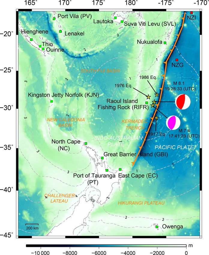
Abstract. On 4 March 2021, two tsunamigenic earth- ards in New Zealand (e.g., Power et al., 2012). The historical
quakes (Mw 7.4 and Mw 8.1) occurred successively within records of earthquakes in the Kermadec Islands are short, but
2 h in the Kermadec Islands, offshore New Zealand. We ex- there were three great earthquakes over the 20th century: the
amined sea level records at tide gauges located at ∼ 100 to ∼ 1917 (Mw 8.6; Morgan, 1918), the 1976 (Mw 8.0; Wyss et
2000 km from the epicenters, conducted Fourier and wavelet al., 1984), and the 1986 earthquakes (Mw 7.9; Lundgren et
analyses as well as numerical modeling of both tsunamis. al., 1989).
Fourier analyses indicated that the energy of the first tsunami On 4 March 2021, two earthquakes occurred successively
is mainly distributed over the period range of 5–17 min, in the Kermadec Islands. The first event (Mw 7.4; fore-
whereas it is 8–32 min for the second tsunami. Wavelet plots shock) occurred at 17:41:23 UTC, whose epicenter was at
showed that the oscillations of the first tsunami continued 29.677◦ S, 177.840◦ W, south of Raoul Island in the Ker-
even after the arrival of the second tsunami. As the epicen- madec Islands region with a depth of 43.0 km (United
ters of two earthquakes are close to each other (∼ 55 km), we States Geological Survey – USGS; https://earthquake.usgs.
reconstructed the source spectrum of the second tsunami by gov/earthquakes/eventpage/us7000dfk3/executive, last ac-
using the first tsunami as the empirical Green’s function. The cess: 4 June 2021) (Fig. 1). The earthquake generated a small
main spectral peaks are 25.6, 16.0, and 9.8 min. The results tsunami. The second earthquake (Mw 8.1; mainshock) oc-
are similar to those calculated using tsunami-to-background curred at 19:28:33 UTC, approximately 2 h after the fore-
ratio method and are also consistent with the source models. shock. The epicenter was located at 29.723◦ S, 177.279◦ W
with a depth of 28.9 km (USGS). The epicenters of these
two successive tsunamigenic earthquakes are very close
to each other (∼ 55 km; Fig. 1) and their focal mecha-
1 Introduction nisms are similar; both are thrust earthquakes. The National
Emergency Management Agency, New Zealand, issued a
The Kermadec Islands are an island arc in the southwest- tsunami warning for coastal areas of the North Island af-
ern Pacific Ocean, formed at the convergent boundary where ter the Mw 8.1 earthquake. The tsunami propagated across
the Pacific Plate subducts under the Indo-Australian Plate the Pacific Ocean and reached South America. No casual-
(Fig. 1) (Billen et al., 2003). The Kermadec Trench, which ties were reported. The situation of these two consequent
accommodates westward subduction of the Pacific Plate be- tsunamigenic earthquakes resembles the earthquake events
neath the active Kermadec volcanic arc, is identified as the also in the Kermadec Islands on 14 January 1976, where
key region for concern regarding seismic and tsunami haz-
Published by Copernicus Publications on behalf of the European Geosciences Union.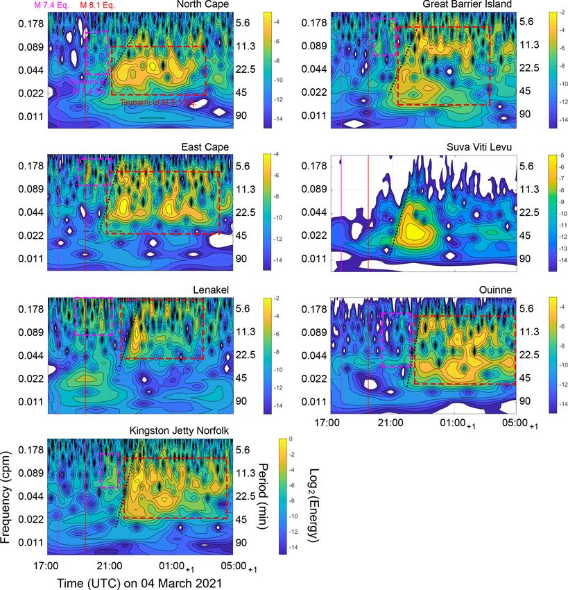
1074            Y. Wang et al.: Characteristics of two tsunamis generated by successive M w 7.4 and M w 8.1 earthquakes

                                                                    tion can be readily made for two successive tsunami events
                                                                    in the Kermadec Islands. If the sources of two earthquakes
                                                                    are close to each other, we can adopt the method of empiri-
                                                                    cal Green’s function (EGF) to reconstruct the tsunami source
                                                                    spectrum (Heidarzadeh et al., 2016). The smaller tsunami
                                                                    event is adopted as the EGF for the larger one. The spectral
                                                                    deconvolution separates the effects of propagation path and
                                                                    local topography around the tide gauge and gives the source
                                                                    spectrum of the larger tsunami. Heidarzadeh et al. (2016)
                                                                    successfully applied the EGF method to the 2015 (Mw 7.0)
                                                                    and 2013 (Mw 8.0) earthquakes in the Solomon Islands.
                                                                       Here, we studied the characteristics of tsunamis generated
                                                                    by the two successive Kermadec Islands earthquakes and cal-
                                                                    culated the source spectrum of the tsunami generated by the
                                                                    mainshock (hereafter, the second tsunami). Fourier analysis
                                                                    was applied to the sea level records at 15 tide gauges. Wavelet
                                                                    analysis was adopted to examine the temporal changes of
                                                                    the dominant spectral peaks. Finally, we used two differ-
                                                                    ent methods, tsunami-to-background spectral ratio method
                                                                    and EGF method, to reconstruct tsunami source spectra. We
                                                                    compared two alternative methods of determining tsunami
                                                                    source spectra and also compared their results with USGS
                                                                    source models. This is a unique and rare incident, and thus
                                                                    the data and analyses would greatly help to further under-
                                                                    stand tsunami generation and propagation.
Figure 1. Bathymetry map of the southwestern Pacific region and
the epicenters of two successive earthquakes in the Kermadec Is-
lands on 4 March 2021. Pink and red beach balls represent the fo-
cal mechanisms (according to the Global Centroid Moment Ten-        2     Data and method
sor Project; https://www.globalcmt.org/CMTsearch.html, last ac-
cess: 18 June 2021) of the Mw 7.4 and Mw 8.1 earthquakes, re-       2.1    Tsunami data
spectively. Green squares indicate tide gauges. Red squares indi-
cate Deep-ocean Assessment and Reporting of Tsunamis (DARTs)
tsunameters. The travel time of the second tsunami is marked by     We collected sea level records of 15 tide gauges
gray dashed contours with an interval of 0.5 h.                     from the Intergovernmental Oceanographic Commission
                                                                    (http://www.ioc-sealevelmonitoring.org/list.php, last access:
                                                                    18 June 2021). These stations are located at distances be-
                                                                    tween ∼ 100 and ∼ 2000 km from the epicenters (Fig. 1).
two great earthquakes (Mw 7.8 and Mw 8.0) occurred approx-          The sampling rate is 60 s. First, we conducted quality control
imately within 1 h (Power et al., 2012). The mainshock of the       of these data, removing spikes and filling short gaps by lin-
1976 events (Mw 8.0) generated a moderate tsunami recorded          ear interpolation. Then, we applied a 2 h (120 min) high-pass
by tide gauges.                                                     filter to remove the tidal components (Fig. 2) (Heidarzadeh
   The occurrences of two successive earthquakes provide us         and Satake, 2013). Heidarzadeh et al. (2015) showed that
with a rare opportunity to study their source characteristics       the high-pass filtering yields similar results as subtracting
by different methods. The spectra of tsunami waveforms at           calculated tides from the original records. The time series
tide gauges contain the effects of source, propagation path,        between 17:00:00 UTC, 4 March 2021, and 05:00:00 UTC,
and local topography (Rabinovich, 1997; Heidarzadeh and             5 March 2021, was selected for analysis. However, as the
Satake, 2015; Heidarzadeh et al., 2016; Cortés et al., 2017).       Raoul Island Fishing Rock (RIFR) tide gauge (Fig. 1) lost
For a single event, it is a common practice to reconstruct          its data communication during the mainshock, we only used
tsunami source spectrum from tide gauge records by cal-             its records before 17:41:00 UTC (Fig. 2). We note that
culating the ratio of tsunami spectra to background spectra         the data from Deep-ocean Assessment and Reporting of
(Rabinovich, 1997). This is based on the assumption that the        Tsunamis (DARTs) tsunameters of these events were pub-
effects of transmission path on the characteristics of tsunami      lished by Romano et al. (2021). Because the duration of high
spectra are small compared to local topographic effects when        sampling mode (5 s) is not long enough for spectral analyses
the tsunami source is not too far away from the observa-            at most stations and the data are affected by strong ground
tion station (Miller, 1972; Rabinovich, 1997). This assump-         motion, we only used the data of NZG and NZI stations

Nat. Hazards Earth Syst. Sci., 22, 1073–1082, 2022                                 https://doi.org/10.5194/nhess-22-1073-2022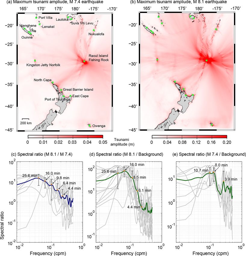
Y. Wang et al.: Characteristics of two tsunamis generated by successive M w 7.4 and M w 8.1 earthquakes 1075
(Figs. 1 and S1 in the Supplement) as a reference to confirm rectangular dimension of 240 km (length) × 190 km (width)
the findings obtained with tide gauges. with strike and dip angles of 210 and 16◦ , respectively.
The spatial intervals of sub-faults are 10 km × 10 km. We
2.2 Spectral analyses used Okada’s dislocation model (Okada, 1985) to compute
the seafloor deformation and used it as the initial condition
Two types of spectral analyses were conducted to tide gauge for tsunami propagation modeling. The bathymetric grids
records: Fourier analysis and wavelet (frequency–time) anal- were obtained from the General Bathymetric Chart of the
ysis. For Fourier analysis, a Hanning window with 40 % Oceans and resampled to 0.9 arcmin. The JAGURS numer-
overlaps was applied following the method of Heidarzadeh ical package (Baba et al., 2015) was adopted to simulate the
and Mulia (2021). The tsunami generated by the foreshock tsunami propagation based on linear long-wave equations.
(hereafter, the first tsunami) was clearly recorded at eight The time step for numerical simulations is 1.0 s. We simu-
tide gauges: North Cape (NC); Great Barrier Island (GBI); lated two tsunamis separately up to 12 h after the earthquake
East Cape (EC); Suva, Viti Levu (SVL); Lenakel; Quinne; origin time. Tsunami travel time (TTT) calculation was per-
Kingston Jetty, Norfolk (KJN); and Raoul Island Fishing formed for the second tsunami by the TTT software of Ge-
Rock (RIFR). However, it is difficult to accurately distin- oware (2011).
guish the arrival times at these stations. We used the 2 h seg-
ment before the arrival of the second tsunami as the input 2.4 Calculating tsunami source period
for spectral analyses. For RIFR, we utilized the 2 h segment
before the time it lost connection. The second tsunami gen- In this study, we calculated tsunami source period from finite
erated by the mainshock was clearly recorded at all the tide fault models to compare with the results of spectral analyses.
gauges except for RIFR. We selected a 2 h time segment af- Theoretically, the tsunami source period is related to earth-
ter the tsunami arrival as the input for Fourier analysis. Ad- quake rupture length and water depth (Rabinovich, 1997,
ditionally, background spectra were calculated using the 2 h 2010; Heidarzadeh and Satake, 2013; Wang et al., 2021). It
records before the arrival time of the first tsunami at the same can be estimated as
stations. We ensured that there were no storms or other at- 2L
mospheric events at the time period of the background sig- Tn = √ n = 1, 2, 3, . . ., (1)
n gh
nals, so the background spectra could exclusively reflect the
frequency response of local topography (Cortés et al., 2017; where L is the typical size of tsunami source area (length
Aránguiz et al., 2019). Tidal components were removed by or width), g is the gravity acceleration, and h is the average
applying a high-pass filter in a similar way to preparation of water depth in source area.
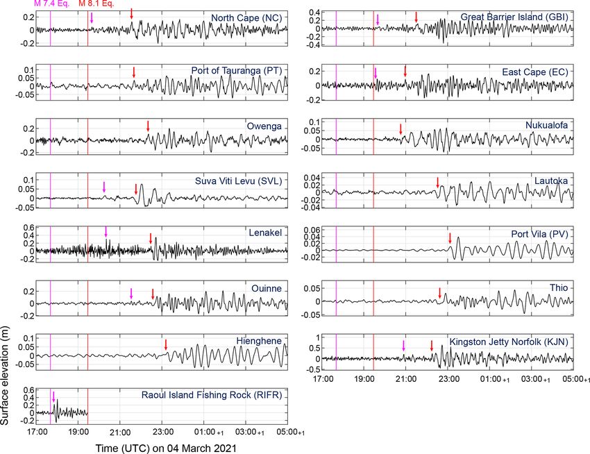
the tsunami records (Heidarzadeh and Satake, 2013).
Wavelet analysis was adopted to study the temporal
changes of the dominant spectral peaks and the superposi- 3 Tsunami waveform analysis
tion of two tsunamis. We applied the wavelet package pro-
vided by Torrence and Compo (1998), which uses the Morlet Two tsunamis arrive successively at 15 tide gauges (Fig. 2).
wavelet mother function. We only conducted wavelet analy- The first tsunami arrived at the RIFR station 11 min after
sis to seven tide gauges that clearly recorded both tsunamis. the foreshock. The first peak and the maximum amplitudes
The waveform segments for wavelet analyses are the same as are 0.21 and 0.34 m, respectively. It reached EC at 117 min
those used for Fourier analyses. after the earthquake with a maximum amplitude of 0.09 m.
It is noteworthy that the Lenakel tide gauge, located in the
2.3 Earthquake slip models and tsunami numerical direction parallel to the short axis of the earthquake source
simulation fault, recorded a maximum amplitude of 0.31 m. It is the
largest value among all stations except for the RIFR. The first
We used numerical simulation to study the propagation paths tsunami was also recorded by KJN with a maximum ampli-
of the two tsunamis. For the initial condition, the finite fault tude of 0.21 m.
models provided by the USGS were adopted (slip model The arrival times of the second tsunami are generally
of the first event at https://earthquake.usgs.gov/earthquakes/ consistent with the results of the TTT calculations (Fig. 1;
eventpage/us7000dfk3/finite-fault, last access: 4 June 2021; dashed contours) with clear large amplitude signals. It ar-
slip model of the second event at https://earthquake.usgs.gov/ rived at EC at 20:59 UTC; 91 min after the mainshock with
earthquakes/eventpage/us7000dflf/finite-fault, last access: an amplitude of 0.09 m. Yet the maximum amplitude at
4 June 2021). The source model of the first (Mw 7.4) earth- this station (0.17 m) appeared in a later time (approximately
quake has a rectangular dimension of 80 km (length) × 80 km 1 h after the first arrival) (Fig. 2). The largest waves were
(width). The strike and dip angles are 196 and 32◦ , respec- also observed at a later time in other stations such as NC,
tively. The spatial intervals of sub-faults are 4 km × 4 km. GBI, Nukualofa, Owenga, Ouinne, and Hienghene (Fig. 2).
The source model of the second (Mw 8.1) earthquake has a Such a late arrival of largest tsunami wave was reported
https://doi.org/10.5194/nhess-22-1073-2022 Nat. Hazards Earth Syst. Sci., 22, 1073–1082, 2022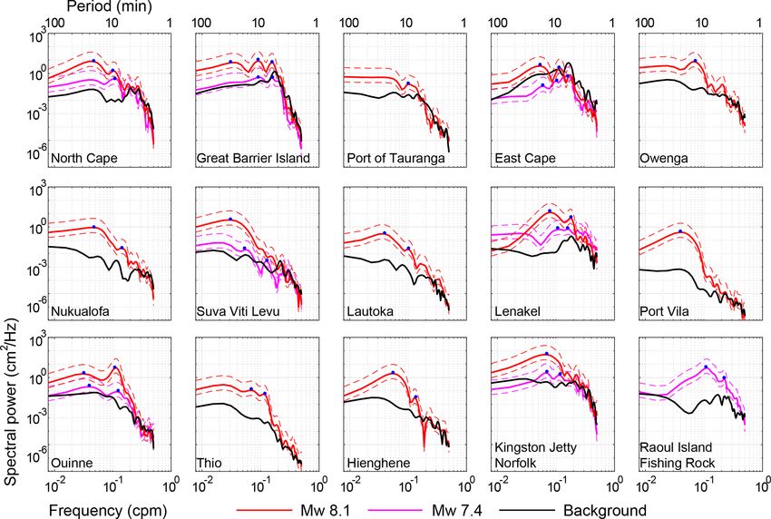
1076            Y. Wang et al.: Characteristics of two tsunamis generated by successive M w 7.4 and M w 8.1 earthquakes

Figure 2. Sea level change recorded by tide gauges showing two tsunamis. The pink and red vertical lines show the origin times of the
Mw 7.4 and Mw 8.1 earthquakes, respectively. The arrival times of the first and second tsunamis are marked by pink and red arrows, respec-
tively.

for other tsunamis in the past such as for the 2004 Indian             after the second tsunami’s arrival, but the waveforms af-
Ocean tsunami (Rabinovich and Thomson, 2007) and the                   ter 01:00 UTC (+1) were dominated by long-period compo-
2020 Aegean Sea tsunami (Heidarzadeh et al., 2021). The                nents (Fig. 2).
largest tsunami amplitude (0.64 m) was recorded by KJN,
which is also located in the direction parallel to the short
axis of the fault. Besides, the second tsunami has a longer            4   Spectral analyses
wavelength than the first tsunami, leading to longer tsunami
periods. At stations without a clear signal of the first tsunami       Figure 3 presents the results of Fourier analyses for two
(e.g., Lautoka), the tsunami waveforms are dominant by the             tsunamis and background signals. The gap between the
long-period components which are generated by the sec-                 tsunami and background spectra is attributed to the tsunami
ond tsunami. However, the stations that recorded both events           energy. The periods of the tsunami spectral peaks generally
show the superposition of two successive tsunamis. For ex-             contain the effects of tsunami source, propagation path, and
ample, the waveform of the second tsunami at EC is mixed               local topography. According to Fig. 3, the second tsunami
up with the short-period components in the few hours af-               has larger energy (spectral power) than the first tsunami due
ter its arrival (21:00–24:00 UTC), likely caused by the os-            to the larger magnitude of the second earthquake. The back-
cillation of the first tsunami (Fig. 2). After 24:00 UTC, the          ground spectra are smoother than tsunami spectra at most
tsunami waveforms mainly present long-period components,               stations. The peak periods of the first tsunami are mostly dis-
possibly due to the dissipation of the short-period waves              tributed in the range of 5–17 min, whereas the dominant pe-
of the first tsunami. Similar patterns were also observed at           riod range for the second tsunami is approximately 8–32 min.
Ouinne: short-period components existed in the few hours               In other words, the second tsunami generated longer-period

Nat. Hazards Earth Syst. Sci., 22, 1073–1082, 2022                                      https://doi.org/10.5194/nhess-22-1073-2022
Y. Wang et al.: Characteristics of two tsunamis generated by successive M w 7.4 and M w 8.1 earthquakes                                          1077

Figure 3. Fourier analyses for tsunamis generated by two successive earthquakes (Mw 7.4 and Mw 8.1) in the Kermadec Islands. Pink and
red curves represent the spectra of the first tsunami and the second tsunami, respectively. Blue dots show the spectral peaks listed in Table 1.
The 95 % confidence bounds of two tsunami spectra are indicated by dashed curves. The background spectra (black curves) are also plotted
for comparison.

waves, which is natural as the source dimension of the second
earthquake (240 km × 190 km) is much larger than that of the              Table 1. Peak periods at each tide gauge for two tsunami events.
first earthquake (80 km × 80 km). In Fig. S1, we plotted the              The values were calculated by Fourier analyses. Station name ab-
Fourier spectra of DART stations NZG and NZI. The spec-                   breviations are North Cape (NC), Great Barrier Island (GBI), East
tral peaks of these stations were generally consistent with               Cape (EC), Suva Viti Levu (SVL), Kingston Jetty Norfolk (KJN),
those of tide gauges. Regarding the tsunami-dominant period               Port Vila (PV), and Raoul Island Fishing Rock (RIFR).
(or peak periods), here we chose the period range that more
than half of the stations present as the dominant range. In Ta-               Tide gauge         Peak period(s) for the       Peak period(s) for the
ble 1, we listed the peak periods at each tide gauge for the                                        first tsunami (min)       second tsunami (min)
two tsunamis. Tsunami spectra can help identify the source                    NC                                        9.1                9.8; 21.3
size, potential asperities, and other information about earth-                GBI                                 6.5; 10.7          6.4; 10.7; 32.0
quake source processes. The dominant wave period ranges                       PT                                        n/a                      9.8
for tsunami events are related to the size of the source, which               EC                             6.1; 9.8; 16.0                8.5; 18.3
we explain in Sect. 5. Assuming the same water depths,                        Owenga                                    n/a                     14.2
tsunamis generated by earthquakes with larger source sizes                    Nukualofa                                 n/a                7.1; 21.3
normally have longer dominant wave periods. For example,                      SVL                                 8.0; 18.3                     32.0
the tsunami generated by the Mw 9.1 2004 Sumatra earth-                       Lautoka                                   n/a                9.8; 25.6
                                                                              Lenakel                              6.1; 8.5                5.6; 12.8
quake in the near-field region indicated dominance of long
                                                                              PV                                        n/a                     25.6
waves with periods of 30–60 min (Rabinovich et al., 2006).
                                                                              Ouinne                              8.5; 25.6                9.1; 32.0
   Wavelet analyses reveal the variations of dominant                         Thio                                      n/a                8.5; 14.2
tsunami frequency over time (Fig. 4). At EC, Lenakel, and                     Hienghene                                 n/a                7.5; 18.3
KJN, the arrivals of two successive tsunamis can be clearly                   KJN                                 8.5; 14.2                     14.2
identified on the wavelet plots. The second tsunami has larger                RIFR                                 4.6; 9.1                      n/a
energy levels and longer-period waves than the first tsunami
                                                                            n/a stands for not applicable.
(Fig. 4), which is consistent with the results of Fourier anal-
yses. At other stations such as GBI, the arrival time of the

https://doi.org/10.5194/nhess-22-1073-2022                                          Nat. Hazards Earth Syst. Sci., 22, 1073–1082, 2022
1078 Y. Wang et al.: Characteristics of two tsunamis generated by successive M w 7.4 and M w 8.1 earthquakes Figure 4. Wavelet (frequency–time) analyses for tsunamis generated by two successive earthquakes (Mw 7.4 and Mw 8.1) in the Kermadec Islands. The colormap shows levels of spectral energy at different times and periods. For guidance, we marked the dominant periods of two tsunamis by pink (Mw 7.4) and red (Mw 8.1) rectangles. The pink and red vertical lines show the origin times of the Mw 7.4 and Mw 8.1 earthquakes, respectively. The dispersion curves are plotted by black dashed lines. On the horizontal axis, plus one (+1) indicates one day passed. first tsunami is not clear. At most tide gauges, there are two tsunami. The oscillation lasts for more than 5 h. It is notewor- oscillation patterns visible on the wavelet plots. One oscilla- thy that after the arrival of the second tsunami, the oscillation tion pattern has dominant periods in the range of 5–17 min. pattern with short dominant periods still exists and becomes The other one has dominant periods over 15 min and up even stronger sometimes, indicating the contribution of both to approximately 30 min, which occurs after the first pat- tsunamis at EC. Two oscillation patterns simultaneously ex- tern. These two period bands on the wavelet plots reflect the ist for several hours and almost simultaneously diminish. The first and the second tsunamis. For example, the wavelet plot wavelet plot of KJN shows similar patterns to that of EC. Al- of EC reveals a persisting wave in the period range of 5– though there are also two oscillation patterns on the wavelet 11 min. The oscillation begins at approximately 2 h after the plot of Lenakel, the long-period oscillation only lasts for less Mw 7.4 earthquake, which corresponds to the arrival time of than 5 h. To the contrary, at GBI, the oscillation pattern with the first tsunami. Another oscillation with longer dominant long dominant periods lasts for approximately 3 h, whereas periods begins at approximately 2 h after the Mw 8.1 earth- the oscillation pattern with short dominant periods lasts for quake, which is consistent with the arrival time of the second more than 6 h. At Ouinne, a persisting wave in the period Nat. Hazards Earth Syst. Sci., 22, 1073–1082, 2022 https://doi.org/10.5194/nhess-22-1073-2022
Y. Wang et al.: Characteristics of two tsunamis generated by successive M w 7.4 and M w 8.1 earthquakes                     1079

band of 20–30 min is visible with high energy. Another oscil-     ized average. The period range of main energy (7–28 min)
lation pattern (6–12 min) diminishes earlier, which explains      contains spectral peaks at 25.6, 16.0, and 8.5 min, which are
the reason why the tsunami waveforms at Ouinne have fewer         close to the spectral peaks calculated by EGF method. In ad-
short-period components in the later phases (Fig. 2). Never-      dition, we also computed the spectral ratio of the first tsunami
theless, different from other stations, we cannot find a long-    to the background signals at those tide gauges with evident
lasting wave at SVL. There is only one oscillation period         records and calculated their normalized average (Fig. 5e).
band (20–40 min) and it diminishes rapidly. We note that the      This plot yields only the dominant periods of the first tsunami
dispersive effects of tsunamis from the second event are ev-      (generated by Mw 7.4 earthquake) showing that the energy is
ident on the wavelet plots as the tsunami-dominant period         mainly distributed in the period range of 5–17 min, indicat-
for the few initial waves is around ∼ 20 min, whereas it lin-     ing that the size of the tsunami source of the first event is
early shifts towards ∼ 10 min for the later waves, giving us      smaller than that of the second event.
the opportunity to plot the inverse dispersion lines (black          According to the USGS model, the size of the
dashed lines in Fig. 4). We plotted the dispersion curve on       Mw 8.1 earthquake is 240 km (length of the fault) × 190 km
these diagrams. We also observe short-period waves with a         (width of the fault). However, the non-zero displacement re-
period of 5–8 min at some sea-level stations (Table 1; Figs. 3    gion is approximately 210 km × 170 km (https://earthquake.
and 4), which we attribute to various local bathymetric ef-       usgs.gov/earthquakes/eventpage/us7000dflf/finite-fault, last
fects. In addition, we also note that wavelet and Fourier anal-   access: 4 June 2021). The average water depth in the source
yses give spectral results with varying degrees of accuracies,    area is ∼ 5000 m. Hence, the first three source periods of the
because wavelet analysis also incorporates the time evolu-        short axis of the source (width) using the analytical equation
tion and thus its spectra are not usually as detailed as those    (Eq. 1) are calculated as 25.6, 12.8, and 8.5 min. These values
obtained by Fourier analyses.                                     are consistent with the results of spectral analyses of the ob-
                                                                  served waves based on the EGF and tsunami-to-background
                                                                  spectral ratio methods (Fig. 5c and d) showing peak peri-
5   Reconstructing the tsunami source spectrum                    ods at 25.6, 16.0, and 9.8 min (8.5 min). We acknowledge
                                                                  that Eq. (1) is a rough approximation of dominant tsunami
A tsunami source spectrum reveals the earthquake source           source periods, and therefore we allowed a discrepancy of up
characteristics without the effects of tsunami propagation        to 20 % while making the comparison. We note that the peri-
path or local topography. In our study, the epicenters of         ods of tsunami waves are mainly influenced by the short axis
two earthquakes are close to each other (∼ 55 km; Fig. 1);        (width) (Heidarzadeh and Satake, 2013).
the earthquakes are of similar mechanism (both thrust                In addition, the results of two methods (i.e., EGF and
events). We simulated the propagation of two tsunamis us-         tsunami-to-background spectral ratio) show similarities in
ing JAGURS code and plotted their maximum amplitude in            shapes and peak periods of tsunami source spectrum (Fig. 5c
our region of interest to investigate their propagation path      and d). It is noted that the EGF method has the capability
(Fig. 5a and b). The tsunami amplitude in the NW–SE di-           to remove both propagation-path effects and local bathymet-
rection is larger than that in the NE–SW direction because        ric effects from the tide gauge records, whereas the tsunami-
it is parallel to the short axis of the fault. The propagation    to-background spectral ratio method would remove mainly
paths of two successive tsunamis are similar. Hence, it en-       local bathymetric effects. Hence, our results may imply that
ables us to reconstruct tsunami source spectrum using the         the effects of propagation path are negligibly small for this
EGF method which assumes that the smaller event acts as           case, where the tide gauges are located at distances between
the EGF for the larger event (Miller, 1972; Heidarzadeh et        ∼ 100 and ∼ 2000 km from the source. Both of the methods
al., 2016). We computed the spectral ratio of the second          are able to reveal the source characteristics merely based on
tsunami to the first tsunami at seven tide gauges (Fig. 5c;       tsunami observations rather than seismological data.
gray curves) and then calculated their normalized average            As limitations of this study, we could mention a few items:
values (Fig. 5c; blue curve) by adjusting the peak energy of      we are not using DART data (Fig. S1) to compute tsunami
all spectra to that of the largest one. The source spectrum       source spectrum due to the short duration of high-sampling
shows that the energy of the second tsunami is mainly dis-        records. In general, DART records are a valuable type of sea
tributed in the period range of 8–30 min, with spectral peaks     level data in terms of tsunami source studies because they are
at 25.6, 16.0, and 9.8 min. The period range is generally con-    less affected by local and regional bathymetry. In addition,
sistent with the results of Fourier analyses of each station      the number of sea level records that we used for analyses of
for the second event (Fig. 3). Figure 5d shows the results of     these tsunamis is not very large due to the limited number of
the method proposed by Rabinovich (1997) which is based           available stations.
on dividing the tsunami spectra to that of the background to
construct tsunami source spectrum. We computed the spec-
tral ratio of the second tsunami to the background signals
at all tide gauges except RIFR and calculated their normal-

https://doi.org/10.5194/nhess-22-1073-2022                               Nat. Hazards Earth Syst. Sci., 22, 1073–1082, 2022
1080 Y. Wang et al.: Characteristics of two tsunamis generated by successive M w 7.4 and M w 8.1 earthquakes
Figure 5. (a, b) Maximum simulated amplitudes for two tsunamis during the entire simulation time. The source models used for numerical
simulation are from the USGS. (c) Spectral ratio of two tsunamis by dividing the spectral energy of the second tsunami to that of the first
tsunami (EGF method). Blue curve is the normalized average of tsunami spectral energy at different tide gauges. (d) Spectral ratio of the
second tsunami spectrum to the background signal spectrum. Green curve is the normalized average of different tide gauges. (e) Spectral
ratio of the first tsunami spectrum to the background signal spectrum. Green curve is the normalized average of different tide gauges.
6 Conclusion ond tsunami, the oscillation in the period range of the first
tsunami still exists. We calculated the tsunami source spec-
We studied the characteristics of the tsunamis generated by trum of the larger event (i.e., the second tsunami) with two
two earthquakes (Mw 7.4 and Mw 8.1) that occurred in the approaches: empirical Green’s function (EGF) method and
Kermadec Islands successively on 4 March 2021, within tsunami-to-background ratio method. Using the first tsunami
∼ 55 km from each other and within an approximately 2 h as the EGF, spectral deconvolution indicated that energy of
interval. We used the sea level records of 15 tide gauges. the second tsunami is mainly distributed in the period range
The spectra of Fourier analyses show that the dominant of 8–30 min, with spectral peaks at 25.6, 16.0, and 9.8 min.
period bands of the first tsunami and the second tsunami The method of tsunami-to-background ratio yielded simi-
are 5–17 and 8–32 min, respectively. Two oscillation pat- lar results to the EGF method. The source characteristics
terns with different period ranges are visible on the wavelet were obtained merely based on tsunami data, and thus these
plots at most stations which belong to the first and the sec- two methods could be complementary to seismological ap-
ond tsunamis. We observed that after the arrival of the sec- proaches in source analysis.
Nat. Hazards Earth Syst. Sci., 22, 1073–1082, 2022 https://doi.org/10.5194/nhess-22-1073-2022Y. Wang et al.: Characteristics of two tsunamis generated by successive M w 7.4 and M w 8.1 earthquakes 1081
Data availability. The datasets were derived from sources in References
the public domain. The tide gauge data used in this research
were provided by the Sea Level Station Monitoring Facility of Aránguiz, R., Catalán, P. A., Cecioni, C., Bellotti, G., Hen-
the Intergovernmental Oceanographic Commission (http://www. riquez, P., and González, J.: Tsunami resonance and
ioc-sealevelmonitoring.org/list.php; IOC, 2022). We used bathy- spatial pattern of natural oscillation modes with multi-
metric and topographic data of the General Bathymetric Chart ple resonators, J. Geophys. Res.-Oceans, 124, 7797–7816,
of the Ocean (https://www.gebco.net/data_and_products/gridded_ https://doi.org/10.1029/2019JC015206, 2019.
bathymetry_data/; GEBCO, 2022). We used the earthquake fo- Baba, T., Takahashi, N. Kaneda, Y. Ando, K. Matsuoka,
cal mechanism catalog of the Global Centroid Moment Tensor D., and Kato, T.: Parallel implementation of dispersive
Project (https://www.globalcmt.org/CMTsearch.html; Global CMT, tsunami wave modeling with a nesting algorithm for the
2022) and the earthquake source model of the United States Geo- 2011 Tohoku Tsunami, Pure Appl. Geophys., 172, 3433–3472,
logical Survey (https://earthquake.usgs.gov/earthquakes/eventpage/ https://doi.org/10.1007/s00024-015-1049-2, 2015.
us7000dflf/executive; USGS, 2022). We used the GMT software for Billen, M. I., Gurnis, M., and Simons, M.: Multiscale dynamics
drafting some of the figures (Wessel and Smith, 1998). of the Tonga-Kermadec subduction zone, Geophys. J. Int., 153,
359–388, https://doi.org/10.1046/j.1365-246X.2003.01915.x,
2003.
Supplement. The supplement related to this article is available on- Cortés, P., Catalán, P. A., Aránguiz, R., and Bellotti,
line at: https://doi.org/10.5194/nhess-22-1073-2022-supplement. G.: Tsunami and shelf resonance on the northern
Chile coast, J. Geophys. Res.-Oceans, 122, 7364–7379,
https://doi.org/10.1002/2017JC012922, 2017.
GEBCO: Global ocean & land terrain models, GEBCO [code],
Author contributions. YW was responsible for the methodology,
https://www.gebco.net/data_and_products/gridded_bathymetry_
data curation, software, and writing (original draft preparation).
data/, last access: 29 March 2022.
MH was responsible for the methodology, software, and writing (re-
Geoware: The Tsunami Travel Times (TTT) Package, http://www.
viewing and editing). KS was responsible for methodology, super-
geoware-online.com/tsunami.html (last access: 1 August 2021),
vision, and writing (reviewing and editing). GH was responsible for
2011.
data curation and software.
Global CMT: CMT Catalog Citation Information, https://www.
globalcmt.org/CMTsearch.html, last access: 29 March 2022.
Heidarzadeh, M., and Mulia, I. E.: Ultra-long period and small-
Competing interests. The contact author has declared that neither amplitude tsunami generated following the July 2020 Alaska
they nor their co-authors have any competing interests. Mw 7.8 tsunamigenic earthquake, Ocean Eng., 234, 109243,
https://doi.org/10.1016/j.oceaneng.2021.109243, 2021.
Heidarzadeh, M. and Satake, K.: Waveform and spectral analyses of
Disclaimer. Publisher’s note: Copernicus Publications remains the 2011 Japan tsunami records on tide gauge and DART stations
neutral with regard to jurisdictional claims in published maps and across the Pacific Ocean, Pure Appl. Geophys., 170, 1275–1293,
institutional affiliations. https://doi.org/10.1007/s00024-012-0558-5, 2013.
Heidarzadeh, M. and Satake, K.: New insights into the source of the
Makran tsunami of 27 November 1945 from tsunami waveforms
Special issue statement. This article is part of the special issue and coastal deformation data, Pure Appl. Geophys., 172, 621–
“Tsunamis: from source processes to coastal hazard and warning”. 640, https://doi.org/10.1007/s00024-014-0948-y, 2015.
It is not associated with a conference. Heidarzadeh, M., Satake, K., Murotani, S., Gusman, A. R.,
and Watada, S.: Deep-Water Characteristics of the Trans-
Pacific Tsunami from the 1 April 2014 Mw 8.2 Iquique,
Acknowledgements. We thank Takane Hori and Kentaro Imai from Chile Earthquake, Pure Appl. Geophys., 172, 719–730,
the Japan Agency for Marine-Earth Science Technology for their https://doi.org/10.1007/s00024-014-0983-8, 2015.
valuable suggestions. Mohammad Heidarzadeh is funded by the Heidarzadeh, M., Harada, T., Satake, K., Ishibe, T., and Gusman,
Royal Society (the United Kingdom), grant no. CHL\R1\180173. A. R.: Comparative study of two tsunamigenic earthquakes in
Yuchen Wang is funded by the Japan Society for the Promotion of the Solomon Islands: 2015 Mw 7.0 normal-fault and 2013 Santa
Science, grant no. 19J20293. Cruz Mw 8.0 megathrust earthquakes, Geophys. Res. Lett., 43,
4340–4349, https://doi.org/10.1002/2016GL068601, 2016.
Heidarzadeh, M., Pranantyo, I. R., Okuwaki, R., Dogan, G. G.,
Financial support. This research has been supported by the Japan and Yalciner, A. C.: Long tsunami oscillations following the
Society for the Promotion of Science (grant no. 19J20293) and the 30 October 2020 Mw 7.0 Aegean Sea earthquake: Observa-
Royal Society (grant no. CHL\R1\180173). tions and modelling, Pure Appl. Geophys., 178, 1531–1548,
https://doi.org/10.1007/s00024-021-02761-8, 2021.
IOC: Sea Level Station Monitoring Facility, IOC [data set],
http://www.ioc-sealevelmonitoring.org/list.php, last access:
Review statement. This paper was edited by Fabrizio Romano and
29 March 2022.
reviewed by Alexander Rabinovich and two anonymous referees.
Lundgren, P. R., Okal, E. A., and Wiens, D. A.: Rup-
ture characteristics of the 1982 Tonga and 1986 Ker-
https://doi.org/10.5194/nhess-22-1073-2022 Nat. Hazards Earth Syst. Sci., 22, 1073–1082, 20221082 Y. Wang et al.: Characteristics of two tsunamis generated by successive M w 7.4 and M w 8.1 earthquakes madec earthquakes, J. Geophys. Res.-Solid, 94, 15521–15539, Romano, F., Gusman, A. R., Power, W., Piatanesi, A., Volpe, https://doi.org/10.1029/JB094iB11p15521, 1989. M., Scala, A., and Lorito, S.: Tsunami Source of the Miller, G. R.: Relative spectra of tsunamis, HIG-72-8, incl. Table 2021 Mw 8.1 Raoul Island Earthquake from DART and Tide- and Figs., Hawaii Inst. Geophys., Honolulu, 17 pp., 1972. Gauge Data Inversion, Geophys. Res. Lett., 48, e2021GL094449, Morgan, P. G.: The New Zealand earthquake of August 6, 1917, https://doi.org/10.1029/2021GL094449, 2021. Bull. Seismol. Soc. Am., 8, 127–128, 1918. Torrence, C. and Compo, G.: A practical guide to wavelet analysis, Okada, Y.: Surface deformation due to shear and tensile faults in a B. Am. Meteorol. Soc., 79, 61–78, https://doi.org/10.1175/1520- half-space, Bull. Seismol. Soc. Am., 75, 1135–1154, 1985. 0477(1998)0792.0.CO;2, 1998. Power, W., Wallace, L., Wang, X., and Reyner, M.: Tsunami USGS: M 8.1 – Kermadec Islands, New Zealand, USGS Hazard Posed to New Zealand by the Kermadec and South- [data set], https://earthquake.usgs.gov/earthquakes/eventpage/ ern New Hebrides Subduction Margins: An Assessment us7000dflf/executive, last access: 29 March 2022. Based on Plate Boundary Kinematics, Interseismic Coupling, Wang, Y., Zamora, N., Quiroz, M., Satake, K., and Cienfue- and Historical Seismicity, Pure Appl. Geophys., 169, 1–36, gos, R.: Tsunami resonance characterization in Japan due https://doi.org/10.1007/s00024-011-0299-x, 2012. to trans-Pacific sources: Response on the bay and conti- Rabinovich, A. B.: Spectral analysis of tsunami waves: Separation nental shelf, J. Geophys. Res.-Oceans, 126, e2020JC017037, of source and topography effects, J. Geophys. Res.-Oceans, 102, https://doi.org/10.1029/2020JC017037, 2021. 12663–12676, https://doi.org/10.1029/97JC00479, 1997. Wessel, P. and Smith, W. H. F.: New, improved version of Rabinovich, A. B.: Seiches and harbor oscillations, generic mapping tools released, Eos Trans. AGU, 79, 579, in: Handbook of coastal and ocean engineering, https://doi.org/10.1029/98EO00426, 1998. World Scientific Publishing, Singapore, 193–236, Wyss, M., Habermann, R. E., and Griesser, J.-C.: https://doi.org/10.1142/9789812819307_0009, 2010. Seismic quiescence and asperities in the Tonga- Rabinovich, A. B. and Thomson, R. E.: The 26 December 2004 Kermadec Arc, J. Geophys. Res.-Solid, 89, 9293–9304, Sumatra tsunami: Analysis of tide gauge data from the world https://doi.org/10.1029/JB089iB11p09293, 1984. ocean Part 1. Indian Ocean and South Africa, Pure Appl. Geo- phys., 164, 261–308, https://doi.org/10.1007/978-3-7643-8364- 0_2, 2007. Rabinovich, A. B., Thomson, R. E., and Stephenson, F.: The Suma- tra tsunami of 26 December 2004 as observed in the North Pa- cific and North Atlantic oceans, Surv. Geophys., 27, 647–677, https://doi.org/10.1007/s10712-006-9000-9, 2006. Nat. Hazards Earth Syst. Sci., 22, 1073–1082, 2022 https://doi.org/10.5194/nhess-22-1073-2022
You can also read