Changes in black carbon emissions over Europe due to COVID-19 lockdowns
←
→
Page content transcription
If your browser does not render page correctly, please read the page content below
Atmos. Chem. Phys., 21, 2675–2692, 2021
https://doi.org/10.5194/acp-21-2675-2021
© Author(s) 2021. This work is distributed under
the Creative Commons Attribution 4.0 License.

Changes in black carbon emissions over Europe due to
COVID-19 lockdowns
Nikolaos Evangeliou1 , Stephen M. Platt1 , Sabine Eckhardt1 , Cathrine Lund Myhre1 , Paolo Laj2,3,4 ,
Lucas Alados-Arboledas5,6 , John Backman7 , Benjamin T. Brem8 , Markus Fiebig1 , Harald Flentje9 ,
Angela Marinoni10 , Marco Pandolfi11 , Jesus Yus-Dìez11 , Natalia Prats12 , Jean P. Putaud13 , Karine Sellegri14 ,
Mar Sorribas15 , Konstantinos Eleftheriadis16 , Stergios Vratolis16 , Alfred Wiedensohler17 , and Andreas Stohl18
1 Department    of Atmospheric and Climate Research (ATMOS), Norwegian Institute for Air Research (NILU), Kjeller, Norway
2 University  of Grenoble Alpes, CNRS, IRD, Grenoble-INP, IGE, 38000 Grenoble, France
3 CNR-ISAC, National Research Council of Italy – Institute of Atmospheric Sciences and Climate, Bologna, Italy
4 Atmospheric Science division, University of Helsinki, Helsinki, Finland
5 Department of Applied Physics, Andalusian Institute for Earth System Research (IISTA-CEAMA), Granada, Spain
6 Department of Applied Physics, University of Granada, Granada, Spain
7 Atmospheric Composition Research, Finnish Meteorological Institute, Helsinki, Finland
8 Laboratory of Atmospheric Chemistry, Paul Scherrer Institute, Villigen PSI, Switzerland
9 Deutscher Wetterdienst, Meteorologisches Observatorium Hohenpeissenberg, Albin-Schwaiger-Weg 10,

82383 Hohenpeissenberg, Germany
10 National Research Council of Italy (ISAC-CNR), Institute of Atmospheric Sciences and Climate, 40121, Bologna, Italy
11 Institute of Environmental Assessment and Water Research IDAEA-CSIC, C/Jordi Girona 18–26,

Barcelona 08034, Spain
12 Izaña Atmospheric Research Center, State Meteorological Agency (AEMET), C/La Marina 20, 38001, Tenerife, Spain
13 European Commission, Joint Research Centre (JRC), Via Enrico Fermi 2749, Ispra (VA) 21027, Italy
14 Laboratoire de Météorologie Physique, UMR6016, CNRS/UBP, 63178 Aubière, France
15 El Arenosillo Atmospheric Sounding Station, Atmospheric Research and Instrumentation Branch, National Institute for

Aerospace Technology, 21130 Huelva, Spain
16 Environmental Radioactivity Lab, Institute of Nuclear & Radiological Sciences & Technology, Energy & Safety, NCSR

“Demokritos”, Ag. Paraskevi, Athens, Greece
17 Department Experimental Aerosol and Cloud Microphysics, Leibniz Institute for Tropospheric Research, Leipzig, Germany
18 Department of Meteorology and Geophysics, University of Vienna, UZA II, Althanstraße 14, 1090 Vienna, Austria

Correspondence: Nikolaos Evangeliou (nikolaos.evangeliou@nilu.no)

Received: 26 September 2020 – Discussion started: 5 October 2020
Revised: 17 January 2021 – Accepted: 18 January 2021 – Published: 23 February 2021

Abstract. Following the emergence of the severe acute res-       which strict lockdowns were applied, due to lower pollutant
piratory syndrome coronavirus 2 (SARS-CoV-2) responsible         emissions. Here we investigate the effects of the COVID-19
for COVID-19 in December 2019 in Wuhan (China) and its           lockdowns in Europe on ambient black carbon (BC), which
spread to the rest of the world, the World Health Organization   affects climate and damages health, using in situ observations
declared a global pandemic in March 2020. Without effec-         from 17 European stations in a Bayesian inversion frame-
tive treatment in the initial pandemic phase, social distanc-    work. BC emissions declined by 23 kt in Europe (20 % in
ing and mandatory quarantines were introduced as the only        Italy, 40 % in Germany, 34 % in Spain, 22 % in France) dur-
available preventative measure. In contrast to the detrimen-     ing lockdowns compared to the same period in the previ-
tal societal impacts, air quality improved in all countries in   ous 5 years, which is partially attributed to COVID-19 mea-

Published by Copernicus Publications on behalf of the European Geosciences Union.
2676                                 N. Evangeliou et al.: Changes in black carbon emissions due to COVID-19 lockdowns

sures. BC temporal variation in the countries enduring the         tems and climate with the global economy (Diffenbaugh et
most drastic restrictions showed the most distinct lockdown        al., 2020).
impacts. Increased particle light absorption in the beginning         Strongly light absorbing black carbon (BC, or “soot”), is
of the lockdown, confirmed by assimilated satellite and re-        produced from incomplete combustion of carbonaceous fu-
mote sensing data, suggests residential combustion was the         els, e.g. fossil fuels, wood-burning and biofuels (Bond et
dominant BC source. Accordingly, in central and Eastern Eu-        al., 2013). By absorbing solar radiation, it warms the air
rope, which experienced lower than average temperatures,           and reduces tropical cloudiness (Ackerman, 2000) and at-
BC was elevated compared to the previous 5 years. Never-           mospheric visibility (Jinhuan and Liquan, 2000). BC causes
theless, an average decrease of 11 % was seen for the whole        pulmonary diseases (Wang et al., 2014a), may act as cloud
of Europe compared to the start of the lockdown period, with       condensation nuclei, affecting cloud formation and precipi-
the highest peaks in France (42 %), Germany (21 %), UK             tation (Wang et al., 2016), and contributes to global warming
(13 %), Spain (11 %) and Italy (8 %). Such a decrease was          (Bond et al., 2013; Myhre et al., 2013; Wang et al., 2014a).
not seen in the previous years, which also confirms the im-        When deposited on snow, it reduces snow albedo (Clarke and
pact of COVID-19 on the European emissions of BC.                  Noone, 1985; Hegg et al., 2009), accelerating melting. Since
                                                                   BC is both climate-relevant and strongly linked to anthro-
                                                                   pogenic activity, it is important to determine the effects of
                                                                   the COVID-19 lockdowns thereon.
                                                                      Here, we present a rigorous assessment of temporal and
1   Introduction                                                   spatial changes BC emissions over Europe (including the
                                                                   Middle East and parts of North Africa), combining in situ
The identification of the severe acute respiratory syndrome        observations from the Aerosol, Clouds and Trace Gases Re-
coronavirus 2 (SARS-CoV-2 or COVID-19) in Decem-                   search Infrastructure (ACTRIS) network and state-of-the-art
ber 2019 (WHO, 2020) in Wuhan (China) and its subse-               emission inventories within a Bayesian inversion. We vali-
quent transmission to South Korea, Japan and Europe (ini-          date our results with independent satellite data and compare
tially mainly Italy, France and Spain) and the rest of the         them to inventories’ baseline and optimized emissions calcu-
world led the World Health Organization to declare a global        lated for previous years.
pandemic by March 2020 (Sohrabi et al., 2020). Although the
symptoms are normally mild or not even detected for most
of the population, people with underlying diseases or the el-      2   Methods
derly are very vulnerable, showing complications that can
lead to death (Huang et al., 2020). Considering the lack of        This section gives a detailed description of all datasets and
available treatment and vaccination to combat further spread       methods used for the calculation of COVID-19 impact. Sec-
of the virus, the only prevention measures included strict         tion 2.1 describes the instrumentation of the particle light
social, travel and working restrictions in a so-called lock-       absorption measurements from Aerosol, Clouds and Trace
down period that lasted for several weeks (mid-March to end        Gases Research Infrastructure (ACTRIS) and the networks
of April 2020 for most of Europe). The most drastic mea-           European Monitoring and Evaluation Program (EMEP) and
sures were taken in China, where the outbreak started, in          Global Atmosphere Watch (GAW). These measurements
Italy that faced large human losses and later in the United        were used in the inverse modelling algorithm (dependent
States. Despite all these restrictions, still 6 months after the   measurements) and to validate the optimized (posterior)
first lockdown, several countries are reporting severe hu-         emissions of BC (independent measurements). For each of
man losses due to the virus (John Hopkins University of            the observations and stations, the source–receptor matrices
Medicine, 2020).                                                   (SRMs), also known as “footprint emission sensitivities” or
   Despite the dramatic health and socioeconomic conse-            “footprints”, were calculated as described in Sect. 2.2. The
quences of COVID-19 lockdowns, their environmental im-             latter together with the observations were fed into the inver-
pact might be beneficial. Bans on mass gatherings, manda-          sion algorithm described in Sect. 2.3. To overcome classic
tory school closures and home confinement (He et al., 2020;        inverse problems (Tarantola, 2005), prior (a priori) emissions
Le Quéré et al., 2020) during lockdowns have all resulted          of BC were used in the inverse modelling algorithm, calcu-
in lower traffic-related pollutant emissions and improved          lated using bottom-up approaches (Sect. 2.4). The optimized
air quality in Asia, Europe and America (Adams, 2020;              (a posteriori) emissions of BC were compared with reanaly-
Bauwens et al., 2020; Berman and Ebisu, 2020; Conticini et         sis data from MERRA-2 (Modern-Era Retrospective Analy-
al., 2020; Dantas et al., 2020; Dutheil et al., 2020; He et al.,   sis for Research and Applications Version 2), which are de-
2020; Kerimray et al., 2020; Le et al., 2020; Lian et al., 2020;   scribed in Sect. 2.5, while MERRA-2 Ångström exponent
Otmani et al., 2020; Sicard et al., 2020; Zheng et al., 2020).     data, together with the absorption Ångström exponent from
The restrictions also present an opportunity to evaluate the       the Aerosol Robotic Network (AERONET) (Sect. 2.6), were
cascading responses from the interaction of humans, ecosys-        used to examine the presence of biomass burning aerosols in

Atmos. Chem. Phys., 21, 2675–2692, 2021                                             https://doi.org/10.5194/acp-21-2675-2021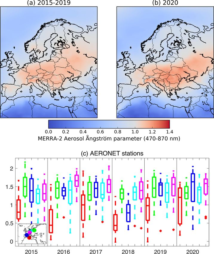
N. Evangeliou et al.: Changes in black carbon emissions due to COVID-19 lockdowns                                           2677

Europe. A description of the statistical tests and the country    FLEXPART also simulates dry and wet deposition (Grythe
definitions used in the paper is given in Sect. 2.7 and 2.8,      et al., 2017), turbulence (Cassiani et al., 2014) and unre-
respectively.                                                     solved mesoscale motions (Stohl et al., 2005) and includes
                                                                  a deep convection scheme (Forster et al., 2007). SRMs were
2.1   Particle light absorption measurements                      calculated for 30 d backward in time, at temporal intervals
                                                                  that matched measurements at each receptor site. This back-
The measurement sites contributing data to this paper are         ward tracking is sufficiently long to include almost all BC
regional background sites (except for one site in Germany)        sources that contribute to surface concentrations at the re-
and all contribute to the research infrastructure ACTRIS and      ceptors given a typical atmospheric lifetime of 3–11 d (Bond
the networks EMEP and GAW. The measurement data used              et al., 2013).
for the period 2015–May 2020 consist of hourly averaged,
quality-checked, particle light absorption measurements. The      2.3   Bayesian inverse modelling
quality assurance and quality control correspond to the Level
2 requirements for ACTRIS, EMEP and GAW data, as de-              The Bayesian inversion framework FLEXINVERT+ de-
scribed in detail in Laj et al. (2020).                           scribed in detail in Thompson and Stohl (2014) was used
   All absorption measurements within ACTRIS and EMEP             to optimize emissions of BC before (January to mid-
are taken using a variety of filter-based photometers: Multi-     March 2020) and during the COVID-19 lockdown period in
Angle Absorption Photometer (MAAP), Particle Soot Ab-             Europe (mid-March to end of April 2020). To show potential
sorption Photometer (PSAP) Continuous Light Absorption            differences in the signal from the 2020 restrictions, emissions
Photometer (CLAP) and the Aethalometer (AE-31). Infor-            were optimized with the same setup during the same period
mation on instrument type at the various sites is included        (January to April) in the previous 5 years (2015–2019). Note
in Table 1, and procedures for harmonization of measure-          that the number of stations in the inversions of 2015–2019
ment protocols to produce comparable datasets are described       was slightly higher (20 stations against 15 that were used in
in Laj et al. (2020) in detail. Zanatta et al. (2016) sug-        2020), due to different data availability. The algorithm finds
gested that a mass absorption cross-section (MAC) value of        the optimal emissions which lead to FLEXPART-modelled
10 m2 g−1 (geometric standard deviation of 1.33) at a wave-       concentrations that better match the observations consider-
length of 637 nm can be considered to be representative of        ing the uncertainties for observations, prior emissions and
the mixed boundary layer at European ACTRIS background            SRMs. Specifically, the state vector of BC concentrations,
sites, where BC is expected to be internally mixed to a large       mod , at M points in space and time can be modelled given
                                                                  y(M×1)
extent. Assuming an absorption Ångström exponent (AAE)            an estimate of the emissions, x (N×1) , of the N state variables
is equal to unity, i.e. assuming no change in MAC for differ-     discretized in space and time, while atmospheric transport
ent sources (Zotter et al., 2017), we extrapolated the MACs       and deposition are linear operations described by the Jaco-
at 637 nm (MAC@λ1 ) to the measurement wavelengths of our         bian matrix of SRMs, H(M×N) :
study (MAC@λ2 ) using the following equation:
                                                                  y mod = H x + ,                                            (2)
                 λ1
MAC@λ2 = MAC@λ1 ( )AAE
                 λ2                                               where  is an error associated with model representation,
           yields           637 1                                 such as the modelled transport and deposition or the mea-
          −−−→ MAC@λ2 = 10(    ) ,                         (1)    surements. Since H is not invertible or may not have a unique
                            λ2
                                                                  inverse, according to Bayesian statistics, the inverse problem
following Lack and Langridge (2013). The resulting MAC            can be described as the maximization of the probability den-
values for each measurement station are shown in Table 1.         sity function of the emissions given the prior information and
                                                                  observations. This is equivalent to the minimum of the cost
2.2   Source–receptor matrix (SRM) calculations                   function:
SRMs for each of the 17 receptor sites (Table 1) were calcu-             1
lated using the Lagrangian particle dispersion model FLEX-        J (x) = (x − x b )T B−1 (x − x b )
                                                                         2
PART version 10.4 (Pisso et al., 2019). The model releases               1
computational particles that are tracked backward in time               + (y − Hx)T R−1 (y − Hx),                             (3)
                                                                         2
based on 3-hourly operational meteorological analyses from
the European Centre for Medium-Range Weather Forecasts            where y is the vector of observed BC concentrations, and
(ECMWF) with 137 vertical layers and a horizontal resolu-         x and x b are the vectors of optimized and prior emissions,
tion of 1◦ × 1◦ . The tracking of BC particles includes gravi-    respectively, while B and R are the error covariance ma-
tational settling for spherical particles, with an aerosol mean   trices that weight the posterior–prior flux and observation–
diameter of 0.25 µm, a logarithmic standard deviation of 0.3      model mismatches, respectively. Based on Bayes’ theorem,
and a particle density of 1500 kg m−3 (Long et al., 2013).        the most probable posterior emissions, x, are given by the

https://doi.org/10.5194/acp-21-2675-2021                                             Atmos. Chem. Phys., 21, 2675–2692, 2021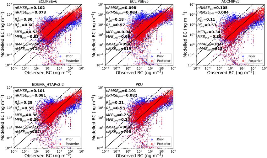
2678                                  N. Evangeliou et al.: Changes in black carbon emissions due to COVID-19 lockdowns

Table 1. Observation sites from the ACTRIS platform used to perform the inversions (dependent observations) and to validate the posterior
emissions (independent observations) (the altitude indicates the sampling height in metres above sea level). A Multi-Angle Absorption
Photometer (MAAP) was used at all sites, except El Arenosillo (ES0100R), where a Continuous Light Absorption Photometer (CLAP) was
used, Birkenes (NO0002R), where a Particle Soot Absorption Photometer (PSAP) was used and Observatoire Perenne de l’Environnement
(FR0022R) and Zeppelin (NO0042G), where an Aethalometer (AW-31) was used.

               Name                      Latitude    Longitude    Altitude   Type               Wavelength     MAC@637
                                                                                                      (nm)      (m2 g−1 )
               Jungfraujoch                 46.55         7.99       3578    Dependent                  637            10
               (CH0001G)
               Hohenpeissenberg             47.80        11.01        985    Dependent                  660          9.65
               (DE0043G)
               Melpitz                      51.53        12.93         86    Dependent                  670          8.78
               (DE0044K)
               Zugspitze-                   47.42        10.98       2671    Independent                670          9.51
               Schneefernerhaus
               (DE0054R)
               Leipzig-                     51.35        12.41        120    Independent                670          9.51
               Eisenbahnstrasse
               (DE0066K)
               Izaña (ES0018G)              28.41      −16.50        2373    Dependent                  670          9.51
               Granada                      37.16       −3.61         680    Dependent                  670          9.51
               (ES0020U)
               Montsec                      42.05         0.73       1571    Dependent                  670          9.51
               (ES0022R)
               El Arenosillo                37.10       −6.73          41    Dependent                  652         13.64
               (ES0100R)
               Montseny                     41.77         2.35        700    Dependent                  670          8.48
               (ES1778R)
               Pallas                       67.97        24.12        565    Dependent                  637         10.00
               (FI0096G)
               Observatoire                 48.56         5.51        392    Dependent                  880          7.24
               Perenne de
               l’Environnement
               (FR0022R)
               Puy de Dôme                  45.77         2.96       1465    Dependent                  670          9.51
               (FR0030R)
               Ispra                        45.80         8.63        209    Dependent                  880          6.96
               (IT0004R)
               Mt Cimone                    44.18        10.70       2165    Dependent                  670          9.51
               (IT0009R)
               Birkenes II                  58.39         8.25        219    Dependent                  660          7.59
               (NO0002R)
               Zeppelin mountain            78.91        11.89        474    Dependent                  880          7.24
               (NO0042G)

Atmos. Chem. Phys., 21, 2675–2692, 2021                                                  https://doi.org/10.5194/acp-21-2675-2021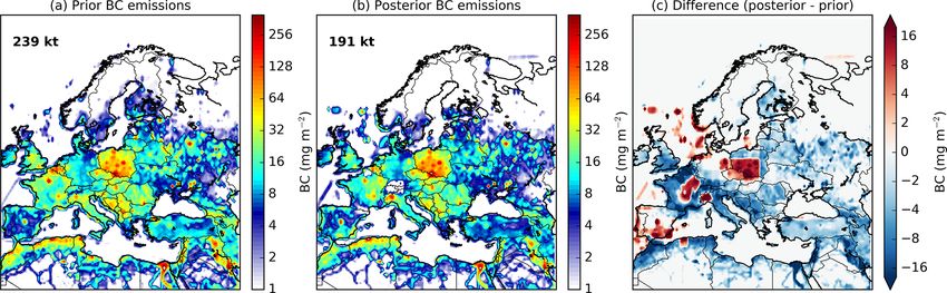
N. Evangeliou et al.: Changes in black carbon emissions due to COVID-19 lockdowns 2679
similarly using the time difference between grid cells in dif-
ferent time steps. The full temporal and spatial correlation
matrix is given by the Kronecker product (see Thompson and
Stohl, 2014). The error covariance matrix for the emissions
is the matrix product of correlation pattern and the error co-
variance of the prior fluxes. We calculate the error on the
emissions in each grid cell (on the fine grid) as a fraction of
the maximum value out of that grid cell and the eight sur-
rounding ones.
The observation error covariance matrix R combines mea-
surement, transport model and representation errors. For
the measurement errors, we use values given by the data
providers. Transport model errors are difficult to quantify and
depend not only on the model but also on the meteorological
inputs. Therefore, we do not quantify the full transport er-
ror but only the part of it that can be estimated from FLEX-
PART, i.e. the stochastic uncertainty (see Stohl et al., 2005).
As regards to representation errors, we consider observation
representation error and model aggregation error. The obser-
vation representation error is calculated from the standard
deviation of all measurements available in a user-specified
measurement averaging time interval, based on the idea that
if the measurements are fluctuating strongly within that in-
terval, then their mean value is associated with higher un-
certainty than if the measurements are steady (Bergamaschi
et al., 2010). The aggregation error is attributed to reduction
of the spatial resolution of the model and is calculated by
projecting the loss of information in the state space into the
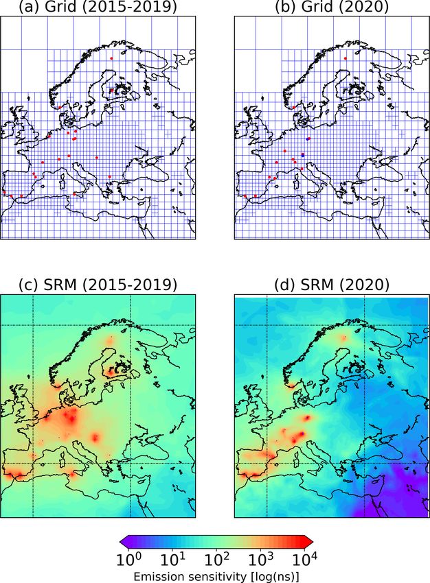
Figure 1. Aggregated inversion grid used for the (a) 2015–2019 and observation space (Kaminski et al., 2001). Hence, the obser-
(b) 2020 inversions, respectively. The dependent measurements that vation error covariance matrix is defined as the diagonal ma-
were used in the inversion were taken from stations highlighted in
trix with elements equal to the quadratic sum of the mea-
red. The two independent stations that were used for the validation
are shown in blue. (c, d) Footprint emission sensitivity (i.e. SRM)
surement, transport model and measurement representation
averaged over all observations and time steps for each of the inver- errors (Thompson and Stohl, 2014).
sions. Red points denote the location of each measurement site. Theoretically, the algorithm can calculate negative poste-
rior emissions, which are physically unlikely. To tackle this
problem, an inequality constraint was applied on the emis-
following equation (Tarantola, 2005): sions following the method of Thacker (2007) that applies
−1 the constraint as “error-free” observations:
x = x b + BHT HBHT + R (y − Hx b ). (4) −1
x̂ = x + APT PAPT (c − Px), (5)
Here, posterior emissions were calculated weekly between
1 January and 30 April 2020. The aggregated inversion grid where A is the posterior error covariance matrix, P is a ma-
(25–75◦ N and 10◦ W–50◦ E) and the average SRM for in- trix operator to select the variables that violate the inequality
versions are shown in Fig. 1, while the measurement stations constraint and c is a vector of the inequality constraint, which
are listed in Table 1. The variable grid uses high resolution in in this case is zero.
regions in which there are many stations and hence strong We evaluated the assumptions made on the error covari-
contribution from emissions, while it lowers resolution in ance matrices for the prior emissions and the observations
regions that lack measurement stations, following a method using the reduced χ 2 statistics (B and R). When χ 2 is equal
proposed by Stohl et al. (2010). to unity, the posterior solution is within the limits of the pre-
Prior emission errors B are correlated in space and time, scribed uncertainties. The latter is the value of the cost func-
but very little is known about the true temporal and spatial er- tion at the optimum (Thompson et al., 2015). In the inver-
ror correlation patterns. The spatial error correlation for the sions performed here, the calculated χ 2 values were between
emissions is defined as an exponential decay over distance 0.8 and 1.5, indicating that the chosen uncertainty parame-
(we assume that emissions on land and ocean are not cor- ters are close to the ideal ones. The number of measurements
related). The temporal error correlation matrix is described used in each inversion was equal to 12 538 from 17 stations.
https://doi.org/10.5194/acp-21-2675-2021 Atmos. Chem. Phys., 21, 2675–2692, 2021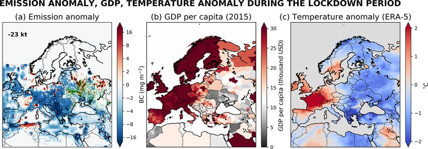
2680                                 N. Evangeliou et al.: Changes in black carbon emissions due to COVID-19 lockdowns

To select the inversion that provides the most statistically sig-   MERRA-2 are simulated with the Goddard Chemistry,
nificant result, an evaluation of the improvement in the poste-     Aerosol, Radiation and Transport (GOCART) model and
rior modelled concentrations, with respect to the prior ones,       delivered in hourly to monthly temporal resolution and at
against the observations was performed (Fig. 2). The result-        0.5◦ × 0.625◦ spatial resolution. The product has been val-
ing values of each of the statistical measures that were per-       idated for AOD, PM and BC extensively (Buchard et al.,
formed are given in detail in Table 2. Note that this is not        2017; Qin et al., 2019; Randles et al., 2017; Sun et al., 2019).
a validation of the posterior emissions because the compar-         The Ångström exponent (AE), a measure of how the AOD
ison is only done for the observations that were included in        changes relative to the various wavelength of light, is derived
the inversion (dependent observations), and the inversion al-       here from AOD469, AOD550, AOD670 and AOD865, by fit-
gorithm has been designed to reduce the model–observation           ting the data to the linear transform of Ångström’s empirical
mismatches. This means that the reduction of the posterior          expression:
concentration mismatches to the observations is determined
by the weighting that is given to the observations with re-                      λ −a
                                                                    τλ = τλ0 (      ) ,                                           (6)
spect to the prior emissions. A proper validation of the pos-                    λ0
terior emissions is performed against observations that were
not included in the inversion (independent observations) in         where τλ is the known AOD at wavelength λ (in nm), τλ0 is
Sect. 3.3.                                                          the AOD at 1000 nm and α stands for AE (Gueymard and
                                                                    Yang, 2020).
2.4    Prior emissions
                                                                    2.6     Absorption Ångström exponent from Aerosol
As a priori emissions in the inversions, the ECLIPSE version                Robotic Network (AERONET) data
5 and 6 (Evaluating the CLimate and Air Quality ImPacts
of ShortlivEd Pollutants) (Klimont et al., 2017), EDGAR             Aerosol composition over Europe during the COVID-19
(Emissions Database for Global Atmospheric Research) ver-           lockdown was confirmed using the AERONET data (Holben
sion HTAP_v2.2 (Janssens-Maenhout et al., 2015), ACCMIP             et al., 1998). AERONET provides globally distributed ob-
(Emissions for Atmospheric Chemistry and Climate Model              servations of spectral aerosol optical depth (AOD), inversion
Intercomparison Project) version 5 (Lamarque et al., 2013)          products and precipitable water in diverse aerosol regimes.
and PKU (Peking University) (Wang et al., 2014b) were               The AE for a spectral dependence of 440–870 nm is related to
used (Fig. 3). All inventories include the basic emission sec-      the aerosol particle size. Values less than 1 suggest an optical
tors (e.g. waste burning, industrial combustion and process-        dominance of coarse particles corresponding to dust, ash and
ing, all means of transportation (aerial, surface, ocean), en-      sea spray aerosols, while values greater than 1 imply domi-
ergy conversion and residential and commercial combustion;          nance of fine particles such as smoke and industrial pollution
see references therein). Biomass burning emissions were             (Eck et al., 1999). We chose data from five stations cover-
adopted from the Global Fire Emissions Database, Version            ing Western, central and Eastern Europe, for which cloud-
4.1s (GFEDv4.1s) (Giglio et al., 2013). Note that the a priori      free measurements exist for the lockdown period, namely
emissions used in the inversions of 2015–2019 period corre-         Ben Salem (9.91◦ E, 35.55◦ N), Minsk (27.60◦ E, 53.92◦ N),
sponded to year 2015 of ECLIPSEv6, and they were not in-            Montsec (0.73◦ E, 42.05◦ N), MetObs Lindenberg (14.12◦ E,
terpolated for the years between 2015 and 2020, for which           52.21◦ N) and Munich University (11.57◦ E, 48.15◦ N). We
the ECLIPSEv6 emissions were calculated. We calculate               used Level 1.5 absorption AE (AAE) measurements for the
that the anthropogenic emissions of BC in Europe between            COVID-19 lockdown period (14 March to 30 April 2020).
January–April 2015 and January–April 2020 in ECLIPSEv6
                                                                    2.7     Statistical measures
differ by 3.4 % only, and therefore we expected that this
would not add significant bias in our calculations.
                                                                    For the performance evaluation of the inversion results
                                                                    against dependent (observations that were included in the
2.5    MERRA-2 (Modern-Era Retrospective Analysis for
                                                                    inversion) and independent observations (observations that
       Research and Applications Version 2)
                                                                    were not included in the inversion), four different statistical
                                                                    quantities were used.
The MERRA-2 reanalysis dataset for BC (Randles et
al., 2017) assimilates bias-corrected aerosol optical depth           1. Pearson’s correlation coefficient was calculated as fol-
(AOD) from Moderate Resolution Imaging Spectrora-                        lows:
diometer (MODIS), Advanced Very High Resolution Ra-
diometer (AVHRR) instruments, Multiangle Imaging Spec-                                      n
                                                                                                Pn
                                                                                                 mi oi − ni=1 mi ni=1 oi
                                                                                                        P       P
                                                                                             i=1
troRadiometer (MISR) and Aerosol Robotic Network                          Rmo = q P                       q P                        ,
                                                                                 n ni=1 m2i − ( ni=1 mi )2 n ni=1 oi2 − ( ni=1 oi )2
                                                                                               P                         P
(AERONET) with the Goddard Earth Observing System
Model Version 5 (GEOS-5). BC and other aerosols in                                                                                (7)

Atmos. Chem. Phys., 21, 2675–2692, 2021                                                   https://doi.org/10.5194/acp-21-2675-2021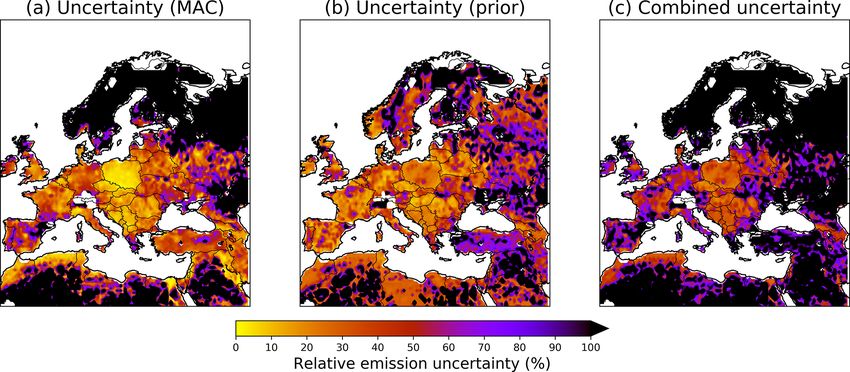
N. Evangeliou et al.: Changes in black carbon emissions due to COVID-19 lockdowns                                                   2681

Figure 2. Scatter plots of prior and posterior concentrations against dependent observations (observations that were included in the in-
version framework) from ACTRIS from January to April 2020. Four statistical measures (nRMSE, Pearson’s R 2 , MFB and nMAE) were
used to assess the performance of each inversion using five different prior emission inventories for BC (ECLIPSEv5, v6, ACCMIPv5,
EDGAR_HTAPv2.2 and PKU).

Table 2. Statistical measures (RMSE, Pearson’s R 2 , MFB and nMAE) for each of the prior and posterior concentrations against dependent
observations (observations that were used in the inversion algorithm) for BC (eBC). Note that the inversion using ECLIPSEv6 prior emission
dataset gave the best agreement with the observations, and therefore the results of this inversion are presented here.

                                                               nRMSE      Pearson’s R 2     MFB     nMAE
                              Prior ECLIPSEv6                   0.102          0.30         0.52       997
                              Prior ECLIPSEv5                   0.098          0.18        −0.04       996
                              Prior EDGAR_HTAPv2.2              0.105          0.11         0.34      1017
                              Prior ACCMIPv5                    0.101          0.28         0.36       971
                              Prior PKU                         0.101          0.21         0.25       983
                              Posterior ECLIPSEv6               0.073          0.60         0.03       714
                              Posterior ECLIPSEv5               0.084          0.52         0.09       819
                              Posterior EDGAR_HTAPv2.2          0.084          0.53         0.20       815
                              Posterior ACCMIPv5                0.091          0.55         0.26       787
                              Posterior PKU                     0.082          0.55         0.24       795

     where n is the sample size, m and o the individual sam-             2. The normalized root mean square error (nRMSE) was
     ple points for model concentrations and observations in-               calculated as follows:
     dexed with i.                                                                      qP
                                                                                             n 1             2
                                                                                             i=1 n (mi − oi )
                                                                            nRMSE =                            .           (8)
                                                                                            oimax − oimin

                                                                         3. The mean fractional bias (MFB) was selected as a sym-
                                                                            metric performance indicator that gives equal weights

https://doi.org/10.5194/acp-21-2675-2021                                                  Atmos. Chem. Phys., 21, 2675–2692, 2021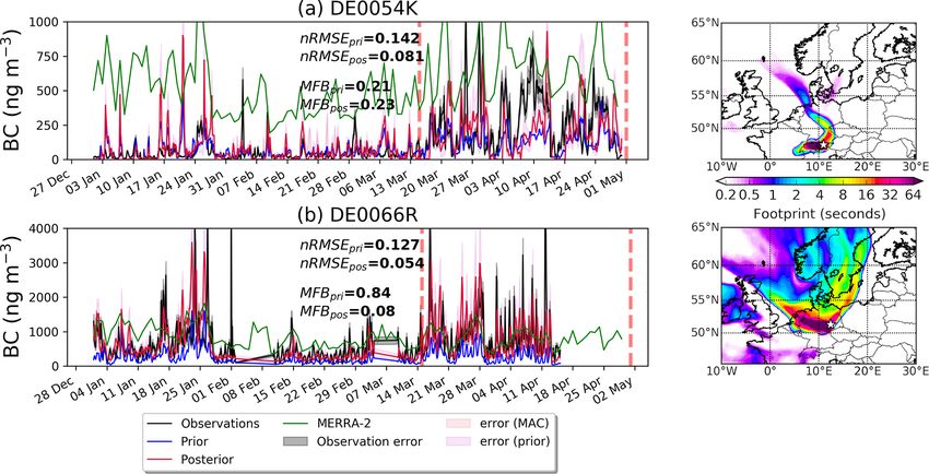
2682                                 N. Evangeliou et al.: Changes in black carbon emissions due to COVID-19 lockdowns

Figure 3. Prior emissions of black carbon (BC) used in the inversions. BC emissions from anthropogenic sources were adopted from
ECLIPSE version 5 and 6 (Evaluating the CLimate and Air Quality ImPacts of ShortlivEd Pollutants) (Klimont et al., 2017), EDGAR
(Emissions Database for Global Atmospheric Research) version HTAP_v2.2 (Janssens-Maenhout et al., 2015), ACCMIP (Emissions for
Atmospheric Chemistry and Climate Model Intercomparison Project) version 5 (Lamarque et al., 2013) and PKU (Peking University) (Wang
et al., 2014b). Biomass burning emissions of BC from Global Fire Emissions Database (GFED) version 4.1 (Giglio et al., 2013) were added
to each of the aforementioned inventories.

      to under- or overestimated concentrations (minimum to           Europe is defined by France, Belgium, Holland, Germany,
      maximum values range from −200 % to 200 %) and is               Austria and Switzerland. Eastern Europe includes Poland,
      defined as                                                      Czechia, Slovakia, Hungary, Romania, Bulgaria, Moldova,
               1 ni=1 (mi − oi )
                 P                                                    Ukraine, Belarus and Russia.
      MFB =       Pn mi +oi .                           (9)
               n    i=1 ( 2 )
                                                                      3     Results
  4. The mean absolute error was computed normalized
     (nMAE) over the average of all the actual values (obser-         3.1    Optimized (posterior) emissions from Bayesian
     vations here), which is a widely used simple measure of                 inversion
     error:
               Pn
                     |mi − oi |                                       We performed five inversions for BC over Europe for
     nMAE = i=1     Pn          .                        (10)         1 January–30 April 2020, each with different prior emis-
                     i=1 oi                                           sions from ECLIPSE version 5 and 6, EDGAR version
2.8    Region definitions                                             HTAP_v2.2, ACCMIP version 5 and PKU (Fig. 3). Total
                                                                      prior emissions of BC in Europe from the five emission in-
All country and regional masks are publicly available. Re-            ventories for the period of the inversion ranged between 192–
gions used for statistical processing purposes were adopted           377 kt. We evaluated the assumptions made on the error co-
from the United Nations Statistics Division (https://unstats.         variance matrices for the prior emissions and the observa-
un.org/home/, last access: 25 September 2020). Accordingly,           tions using the reduced χ 2 statistic (B and R; see Sect. 2.3).
Northern Europe includes UK, Norway, Denmark, Swe-                    When χ 2 is equal to unity, the posterior solution is within the
den, Finland, Iceland, Estonia, Latvia and Lithuania. South-          limits of the prescribed uncertainties. The performance of the
ern Europe includes Spain, Italy, Greece, Slovenia, Croa-             inversions with the five different prior inventories was evalu-
tia, Bosnia, Serbia, Albania and North Macedonia. Western             ated using four statistical parameters (see Sect. 2.7). The best

Atmos. Chem. Phys., 21, 2675–2692, 2021                                                 https://doi.org/10.5194/acp-21-2675-2021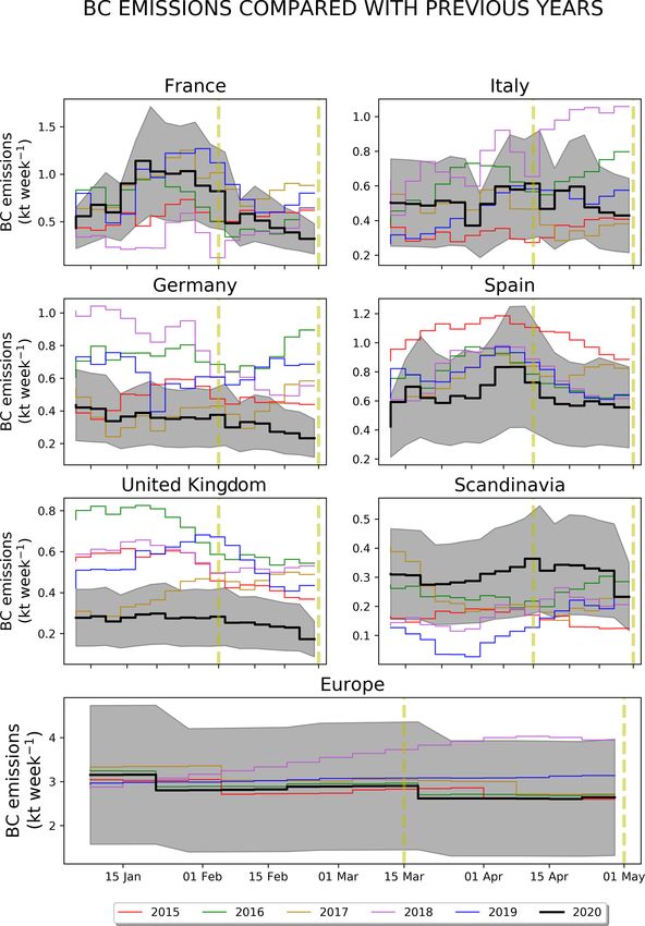
N. Evangeliou et al.: Changes in black carbon emissions due to COVID-19 lockdowns                                         2683

performance of the inversions was achieved using ECLIP-             Overall, BC emissions decreased by ∼ 46 kt during the
SEv6 (Table 2 and Fig. 2) with the smallest nRMSE (0.073)        COVID-19 lockdown in the inversion domain (10◦ W–50◦ E,
value, the largest Pearson’s R 2 (0.60), the MFB value closest   25–70◦ N) as compared with the same period in the previous
to zero (0.03) and the smallest nMAE (714). Therefore, all       5 years. We record a significant decrease in BC emissions in
the results presented below correspond to this inversion.        central Europe (northern Italy, Austria, Germany, Spain and
   Posterior emissions of BC were calculated to be 191 kt        some Balkan countries) (Fig. 5). On average, emissions were
in the inversion domain (10◦ W–50◦ E, 25–75◦ N) or ap-           23 kt lower (63 to 40 kt) over Europe during the lockdown in
proximately 20 % smaller than those in ECLIPSEv6 (239 kt)        2020 than in the same period of 2015–2019 (Fig. 5). The de-
(Fig. 4). Note that these numbers refer to the whole inver-      crease has the same characteristics when compared to each
sion domain (not only Europe) and the whole study period         of previous years since 2015 (Fig. S1) based on measure-
(January–April 2020). The largest posterior differences were     ments of BC in similar regions to those used for the 2020
found in the eastern part of the domain (20–50◦ E, 45–55◦ N),    inversion. The countries that showed drastic reductions in
where emissions dropped from 35 to 29 kt. Emissions of BC        BC emissions during the lockdowns were those that suffered
in the western part of the inversion domain (10◦ W–20◦ E,        from the pandemic dramatically, with many human losses,
45–55◦ N) declined by almost 11 % (from 45 to 40 kt) com-        strict social distancing rules and consequently less transport.
pared to those in the north part (5◦ W–35◦ E, 55–70◦ N) that     Specifically, compared with the previous 5 years, the 2020
covers Scandinavian countries (from 8.7 to 6.4 kt). Finally,     emissions of BC during the lockdowns dropped by 20 % in
in the southern part (10◦ W–50◦ E, 35–45◦ N) of the domain       Italy (3.4 to 2.7 kt), 40 % in Germany (3.3 to 2.0 kt), 34 %
(Spain, Italy, Greece), the posterior emissions also decreased   in Spain (4.7 to 3.1 kt) and 22 % in France (3.5 to 2.7 kt)
by 21 % relative to the priors (from 61 to 48 kt). The largest   and remained the same or were slightly enhanced in Poland
country decreases were seen in France (from 14 to 8.2 kt),       (∼ 9.2 kt) and Scandinavia (∼ 1.2 kt). Air quality in Poland
Italy (from 8.0 to 5.9 kt), UK (from 4.4 to 3.1 kt) and Ger-     may not be Europe’s worst, but its emissions stand out for
many (from 4.5 to 4.1 kt). Surprisingly, BC emissions were       their large spatial spread. Poland’s air pollution stems from
slightly enhanced in Poland (from 21 to 23 kt) and in Spain      its use of cheap coal for home heating rather than cleaner
(from 6.3 to 7.5 kt). In general, inversion algorithms reduce    natural gas common in neighbouring countries. This causes
the mismatches between modelled concentrations and ob-           smoke particles to rise up to 3 times higher than European av-
servations by correcting emissions (Sect. 2.3). If decreased     erage levels in winter and early spring (Bertelsen and Math-
posterior emissions are calculated during the whole inver-       iesen, 2020). Overall, BC emissions during the 2020 lock-
sion period (before and during the lockdowns), impact from       downs in Western Europe declined by 32 % (8.8 to 6.0 kt),
the COVID-19 restrictions cannot be concluded, and, most         in Southern Europe by 42 % (17 to 9.9 kt) and in Northern
likely, the reduced emissions are due to errors in the prior     Europe by 29 % (5.4 to 3.8 kt) as compared to the 2015–
emissions. In the next section (Sect. 3.2), we demonstrate       2019 period. BC emissions in Eastern Europe were slightly
that this decrease was due to the COVID-19 lockdowns, by         increased during the 2020 lockdown as compared to the same
comparing posterior emissions with emissions from previous       period in the last 5 years (28 to 31 kt). The hotspot emissions
years, as well as with the respective emissions before and       in Eastern Europe coincide with the presence of active fires
during the lockdown measures.                                    as revealed from MODIS (Fig. 5a). Note that these numbers
                                                                 correspond to BC emissions during the COVID-19 lockdown
3.2   Comparison with previous years                             period only (mid-March–April 2020).
                                                                    Some localized areas of increased BC emissions exist in
We also performed inversions for 2015–2019 for the same          southern France, Belgium, northern Germany and Eastern
period as the 2020 lockdowns (January–April) using almost        Europe (Fig. 5), which are observed relative to almost every
the same measurement stations and keeping the same set-          year since 2015 (Fig. S1). While some hotspots in France
tings. The difference in BC emissions during the lockdown        cannot be easily explained, increased emissions in Eastern
in 2020 (14 March to 30 April) to the respective emissions       European countries are likely due to increased residential
during the same period in 2015–2019 (14 March to 30 April)       combustion, as people had to stay at home during the lock-
is shown in Fig. 5a (emission anomaly), together with the        down. The combination of the financial consequences of the
gross domestic product (GDP) (Kummu et al., 2020) in 5b          COVID-19 lockdown with the relatively low GDP per capita
and temperature anomaly from ERA-5 (Copernicus Climate           in these countries and the fact that from mid-March to end
Change Service (C3S), 2020) in 5c for the same period as the     of April 2020 surface temperatures in these countries were
emission anomaly. The difference in the 2020 emissions of        significantly lower than in previous years is suggestive of in-
BC during the lockdown from the respective emissions in the      creased emissions due to residential combustion. This source
same period in each of the previous years (2015–2019) is il-     is most important in Eastern Europe (Klimont et al., 2017).
lustrated in Fig. S1. As an independent source of information,   Although residential combustion can be performed for heat-
active fires from the MODIS satellite product MCD14DL            ing or cooking needs in poorer countries, it is also believed
(Giglio et al., 2003) are also shown in Fig. 5a and Fig. S1.     to provide a more natural type of warmth and a comfortable

https://doi.org/10.5194/acp-21-2675-2021                                          Atmos. Chem. Phys., 21, 2675–2692, 2021
2684 N. Evangeliou et al.: Changes in black carbon emissions due to COVID-19 lockdowns
Figure 4. (a) Prior emissions of BC from ECLIPSEv6, (b) optimized (posterior) BC emissions after processing the ACTRIS data into the
inversion algorithm and (c) difference between posterior and prior emissions. All the results correspond to the inversion yielding the best
results (Table 2 and Fig. 2).
Figure 5. (a) Difference in posterior BC emissions during the lockdown (14 March to 30 April 2020) in Europe from the respective emissions
during the same period in 2015–2019, (b) GDP from Kummu et al. (2020) and (c) temperature anomaly from ERA-5 (Copernicus Climate
Change Service (C3S), 2020) for the same period as the emission anomaly. The base GDP value below which a low income can be assumed
was set to USD 12 000. Active fires from MODIS are plotted together with the emission anomaly (green dots).
and relaxing environment. Hence, it should not be assumed posterior emissions drastically. The first is the use of dif-
as an emission source in countries with lower GDPs only, ferent prior emissions; to estimate this type of uncertainty,
especially as people spent more time at home. Moreover, we performed five inversions for January to April 2020 us-
the prevailing average temperatures over Europe during the ing each of the prior emission datasets (ECLIPSEv6 and
lockdown were below 15 ◦ C (Fig. S2), a temperature used v5, EDGAR_HTAPv2.2, ACCMIPv5 and PKU). The uncer-
as a basis temperature below which residential combustion tainty was calculated as the gridded standard deviation of
increases (Quayle and Diaz, 1980; Stohl et al., 2013). the posterior emissions resulting from the five inversions.
The second type of uncertainty concerns measurement of
3.3 Uncertainty and validation of the posterior BC, which is defined as a function of five properties (Pet-
emissions zold et al., 2013). However, as of today, no single instrument
exists that can measure all of these properties at the same
time. Hence, BC is not a single particle constituent, rather an
One of the basic problems when dealing with inverse mod-
operational definition depending on the measurement tech-
elling is that changing model, observational or prior uncer-
nique (Petzold et al., 2013). Here we use light absorption co-
tainties can have drastic impacts on posterior emissions. We
efficients (Petzold et al., 2013) converted to equivalent BC
addressed this issue by finding the optimal parameters, in or-
(eBC) using the mass absorption cross-section (MAC). The
der to have a reduced χ 2 statistic around unity (see Sect. 2.3).
MAC is instrument-specific and wavelength-dependent. The
However, there are two other sources of uncertainty that, al-
site-specific MAC values used to convert the filter-based light
though not linked with the inversion algorithm, could affect
Atmos. Chem. Phys., 21, 2675–2692, 2021 https://doi.org/10.5194/acp-21-2675-2021N. Evangeliou et al.: Changes in black carbon emissions due to COVID-19 lockdowns 2685 absorption to eBC can be seen in Table 1. It has been reported dustries in the North Sea (Fig. 4b). In all these regions, the that MAC values vary from 2–3 up to 20 m2 g−1 (Bond and footprint emissions’ sensitivities corresponding to the two in- Bergstrom, 2006). To estimate the uncertainty of the poste- dependent stations were the highest. rior fluxes associated with the variable MAC, we performed a sensitivity study for January to April 2020 using MAC val- ues of 5, 10 and 20 m2 g−1 at all stations, as well as variable 4 Discussion MAC values for each station (Table 1). Since these values are log-normally distributed, the uncertainty is calculated as the The improved air quality that Europe experienced during the geometric standard deviation. The impact of other sources lockdown was also evident from the assimilated MERRA- of uncertainty, such as those referring to scavenging coeffi- 2 satellite-based BC data. The latter are plotted in Fig. S3 cients, particle size and density that are used in the model has (left axis) for 2015–2020, together with the posterior emis- been studied before and is significantly smaller than that of sions calculated in the present study (right axis). For in- the sources of uncertainty that are considered here (Evange- stance, weekly average concentrations of BC over Europe liou et al., 2018; Grythe et al., 2017). in MERRA-2 (Fig. S3, bottom). Many of the ACTRIS sta- The posterior emissions are less sensitive to the use of tions reported increased light absorption at the beginning of different MACs than the use of different prior inventories the lockdown (e.g. Fig. 7); MERRA-2 data show the same (Fig. 6). The relative uncertainty due to different use of MAC patterns in France, Italy, UK and Spain and in all of Eu- values was up to 20 %–30 % in most of Europe and increases rope, in general. This can be explained by residential com- dramatically (∼ 100 %) far from the observations. The emis- bustion, considering that the surface temperature during the sion uncertainty of BC from the use of different priors was lockdown was lower than in previous years (Fig. 5). The lat- estimated to be up to 40 % in Europe and shows very sim- ter was confirmed by the MERRA-2 reanalysis Ångström ex- ilar characteristics (same hotspot regions and larger values ponent (AE) parameter at 470–870 nm, which shows higher where measurements are lacking). Overall, the combined un- values over central and Eastern Europe during the lock- certainty of BC emissions was ∼ 60 % in Europe. down in 2020 than in the same period of the previous years Validation of top-down emissions obtained by inversion (Fig. 8a, b). Larger AE values confirm the presence of wood- algorithms can be proper only if measurements that were not burning aerosols (Eck et al., 1999). The fact that during the included in the inversion are to be used (independent obser- COVID-19 lockdown, residential combustion was a signifi- vations). For this reason, we left observations from two sta- cant aerosol source in Europe, as compared to the previous tions (DE0054K and DE0066R; Table 1) out of the inversion. years, was also confirmed by real-time observations of ab- Due to the higher measurement station density in central Eu- sorption AE from the AERONET data at five selected sta- rope, we randomly selected two German stations, rather than tions over Europe (Fig. 8c). Measured absorption AE was from a country that is adjacent to regions that lack observa- higher during mid-March to April 2020 than in the same pe- tions. riod of the last 5 years. The prior, optimized and measured concentrations are Emissions of BC calculated with Bayesian inversion for shown in Fig. 7, together with MERRA-2 surface BC con- the lockdown period dropped substantially in most of the centrations at the same stations. The average footprint emis- countries that suffered from further spread of the virus and, sion sensitivities are also given for the period of the lock- accordingly, from strict lockdown measures, as compared down. At station DE0054K, prior emissions represent obser- to the respective emissions before the lockdowns (Fig. S3). vations very well until the beginning of the lockdown and Specifically, the decrease in France was as high as 42 %, then fail (Fig. 7). On the other hand, the posterior emis- 8 % in Italy, 21 % in Germany, 11 % in Spain and 13 % in sions represent the variant concentrations during the lock- the UK. Emissions also declined in Scandinavia by 5 %, al- down effectively and also manage to capture some concentra- though Sweden did not enforce a lockdown. Overall, a re- tion peaks, which is reflected by a lower nRMSE. Backward duction in BC emissions of about 11 % can be concluded for modelling showed that the enhanced concentrations originate Europe as a whole due to the lockdown. Stronger decreases from northern Germany and the Netherlands, where poste- in Eastern Europe were likely partly compensated for by in- rior emissions were increased compared with the prior ones creased residential combustion, resulting from the prevailing (Fig. 4). A similar pattern was seen at station DE0066K, al- low temperatures. though this station showed concentrations of up to 4 mg m−3 We report a 23 kt decrease in BC emissions in Europe dur- (Fig. 7). Again, the optimized emissions managed to repre- ing the lockdown that partially resulted from the COVID- sent the peaks at the end of January 2020 and at the begin- 19 outbreak, as compared to the same period in all previous ning of the lockdown, which is again reflected by nRMSE years since 2015, based on particle light absorption measure- values reduced by a factor of 2 and MFB close to zero as ments. We highlight these changes in BC emissions partially compared to the priors. The larger concentrations during the as a result of COVID-19 restrictions by plotting the tempo- lockdown result from increased emissions over eastern Ger- ral variability of the BC emissions in the 5 previous years many, Poland and the Netherlands, as well as from oil in- (2015–2019) for France, Italy, Germany, Spain, Scandinavia https://doi.org/10.5194/acp-21-2675-2021 Atmos. Chem. Phys., 21, 2675–2692, 2021
2686                                     N. Evangeliou et al.: Changes in black carbon emissions due to COVID-19 lockdowns

Figure 6. (a) Uncertainty of BC emissions due to the use of variable MAC values to convert from aerosol absorption to eBC concentrations
that are used by the inversion algorithm. (b) Uncertainty due to the use of five different prior emissions inventories for BC. (c) Combined
uncertainty.

Figure 7. Prior and posterior BC concentrations at (a) DE0054K and (b) DE0066R stations that were not included in the inversion are
compared with observations. The validation is done by calculating the nRMSEs and MFBs for the prior and posterior concentrations. The
uncertainty of the observations is also given, together with the posterior uncertainties in the concentrations calculated from the use of different
MAC and prior emissions. For comparison, we plot the concentrations from MERRA-2 at the same two stations. The vertical dashed lines
denote the period of the lockdown in most of Europe. In the right-hand panels of (a) and (b), the average footprint emission sensitivities are
given at each independent station for the period of the lockdown.

and Europe (Fig. 9). We record decreases in BC emissions                    2020 lockdowns were significantly lower than those of the
in France, Italy, Germany and Scandinavia in mid-March to                   same period in any of the previous years. Overall, emissions
April 2020, opposite to what was estimated for all years be-                declined by 20 % in Italy, 40 % in Germany, 34 % in Spain
tween 2015 and 2019, which is obviously due to COVID-19.                    and 22 % in France and remained the same and slightly en-
The UK and Spain showed a similar decrease in mid-March                     hanced in Scandinavia and Poland as compared to those of
to April 2020 emissions as in all previous years (2015–2019).               the last 5 years.
However, the estimated posterior BC emissions during the

Atmos. Chem. Phys., 21, 2675–2692, 2021                                                         https://doi.org/10.5194/acp-21-2675-2021
N. Evangeliou et al.: Changes in black carbon emissions due to COVID-19 lockdowns                                                2687

Figure 8. (a) Average total aerosol Ångström parameter (470–870 nm) over Europe (mid-March to April) in the 5 previous years (2015–
2019) and (b) in 2020 (lockdown). (c) AERONET Absorption AE in Ben Salem (9.91◦ E, 35.55◦ N; in red), Minsk (27.60◦ E, 53.92◦ N;
green), Montsec (0.73◦ E, 42.05◦ N; blue), MetObs Lindenberg (14.12◦ E, 52.21◦ N; magenta) and Munich University (11.57◦ E, 48.15◦ N)
during mid-March to April in all years since 2015.

5   Conclusions                                                      ductions were calculated for countries that suffered from the
                                                                     pandemic dramatically, such as Italy (3.4 to 2.7 kt), Germany
                                                                     (3.3 to 2.0 kt), Spain (4.7 to 3.1 kt) and France (3.5 to 2.7 kt).
The impact of the COVID-19 lockdowns over Europe on
                                                                     BC emissions in Western Europe during the 2020 lockdowns
the BC emissions, in response to the pandemic, was as-
                                                                     were decreased from 8.8 to 6.0 kt (32 %), in Southern Eu-
sessed in the present paper. Particle light absorption mea-
                                                                     rope from 17 to 9.9 kt (42 %) and in Northern Europe from
surements from 17 ACTRIS stations all around Europe were
                                                                     5.4 to 3.8 kt (29 %) as compared to the same period in the
rapidly gathered and cleaned to produce a high-quality prod-
                                                                     last 5 years. BC emissions were slightly enhanced in East-
uct. The latter was used in a well-established Bayesian inver-
                                                                     ern Europe (from 28 to 31 kt) and remained unchanged in
sion framework, and BC emissions were optimized over Eu-
                                                                     Scandinavia during the lockdown, due to increased residen-
rope to better capture the observations. However, one should
                                                                     tial combustion, as people had to stay home and temperatures
be careful not to overinterpret the emission changes at re-
                                                                     at that time were the lowest of the last 5 years. The presence
gional scales, due to the poor station data density used and
                                                                     of wood-burning aerosols during the lockdowns was con-
the high-resolution time steps of the inversions (weekly pos-
                                                                     firmed by large MERRA-2 AE values, as well as by absorp-
terior emissions). We calculate that the optimized (poste-
                                                                     tion AE measurements from AERONET that were higher in
rior) BC emissions declined from 63 to 40 kt (23 %) dur-
                                                                     the lockdowns than in the same period of the last 5 years.
ing the lockdowns over Europe, as compared to the same
                                                                     The impact of the European lockdowns on BC emissions was
period in the previous 5 years (2015–2019). The largest re-

https://doi.org/10.5194/acp-21-2675-2021                                              Atmos. Chem. Phys., 21, 2675–2692, 2021
2688 N. Evangeliou et al.: Changes in black carbon emissions due to COVID-19 lockdowns
Figure 9. Posterior BC emissions in the most highly affected European countries (France, Italy, Germany, Spain and UK), Scandinavia
and Europe by the COVID-19 pandemic (2020). Posterior BC emissions for every year since 2015 are also plotted with the same temporal
resolution to show changes in BC emissions characteristics during the 2020 COVID-19 pandemic. The grey shaded area corresponds to the
BC emission uncertainty, while the vertical dashed yellow lines correspond to the beginning and end of the 2020 lockdown.
also confirmed by a 11 % decrease of the posterior emissions Data availability. All measurement data and model outputs used
over Europe during the lockdowns, as compared to the pe- for the present publication are publicly available and can be
riod before, opposite to what was calculated in the previ- downloaded from https://doi.org/10.21336/gen.b5vj-sn33 (Evange-
ous years, which is obviously due to COVID-19. This de- liou et al., 2020) or upon request to the corresponding author. All
crease was more pronounced in France (42 %), Italy (8 %), prior emission datasets are also available for download. ECLIPSE
emissions can be obtained from http://www.iiasa.ac.at/web/home/
Germany (21 %), Spain (11 %), UK (13 %) and Scandinavian
research/researchPrograms/air/Global_emissions.html (Klimont et
countries (5 %). The full impact of the disastrous pandemic al., 2017), EDGAR version HTAP_V2.2 from http://edgar.jrc.
will likely take years to assess. Nevertheless, with COVID-19 ec.europa.eu/methodology.php# (Janssens-Maenhout et al., 2015),
cases once again increasing in many countries, the informa- ACCMIP version 5 from http://accent.aero.jussieu.fr/ACCMIP_
tion presented here is essential to understand the full health metadata.php (Lamarque et al., 2010) and PKU from http://
and climate impacts of lockdown measures.
Atmos. Chem. Phys., 21, 2675–2692, 2021 https://doi.org/10.5194/acp-21-2675-2021N. Evangeliou et al.: Changes in black carbon emissions due to COVID-19 lockdowns 2689
inventory.pku.edu.cn (Peking University, 2021). FLEXPART is References
publicly available and can be downloaded from https://www.
flexpart.eu (Pisso et al., 2019) and FLEXINVERT+ from https:
//flexinvert.nilu.no (Thompson and Stohl, 2014). MERRA-2 reanal- Ackerman, A. S.: Reduction of Tropical Cloudi-
ysis data can be obtained from https://disc.gsfc.nasa.gov (NASA ness by Soot, Science, 288, 1042–1047,
Earth Data, 2021) and AERONET measurements from https:// https://doi.org/10.1126/science.288.5468.1042, 2000.
aeronet.gsfc.nasa.gov (Holben et al., 1998). Adams, M. D.: Air pollution in Ontario, Canada during the
COVID-19 State of Emergency, Sci. Total Environ., 742, 140516,
https://doi.org/10.1016/j.scitotenv.2020.140516, 2020.
Supplement. The supplement related to this article is available on- Bauwens, M., Compernolle, S., Stavrakou, T., Müller, J. F.,
line at: https://doi.org/10.5194/acp-21-2675-2021-supplement. van Gent, J., Eskes, H., Levelt, P. F., van der A, R.,
Veefkind, J. P., Vlietinck, J., Yu, H., and Zehner, C.: Impact
of Coronavirus Outbreak on NO2 Pollution Assessed Using
TROPOMI and OMI Observations, Geophys. Res. Lett., 47, 1–9,
Author contributions. NE led the work and wrote the paper. SE and
https://doi.org/10.1029/2020GL087978, 2020.
AS commented on the inversion framework. CLM, PL, LAA, JB,
Bergamaschi, P., Krol, M., Meirink, J. F., Dentener, F., Segers, A.,
BTB, MF, HF, MP, JYD, NP, JPP, KS, MS, KE, SV, AM and AW
Van Aardenne, J., Monni, S., Vermeulen, A. T., Schmidt, M.,
provided the ACTRIS measurements. SMP gave recommendations
Ramonet, M., Yver, C., Meinhardt, F., Nisbet, E. G., Fisher, R.
on the MAC values used and wrote parts of the paper. All authors
E., O’Doherty, S., and Dlugokencky, E. J.: Inverse modeling of
gave input in the writing process.
European CH4 emissions 2001–2006, J. Geophys. Res.-Atmos.,
115, 1–18, https://doi.org/10.1029/2010JD014180, 2010.
Berman, J. D. and Ebisu, K.: Changes in U.S. air pollution dur-
Competing interests. The authors declare that they have no conflict ing the COVID-19 pandemic, Sci. Total Environ., 739, 139864,
of interest. https://doi.org/10.1016/j.scitotenv.2020.139864, 2020.
Bertelsen, N. and Mathiesen, B. V.: EU-28 residential heat supply
and consumption: historical development and status, Energies,
Acknowledgements. We thank Bernard Mougenot, Olivier Hagolle, 13, 1894, https://doi.org/10.3390/en13081894, 2020.
Anatoli Chaikovsky, Philippe Goloub, Jersnimo Lorente, Bond, T. C. and Bergstrom, R. W.: Light Absorption by Carbona-
Ralf Becker and Matthias Wiegner for their effort in estab- ceous Particles: An Investigative Review, Aerosol Sci. Technol.,
lishing and maintaining the AERONET sites at Ben Salem 40, 27–67, https://doi.org/10.1080/02786820500421521, 2006.
(Tunisia), Minsk (Belarus), Montsec (Spain), MetObs Lindenberg Bond, T. C., Doherty, S. J., Fahey, D. W., Forster, P. M., Berntsen,
(Germany) and Munich University (Germany). T., Deangelo, B. J., Flanner, M. G., Ghan, S., Kärcher, B., Koch,
D., Kinne, S., Kondo, Y., Quinn, P. K., Sarofim, M. C., Schultz,
M. G., Schulz, M., Venkataraman, C., Zhang, H., Zhang, S.,
Financial support. This study has been supported by the Research Bellouin, N., Guttikunda, S. K., Hopke, P. K., Jacobson, M.
Council of Norway (project ID: 275407, COMBAT – Quantification Z., Kaiser, J. W., Klimont, Z., Lohmann, U., Schwarz, J. P.,
of Global Ammonia Sources constrained by a Bayesian Inversion Shindell, D., Storelvmo, T., Warren, S. G., and Zender, C. S.:
Technique). Nikolaos Evangeliou and Sabine Eckhardt received Bounding the role of black carbon in the climate system: A sci-
funding from the Arctic Monitoring & Assessment Programme entific assessment, J. Geophys. Res.-Atmos., 118, 5380–5552,
(AMAP). John Backman was supported by the Academy of Finland https://doi.org/10.1002/jgrd.50171, 2013.
project Novel Assessment of Black Carbon in the Eurasian Arc- Buchard, V., Randles, C. A., da Silva, A. M., Darmenov, A., Co-
tic: From Historical Concentrations and Sources to Future Climate larco, P. R., Govindaraju, R., Ferrare, R., Hair, J., Beyersdorf, A.
Impacts (NABCEA; project no. 296302), the Academy of Finland J., Ziemba, L. D., and Yu, H.: The MERRA-2 aerosol reanalysis,
Centre of Excellence programme (project no. 307331) and COST 1980 onward. Part II: Evaluation and case studies, J. Climate, 30,
Action CA16109 Chemical On-Line cOmpoSition and Source Ap- 6851–6872, https://doi.org/10.1175/JCLI-D-16-0613.1, 2017.
portionment of fine aerosoL, COLOSSAL. The research leading to Cassiani, M., Stohl, A., and Brioude, J.: Lagrangian Stochas-
the ACTRIS measurements has received funding from the European tic Modelling of Dispersion in the Convective Boundary
Union’s Horizon 2020 Research And Innovation programme (grant Layer with Skewed Turbulence Conditions and a Vertical
agreement no. 654109) and the Cloudnet project (European Union Density Gradient: Formulation and Implementation in the
contract EVK2-2000-00611). FLEXPART Model, Bound.-Lay. Meteorol., 154, 367–390,
https://doi.org/10.1007/s10546-014-9976-5, 2014.
Clarke, A. D. and Noone, K. J.: Soot in the arctic snowpack: a cause
Review statement. This paper was edited by Toshihiko Takemura for perturbations in radiative transfer, Atmos. Environ., 41, 64–
and reviewed by two anonymous referees. 72, https://doi.org/10.1016/0004-6981(85)90113-1, 1985.
Conticini, E., Frediani, B., and Caro, D.: Can atmospheric pollu-
tion be considered a co-factor in extremely high level of SARS-
CoV-2 lethality in Northern Italy?, Environ. Pollut., 261, 114465,
https://doi.org/10.1016/j.envpol.2020.114465, 2020.
Copernicus Climate Change Service (C3S): C3S ERA5-Land re-
analysis, Copernicus Climate Change Service, available at: https:
https://doi.org/10.5194/acp-21-2675-2021 Atmos. Chem. Phys., 21, 2675–2692, 2021You can also read