Challenges in Reconciling Satellite-Based and Locally Reported Estimates of Wetland Change: A Case of Topographically Constrained Wetlands on the ...
←
→
Page content transcription
If your browser does not render page correctly, please read the page content below
remote sensing
Article
Challenges in Reconciling Satellite-Based and Locally Reported
Estimates of Wetland Change: A Case of Topographically
Constrained Wetlands on the Eastern Tibetan Plateau
Jianing Fang *             and Benjamin Zaitchik

                                          Department of Earth & Planetary Sciences, Johns Hopkins University, Baltimore, MD 21218, USA;
                                          zaitchik@jhu.edu
                                          * Correspondence: jianingfang@jhu.edu; Tel.: +1-443-651-9036

                                          Abstract: The coupling of rapid warming and wetland degradation on the Tibetan Plateau has
                                          motivated studies of climate influence on wetland change in the region. These studies typically
                                          examine large, topographically homogeneous regions, whereas conservation efforts sometimes
                                          require fine-grained information in rugged terrain. This study addresses topographically constrained
                                          wetlands on the Eastern Tibetan, where herders report significant wetland degradation. We used
                                          Landsat images to examine changes in wetland areas and Sentinel-1 SAR images to investigate
                                          water level and vegetation structure. We also analyzed trends in precipitation, growing season
                                          length, and reference evapotranspiration in weather station records. Snow cover and the vegetation
                                          growing season were quantified using MODIS observations. We analyzed estimates of actual
                                          evapotranspiration using the Atmosphere-Land Exchange Inverse model (ALEXI) and the Simplified
                                          Surface Energy Balance model (SSEBop). Satellite-informed analyses failed to confirm herders’
                                          accounts of reduced wetland function, as no coherent trends were found in wetland area, water

                                   content, or vegetation structure. An analysis of meteorological records did indicate a warming-
Citation: Fang, J.; Zaitchik, B.
                                          induced increase in reference evapotranspiration, and both meteorological records and satellites
Challenges in Reconciling                 suggest that the growing season had lengthened, potentially increasing water demand and driving
Satellite-Based and Locally Reported      wetland change. The discrepancies between the satellite data and local observations pointed to
Estimates of Wetland Change: A Case       temporal, spatial, and epistemological gaps in combining scientific data with empirical evidence in
of Topographically Constrained            understanding wetland change on the Tibetan Plateau.
Wetlands on the Eastern Tibetan
Plateau. Remote Sens. 2021, 13, 1484.     Keywords: wetland degradation; Tibetan Plateau; climate change
https://doi.org/10.3390/rs13081484

Received: 1 February 2021
Accepted: 4 April 2021
                                          1. Introduction
Published: 13 April 2021
                                               The alpine wetlands of the Eastern Tibetan Plateau are of high conservation value for
                                          multiple reasons. First, wetlands are intermediates between terrestrial and aquatic systems
Publisher’s Note: MDPI stays neutral
with regard to jurisdictional claims in
                                          that show salient responses to hydrological and climate variations, raising concern that
published maps and institutional affil-
                                          these wetland systems might be affected by shifting climate patterns. Second, wetlands
iations.
                                          as a class offer essential ecological services by providing water buffering capacities and
                                          wildlife habitats. Third, the Eastern Tibetan Plateau is one of China’s last places charac-
                                          terized by largely intact ecosystems [1], such that the wetlands of this region may harbor
                                          endemic species and characteristic ecosystems not found in other regions. Fourth, the
                                          hydrological cycles of alpine wetlands in the Eastern Tibetan Plateau affect water security
Copyright: © 2021 by the authors.
                                          in densely populated floodplains in East and Southeast Asia since the wetlands constitute
Licensee MDPI, Basel, Switzerland.
                                          the headwaters of the Yangtze, Mekong, and Yellow rivers [2].
This article is an open access article
distributed under the terms and
                                               The coupling of rapid climate change and wetland degradation on the Tibetan Plateau
conditions of the Creative Commons
                                          since the 1970s has drawn attention from researchers and conservationists. Climate change
Attribution (CC BY) license (https://     is expected to be more significant in high altitude regions in general, and the Tibetan
creativecommons.org/licenses/by/          Plateau is one of the areas most sensitive to intense warming effects [3]. In the past 40 years,
4.0/).                                    the average annual surface temperature has increased by approximately 0.32 ◦ C per decade

Remote Sens. 2021, 13, 1484. https://doi.org/10.3390/rs13081484                                     https://www.mdpi.com/journal/remotesensing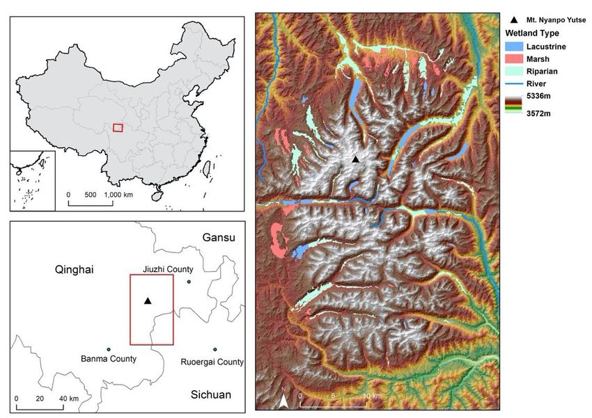
Remote Sens. 2021, 13, 1484                                                                                                            2 of 20

                                      on the Tibetan Plateau, a rate twice the global average [4]. During the same period, about
                                      10% of the alpine wetland on the Tibetan Plateau was lost [5]. If this severe warming trend
                                      continues, a simulation suggests that about 35.7% of the wetland might be lost by 2080s,
                                      even under the most optimistic scenario according to the IPCC 4th Assessment Report [6].
                                           However, the trend is heterogeneous for different wetland types in different regions of
                                      the Tibetan Plateau (Table 1). A review by [2] suggests that between 1970 and 2006, the river
                                      and swamp wetland area decreased overall at a rate of 0.23%/a, yet the area of lakes in
                                      inland river basins increased at a rate of 0.17%/a. This trend has since been confirmed by [7].
                                      While rapid climate change is an oft-cited reason for wetland degradation, there is limited
                                      empirical evidence on the mechanisms linking the two patterns [2,4]. Given the uneven
                                      water distribution across the Tibetan Plateau, local wetland responses to climate change
                                      may vary [8]. It has been proposed that the rising temperature is likely to drive wetland
                                      change by widening the water gap between evapotranspiration and precipitation [9],
                                      varying the regime of glacial water influx [10,11], and melting permafrost [12]; however,
                                      debates around the directions and magnitudes of these effects persist [10,13].

                                 Table 1. A Sample of Studies on Wetland Change on the Tibetan Plateau.

   Article               Focus                 Spatial Extent          Timespan                         Main Conclusions
                                                                                         10% loss of wetland across the Tibetan Plateau.
                                                                                            Greatest degradation occurred in Yangtze
                      Area change
     [5]                                    Entire Tibetan Plateau     1967–2014                         source region.
                     Fragmentation
                                                                                        Wetland fragmentation accelerated in Yellow river
                                                                                              headwaters region and Zoige basin.
                                                                                                  Lake area increased of 35.3%.
     [7]              Area change           Entire Tibetan Plateau     1990–2010         River and swamp decreased by with 833.49 km2
                                                                                                       and 2761.30 km2 .
                     Area change
                                                                                         Temperature rise causes drying of wetland and
     [9]           Structure change             Maqu County            1995–2010
                                                                                                  reduction in biodiversity.
                  Vegetation diversity
                                                                                       Changes in evapotranspiration does not completely
                      Area change
    [14]                                         Zoige basin           1967–2011        explain peatland degradation as precipitation >
                        Driver
                                                                                          evapotranspiration during the study period
                                                                                            Lake increase steadily by a small amount
                                                                                               Marsh wetland significant decreases
                                                Three River
    [15]              Area change                                      1976–2013       Wetland in Yangtze River Basin has been decreasing
                                               Source Region
                                                                                       since 2004, while wetland in Yellow River Basin has
                                                                                                         been increasing.
                                                                                        Total area changed (expansion and contraction) by
    [16]              Area change            Mt. Everest Region        1988–2016                         94.5 km2 (5.6%).
                                                                                         Regressive succession occurred in some regions.
                      Area change                                                       Succession between lake, marsh, semi-marsh, and
    [17]                                         Zoige Basin           1977–2001
                      Succession                                                                      grassland was found.
                      Area change                                                              Area decreased in the study period.
    [18]           Structural change             Zoige Basin           2000–2015               Fragmentation varied in the period.
                  Biodiversity change                                                         Vegetation biomass dropped in 2015.
                                                                      1960s–2006         Patterns of changes in the area of lakes differ by
    [19]             Area, number           Entire Tibetan Plateau
                                                                        (maps)                     regions. No consistent trend.
                   Runoff production                                                     Basins with larger wetlands have lower runoff
                 Growing season length                                                      Increasing trend of non-freeze period and
    [20]          Evapotranspiration             Zoige Basin           1985–2007                         growing season.
                  Vertical temperature                                                 Increasing trend in evapotranspiration and vertical
                        gradient                                                                      temperature gradient.
                                                                                          Wetland decreased by 440 km2 , deep wetland
                      Area change
    [21]                                         Zoige Basin           1994–2009           decreased by 78 km2 and humid meadow
                    Type Conversion
                                                                                                     decreased by 80 km2
                      Area change                                                       Wetland steadily converted to other types, mainly
    [22]                                         Zoige Basin           1975–2005
                    Type Conversion                                                      various kinds of grasslands and sandy lands.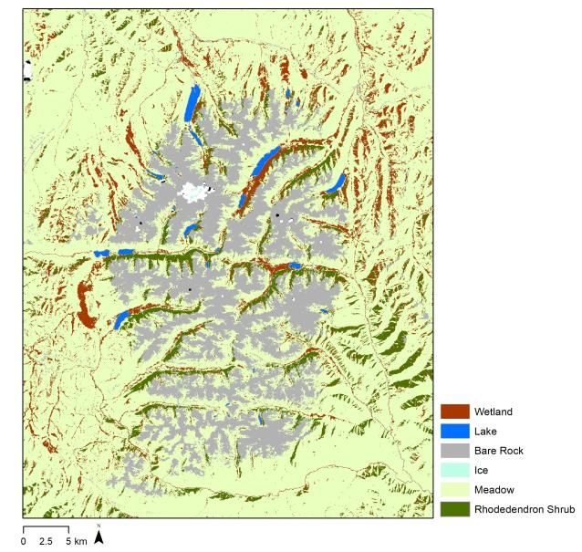
Remote Sens. 2021, 13, 1484                                                                                                           3 of 20

                                                                 Table 1. Cont.

   Article               Focus                  Spatial Extent           Timespan                      Main Conclusions
                                                                                       Degree of wetland degradation is assessed a priori.
                     Soil moisture                                                     Density of pika burrows is a less reliable indicators
    [13]                                        Maduo County                2011
                    Vegetative cover                                                     for wetland change, vegetation cover and soil
                                                                                              moisture content are more reliable.
               Gross-primary production                                                   Simulation shows increasing EVI, LSWI, and
    [23]                                         Zoige Basin             2000–2011
                      Phenology                                                                      growing season GPP
                                                                                          Wetland shrank from 5308 km2 to 4980 km2
                                                                                        Sandy land expanded from 112 km2 to 137 km2
    [24]              Area change                Zoige Basin             1990–2005
                                                                                       Forest land decreased from 5686 km2 to 5443 km2
                                                                                       Grassland degraded from 12,309 km2 to 10,672 km2
                                                                                         The value of ecosystem services dropped from
    [25]           Ecosystem service             Zoige Basin             1975–2015
                                                                                       61.46 × 10⁹ yuan in 1975 to 58.61 × 10⁹ yuan in 2005.

                                             Most recent studies on wetland degradation on the Tibetan Plateau benefit from
                                       remotely sensed datasets, allowing rapid sampling across vast, inaccessible landscapes.
                                       In many cases, remote-sensing data is the only feasible approach for obtaining data over
                                       a wide geographic range. The results of these studies have been used in state-sponsored
                                       conservation campaigns about the Tibetan Plateau, including the establishment last year
                                       of China’s first national park in the Sanjiangyuan region [26–28]. Meanwhile, there is
                                       an emerging trend of community-based conservation campaigns on the Tibetan Plateau
                                       as NGOs and local herders have formed various cooperatives to promote traditional
                                       cultural and ecological practices [29]. The latter movement places more emphasis on local
                                       conservation concerns such as biodiversity monitoring and pasture restoration, and it often
                                       relies on empirical knowledge. While there have been successful attempts to incorporate
                                       remote sensing data in assessing local resource usage and conservation problems [30,31],
                                       it is often difficult to make this information useful for community stakeholders due to
                                       technical constraints, competing interests, and epistemological differences [32].
                                             Furthermore, collecting climate-related ecological changes across spatiotemporal
                                       scales meaningful to community members and local resource managers is challenging
                                       because no one method reliably produces essential data at both fine and broad scales [33].
                                       Most remote-sensing studies (Table 1) focus on large-scale, low-resolution analyses covering
                                       the entire Tibetan Plateau or large topographically flat areas (such as the Zoige basin).
                                       Nevertheless, climate, topographic, and hydrological conditions vary significantly within
                                       the Tibetan Plateau, and there are potentially large variations in wetland changes in
                                       different regions. While studies in large, flat wetlands are valuable, few studies examine
                                       the trends of small, fragmented wetlands in mountainous areas where the habitats’ spatial
                                       heterogeneity can support higher biodiversity. Conservation initiatives and community
                                       planning on the ground require local-scale characterization of wetland changes. The coarse
                                       scale of common remote sensing studies is often insufficient to address these needs.
                                             Another issue in the current wetland remote sensing literature on the Tibetan Plateau
                                       is the varied meanings of the term “degradation.” As [18] points out, wetland degradation
                                       is a complex, integrated process of wetland area, structure, and function change. However,
                                       most of the current studies focus on only one aspect of the multidimensional process, with
                                       many studies concentrating on changes in area [2]. While the areal extent is a fundamental
                                       dimension of wetland changes, our fieldwork on the Tibetan Plateau and interviews with
                                       local herders suggest that the structure and ecological services of some wetlands might
                                       evolve without any apparent change in the area. In addition to changes in the wetland area,
                                       two empirical trends we noticed from our fieldwork are changes in wetland water content
                                       and the succession of vegetation types. A wetland experiencing these internal changes
                                       will serve different ecological functions, host different plant and animal communities, and
                                       affect local herders in different ways than it did originally.
                                             Given the challenges of characterizing wetland changes from remote-sensing data
                                       in the context of climate change, we faced the question of how to provide local conser-
Remote Sens. 2021, 13, 1484 4 of 20
vationists with meaningful climate and wetland trend analyses on an ecological scale
that interested them the most. To address this question, we explored the use of publicly
available satellite image and climate records to remotely assess temporal trends in small,
fragmented wetlands in a rugged mountainous region of the Eastern Tibetan Plateau,
where local herders have reported a widespread decline in wetlands and pasture over the
past 30 years. Specifically, we aimed to collect direct evidence of wetland change from satel-
lite images to determine whether the observed wetland degradation might be driven by
climate change. We did this by examining trends in the wetland area (using Landsat TM),
water content, and vegetation structure (with Sentinel-2 SAR) and by characterizing trends
of regional climate variables using ground weather records of temperature, precipitation,
and potential evapotranspiration (CHIRTSmax for maximum temperature, MODIS for snow
cover fraction and NDVI, ALEXI and SSEBop models for evapotranspiration). While we
acknowledge that there might be better quality remote-sensing data (orthophotos, hyper-
spectral images, and high-resolution images) in commercial or governmental datasets, we
limited our scope to readily available data to reflect the technical and financial constraints
faced by local conservationists. In the context of previous literature, the contribution of
this paper is to examine the value of publicly available satellite datasets in studying the
trend of wetland changes in topographically constrained wetlands.
2. Materials and Methods
2.1. Regional Setting
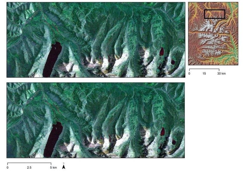
Located on the Eastern Tibetan Plateau, our study site (100◦ 900 –101◦ 400 E, 32◦ 900 –
33◦ 550 N) is a geomorphologically unique region surrounding Mt. Nyanpo Yutse (5368
m) on the border between Qinghai and Sichuan provinces, China (Figure 1). The region
is characterized by an 820 km2 granite dome rising 500–800 m above the surrounding
peneplain, with the highest peaks above 5100 m still covered by 5.2 km2 of modern
glaciers [34]. Multiple Pleistocene glaciations deeply incised into granite batholith, leaving
a distinctive glacial landform of U-shaped valleys, cirque lakes, and granite moraines.
Below the near-vertical granite cliffs, alpine meadow covers much of the aeolian sandy
silt between 3500 and 4300 m, providing pasture for nomadic herders who have been
migrating across the region for at least 2200 years, based on palaeoecological records [35].
The region’s climate is controlled by the East Asian monsoon and can be divided into
cold and warm seasons, with an annual mean temperature of 0.1 ◦ C and an annual mean
precipitation of 760 mm [31]. It is one of the wettest regions in Qinghai Province, but ~80%
of the annual precipitation occurs from May to October, making the cold season very dry
(Figure 2). The steep elevation and climate gradients in the region lead to a diversity of
micro ecosystems, providing habitats for some endangered species such as snow leopard
(Panthera uncia), Tibetan bunting (Emberiza koslowi), black-necked crane (Grus nigricolis),
and an endemic Himalayan poppy (Meconopsis barbiseta) [36].
Hydrographically, Mt. Nyanpo Yutse is part of the NW–SE Bayan Har Mountains
that divide the Yangtze River watershed to the south and the Yellow River watershed to
the north. With elevation gradually decreasing from the center of the study region to the
periphery, rivers radiate outward along the glacial trough valleys. At the flat bottom of
the valleys or where moraines impede water flow, wetlands may develop. Based on their
geological settings, we classified wetlands in our study area into three types: (1) “lacustrine
wetlands”, which surround open cirque lakes that are directly controlled by the water
level in the lakes; (2) “riparian wetlands”, which develop along the riverbed of braided
rivers at the bottom of the glacial trough valleys or on alluvial fans at valley openings;
and (3) “marsh wetlands” with thick peat layers, which are found in glacial basins to the
north and east of the study region (see the right panel of Figure 1 for details). In this
study, we only focused on riparian wetlands and marsh lands since the narrow width of
lacustrine wetlands around the lake often makes them difficult to separate from open water
on medium-resolution satellite images.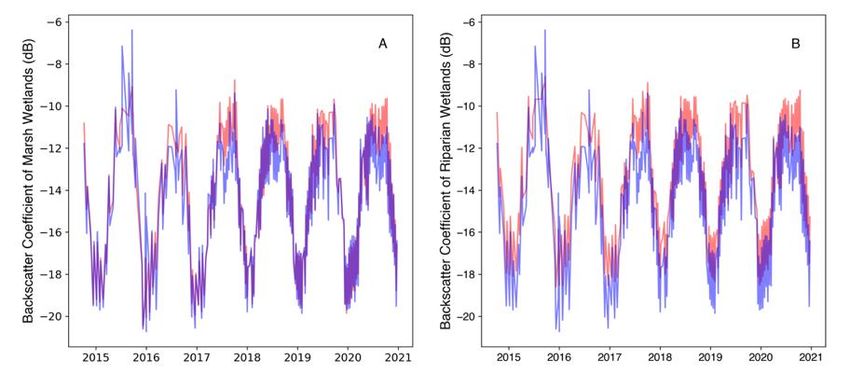
tation of 760 mm [31]. It is one of the wettest regions in Qinghai Province, but ~80% of the
annual precipitation occurs from May to October, making the cold season very dry (Figure
2). The steep elevation and climate gradients in the region lead to a diversity of micro
ecosystems, providing habitats for some endangered species such as snow leopard (Pan-
Remote Sens. 2021, 13, 1484 thera uncia), Tibetan bunting (Emberiza koslowi), black-necked crane (Grus nigricolis),5 and
of 20
an endemic Himalayan poppy (Meconopsis barbiseta) [36].
Remote Sens. 2021, 10, x FOR PEER REVIEW 6 of 22
3) “marsh wetlands” with thick peat layers, which are found in glacial basins to the north
Figure
and east1.ofMaps
Figure of the study
the study
Maps study area.
regionarea. The
(seeThe map
themap onpanel
right
on theright
the right showsthe
ofshows
Figure the locations
1 locations
for ofofthree
details). three types
In this of of
study,
types wet-
we
wetlands
lands based on manual classification from Landsat remote sensing images. Lacustrine
only focused on riparian wetlands and marsh lands since the narrow width of lacustrine to
based on manual classification from Landsat remote sensing images. Lacustrine wetlands
wetlands refer
refer
wetlandsto the
the open openofwater
around
water the
cirqueof lakes
lake cirque
often lakes
and theand
makes the surrounding
them difficult
surrounding to semi-submerged
separate from
semi-submerged ground.
open
ground. Marsh
water
Marsh wet-
on me-
wetlands are
lands are wetlands distributed along the banks of rivers and cover the bottom of the glacial val-
dium-resolution satellite
wetlands distributed along images.
the banks of rivers and cover the bottom of the glacial valleys.
leys.
15
Hydrographically, Mt. Nyanpo Yutse is part of the NW–SE 160
Bayan Har Mountains
that divide the Yangtze River watershed to the south and the Yellow River watershed to
the north. With elevation gradually decreasing from the center of the study region to the
10
periphery, rivers radiate outward along the glacial trough valleys. At the flat bottom of Monthly Mean Precipitation (mm)
Monthly Mean Temperature(°C)
the valleys or where moraines impede water flow, wetlands may120 develop. Based on their
geological
5 settings, we classified wetlands in our study area into three types: 1) “lacustrine
wetlands”, which surround open cirque lakes that are directly controlled by the water
level in the lakes; 2) “riparian wetlands”, which develop along the riverbed of braided
rivers 0at the bottom of the glacial trough valleys or on alluvial fans
80at valley openings; and
1 2 3 4 5 6 7 8 9 10 11 12
-5
40
-10
-15 0
Figure 2. Thirty-Year Average of Monthly Mean Temperature and Precipitation reported by the
Figure 2. Thirty-Year Average of Monthly Mean Temperature and Precipitation reported by the
weather station
weather station at at Jiuzhi
Jiuzhi county
county (elevation
(elevation 3630
3630 m),
m), 2525
kmkm
toto
thethe northeast
northeast ofof
ourour study
study site.
site.
Given that there is no significant surface water flow into the region, the incoming
Given that there is no significant surface water flow into the region, the incoming
water is almost entirely from rain, snowmelt, and glaciers (Figure 3). As modern glaciers
water is almost entirely from rain, snowmelt, and glaciers (Figure 3). As modern glaciers
cover less than 1% of the study region, we assumed their contribution to the regional water
cover less than 1% of the study region, we assumed their contribution to the regional wa-
budget to be negligible. Thus, we considered rain and snowmelt to be the main sources. The
ter budget to be negligible. Thus, we considered rain and snowmelt to be the main sources.
main water sinks in our region are surface flow, underground flow, and evapotranspiration.
The main water sinks in our region are surface flow, underground flow, and evapotran-
However, without detailed ground monitoring data, we cannot reliably estimate the extent
spiration. However, without detailed ground monitoring data, we cannot reliably esti-
to which these variables have changed over the past decades. Thus, we focused only on
mate the extent to which these variables have changed over the past decades. Thus, we
focused only on evapotranspiration, with the assumption that the latter would be more
directly influenced by climatic drivers such as temperature, wind speed, and relative hu-
midity.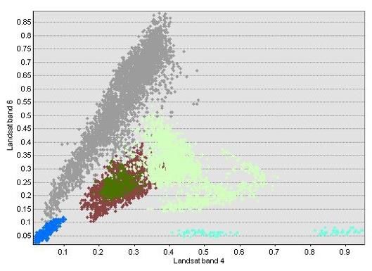
Given that there is no significant surface water flow into the region, the incoming
                              water is almost entirely from rain, snowmelt, and glaciers (Figure 3). As modern glaciers
                              cover less than 1% of the study region, we assumed their contribution to the regional wa-
                              ter budget to be negligible. Thus, we considered rain and snowmelt to be the main sources.
Remote Sens. 2021, 13, 1484
                              The main water sinks in our region are surface flow, underground flow, and evapotran-    6 of 20
                              spiration. However, without detailed ground monitoring data, we cannot reliably esti-
                              mate the extent to which these variables have changed over the past decades. Thus, we
                              focused only on evapotranspiration, with the assumption that the latter would be more
                              evapotranspiration,
                              directly influenced bywith the assumption
                                                      climatic           thatasthe
                                                               drivers such        latter wouldwind
                                                                                 temperature,   be more directly
                                                                                                    speed,       influenced
                                                                                                           and relative   hu-
                              by  climatic drivers such as temperature, wind speed, and relative humidity.
                              midity.

                              Figure 3. A
                              Figure 3.    simplified diagram
                                        A simplified  diagram of
                                                               of water
                                                                   water sources
                                                                         sources and
                                                                                 and water
                                                                                     water sink
                                                                                           sink in
                                                                                                in our
                                                                                                   our study.
                                                                                                       study. The
                                                                                                              The boxes
                                                                                                                  boxes marked
                                                                                                                        marked in
                                                                                                                               in
                              blue are factors estimated in
                                                         in this
                                                            this study.
                                                                 study.

                              2.2. Analysis of Satellite-Based Evidence of Wetland Change
                              2.2. Analysis of Satellite-based Evidence of Wetland Change
                                    Our first goal was to quantify changes in wetland areas by conducting supervised
                                    Our first goal was to quantify changes in wetland areas by conducting supervised
                              classification of Landsat images over our study site (Path: 137, Row: 37). We acquired all
                              classification of Landsat images over our study site (Path: 137, Row: 37). We acquired all
                              Landsat TM, ETM, and OLI images captured between mid-July and mid-August from 1988
                              to 2017 and filtered the images by the percentage of cloud cover. Because of heavy clouds
                              in the summers, we found only five usable images with light cloud cover over the wetlands
                              of interest. These were captured by Landsat 5 TM on 16 August 1996; 14 August 2001; 6
                              August 2004; 27 July 2006; and 25 July 2011. All scenes were preprocessed to the study
                              area’s extent, atmospherically corrected, calibrated to surface reflectance, and normalized
                              to values between 0 and 1. We then applied Landsat QA bands to mask out the clouds
                              and cloud shadows. Based on extensive fieldwork experience in the region and visual
                              interpretation of a Landsat TM image from 2004, we created a training dataset consisting
                              of six land-cover types: wetland, lake, bare rock, ice, meadow, and shrub. The numbers of
                              training pixels for each class were approximately proportional to the area of the class, and a
                              signature file was computed independently for each image over the same training regions.
                              We used this training sample to train a maximum-likelihood classifier on bands 1–7 of each
                              Landsat image, and applied the classifier to each image. The algorithm correctly separated
                              bare rocks, glacier, lake, and meadow from other land-use types. Ancillary data were used
                              to distinguish wetlands from upland shrub regions based on the similarity of their spectral
                              signatures. For this purpose, we used 30 m ASTER GDEM to mask out all wetland pixels
                              with an elevation above 4500 m or a slope greater than 20 degrees because surface water
                              cannot easily be contained on sleep slopes, except under special geological settings [37].
                              We masked out all regions where there was a data gap in any of the images and counted
                              the number of pixels classified as wetlands in each image. We then evaluated the accuracy
                              of the classification by constructing confusion matrices against an independent test dataset
                              and calculated Cohen’s kappa as an indicator of reliability.
                                    Next, we examined potential changes in vegetation and water cycles within the
                              wetlands. Due to extensive cloud cover, we apply synthetic aperture radar data to the
                              problem, as it can provide information on water level and the texture of vegetation canopies
                              regardless of cloudiness [38]. In this study, we utilized the Sentinel-1 GRD collection hosted
                              on Google Earth Engine. This dataset has been preprocessed through a sequence of
                              steps, including updating orbit metadata, border noise removal, thermal noise removal,
                              radiometric calibration, and terrain correction using the protocols in Sentinel-1 Toolbox. The
                              raw unitless backscatter coefficients were converted to normalized backscatter coefficients
                              in dB [39]. We filtered the dataset to extract all images over the study area on the descending
                              orbit acquired through the Interferometric Wide Swath mode. VV data has been available
                              since October 2014. Using both ground-truth data and Landsat images, we manually traced
                              out the contours of visible marsh and riparian wetlands (assuming that the boundaries of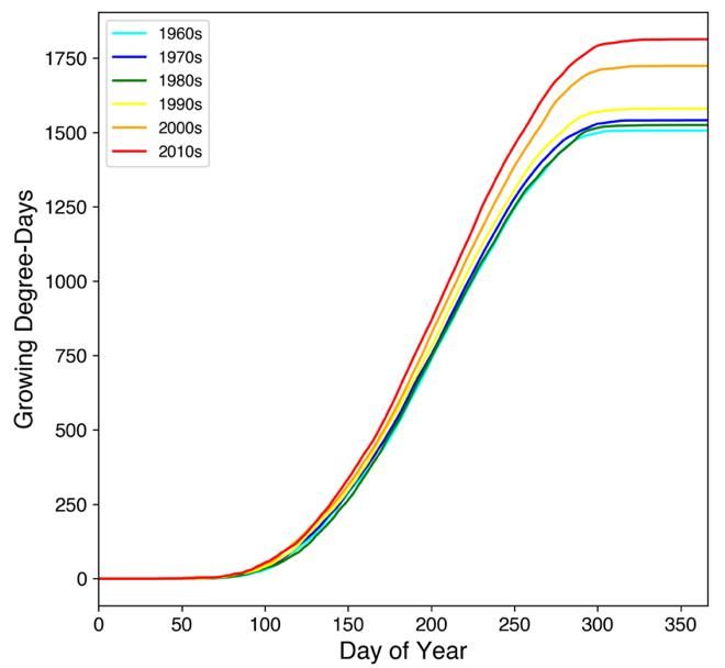
Remote Sens. 2021, 13, 1484                                                                                          7 of 20

                              wetland stayed constant over time, which was supported by the Landsat data). We then
                              calculated the time series of VV backscatter coefficients averaged over each type of wetland.

                              2.3. Analysis of Potential Climate Drivers of Wetland Change
                                    In addition to collecting direct evidence of wetland change, we examined the potential
                              climate factors that may drive wetland degradation. A significant challenge for analyzing
                              climate trends in our study area was the paucity of ground monitoring data. The closest
                              weather station is located at 25 km to the northwest at the Jiuzhi county seat, which has a
                              daily record of temperature, precipitation, wind speed, relative humidity, and sunshine
                              hours from 1959.
                                    To improve the spatial resolution of climate records, we supplemented the ground
                              observations with satellite data and modeling products. For temperature, we explored the
                              CHIRTSmax gridded station-corrected satellite derived monthly-averaged daily maximum
                              temperature [40], but we found the CHIRTSmax data contained anomalies and was incon-
                              sistent with ground observations in our area of interest. Thus, the single-point observation
                              was determined to be our best estimate of regional temperature trends for our local-scale
                              application. We employed monthly snow cover fraction data derived from MODIS ob-
                              servations to inform estimates of spring meltwater. MODIS snow covered area data were
                              validated as having about 90% accuracy over the Tibetan Plateau [41].
                                    As previous studies have shown that the increase in evapotranspiration associated
                              with temperature rise is a likely driver of climate-induced degradation on the Tibetan
                              Plateau, we took extra caution in constructing the evapotranspiration records in our study
                              area. In this study, we examined three kinds of indicators: (1) “actual evapotranspiration”
                              (ETa ), the amount of water evaporated from the vegetation within our study region; (2)
                              “reference crop evapotranspiration” (ETref ), the maximum amount of water capable of being
                              evaporated from the soil and transpired from vegetation [42]; (3) “changes in phenology”
                              because a longer growing season can be a potential driver of greater evapotranspiration.
                                    For actual evapotranspiration, we examined the 10-day average actual evapotranspira-
                              tion product of the Simplified Surface Energy Balance model parameterized (SSEBop), and
                              the 8-day averaged actual evapotranspiration product from Atmosphere-Land Exchange
                              Inverse model (ALEXI). Combining 10-day average MODIS thermal imagery surface tem-
                              perature, PRISM data for air temperature, and reference evapotranspiration from GDAS,
                              the SSEBop model provides a thermally based estimation of ETa based on predefined,
                              seasonal dynamic “hot” and “cold” boundary conditions unique for each pixel [43]. The
                              ALEXI model incorporated a 7-day clear sky MODIS thermal dataset into a two-source
                              land-surface representation model consisting of both soil and canopy to derive the evap-
                              otranspiration estimate [44]. For reference crop evapotranspiration, we used the daily
                              average weather variables recorded by Jiuzhi meteorological station and the Penman-
                              Monteith equation recommended by FAO to compute Erc each day and calculated annual
                              mean values. We did not use the pan-evaporation data at Jiuzhi meteorological station
                              because of the inconsistent use of different evaporation pans at the meteorological station
                              and the lack of accurate calibration data.
                                    Finally, we examined phenology data to determine if the trend of lengthening the
                              growing season might drive up water demand in our region of interest. We calculated
                              the growing degree-days in our region of interest, which is defined as GDD = (Tmax −
                              Tmin )/2 if (Tmax − Tmin )/2 > Tbase or 0 if otherwise [45]. A base temperature Tbase = 0 ◦ C
                              was selected as our study region lies in the cold climate region [46]. We also computed
                              the normalized difference vegetation index (NDVI) over our study region using MODIS
                              16-day, clear sky observation. We studied the trends on specific days during the spring and
                              fall to examine if there were an indication of advancement in spring green-up or delay in
                              fall senescence.
Remote Sens. 2021, 13, 1484 8 of 20
x FOR PEER REVIEW 9 of 22
3. Results
3.1.change
not observe a visible Wetlandin Area
the wetland boundary, suggesting that the actual area of
wetlands may be mostly stable. supervised classification (Figure 4), the wetland area in our study region
Based on a
was 61.4 km2 , 63.9 km2 , 86.4 km2 , 63.9 km2 , and 77.9 km2 in 1996, 2001, 2004, 2006, and
2011, respectively. The classification accuracies before and after filtering were evaluated
Table 2. Confusion Matrix of Supervised Classification for Landsat 5 TM image in 2004.
in Tables 2 and 3, using ground-truth points selected based on first-hand field knowledge
and visual interpretation of a recent Sentinel-2 image. The Cohen’s kappa coefficient was
User’s Ac-
Wetland0.77 forLake
all five landRock
cover types Meadow Shrub
(ice was excluded because Total
of the very small number of
pixels available), and 0.81 for wetland/non-wetland after reclassification curacy
and filtering.
Wetland 78 These results
0 were skewed 0 4
by the varying degree7 of cloud cover
89 in different
0.88scenes. In
Lake 0 particular,34the Landsat 0image from 2004 0 is the only 0cloud-free image,
34 so it has a1much larger
number of effective training samples than the other images, which resulted in a greater
Rock 1 number of 8 pixels being80classified as wetland.
0 0
A comparison 89 wetland
between 0.90
classification
Meadow 12 at the beginning
0 0 end of the69
and the study period30 111 suggests0.62
(1996 and 2011) that there are
Shrub 2 no consistent
0 spatial patterns
0 of pixels
0 indicating
28 wetland gain
30 or wetland loss, so the
0.93
observed variations in the total area of pixels classified as wetland is more likely due to
Total 93 classification
42 errors and 80 cloud cover 73than actual65 353wetland area (Figure 5).
changes in the
Producer’s Comparing Landsat images in different years to our ground-truth data, we did not observe
0.84 a visible0.81
change in the 1 0.95 suggesting
wetland boundary, 0.43 that the actual area of wetlands may
Accuracy
be mostly stable.
Kappa 0.77
(a) (b)
Figure 4. (a) Maximum-likelihood classification results of Landsat 5 TM image over the study area on 6 August 2004.
Figure 4. (a) Maximum-likelihood classification results of Landsat 5 TM image over the study area
(b) The scatterplot of Landsat band 4 (near infrared) and band 6 (thermal infrared).
on August 6, 2004. (b) The scatterplot of Landsat band 4 (near infrared) and band 6 (thermal infra-
red).Remote Sens. 2021, 13, 1484 9 of 20
Table 2. Confusion Matrix of Supervised Classification for Landsat 5 TM image in 2004.
User’s
Wetland Lake Rock Meadow Shrub Total
Accuracy
Wetland 78 0 0 4 7 89 0.88
Lake 0 34 0 0 0 34 1
Rock 1 8 80 0 0 89 0.90
Meadow 12 0 0 69 30 111 0.62
Shrub 2 0 0 0 28 30 0.93
Total 93 42 80 73 65 353
Producer’s Accuracy 0.84 0.81 1 0.95 0.43
Kappa 0.77
Table 3. Confusion Matrix After Filtering by Elevation and Slope for 2004 Image.
Non-Wetland Wetland Total User’s Accuracy
Non-Wetland 253 7 260 0.97
Wetland 18 75 93 0.81
Total 271 82 353
Producer’s Accuracy 0.93 0.91
Remote Sens. 2021, 10, x FOR PEER REVIEW 10 of 22
Kappa 0.81
Figure 5. Composite of wetland classification results on 16 August 1996 and 25 July 2011. Grey pixels
Figure 5. Composite of wetland classification results on August 16, 1996 and July 25, 2011. Grey
represent
pixels areas areas
represent classified as wetland
classified in bothin1996
as wetland bothand 2011,
1996 andblack
2011,pixels
black represent areas not
pixels represent classified
areas not
classified as wetland in either year. Red pixels represent areas classified as wetland in 1996 butCyan
as wetland in either year. Red pixels represent areas classified as wetland in 1996 but not 2011. not
pixels
2011. represent
Cyan pixels areas classified
represent areasas wetlandasinwetland
classified 2011 butinnot
20111996.
butWhite pixels
not 1996. are pixels
White regionsare
removed
re-
due to
gions cloud cover.
removed due to cloud cover.
3.2. Wetland
Table Vegetation
3. Confusion Matrixand Water
After Filtering by Elevation and Slope for 2004 Image.
Figure 6 displays the seasonal pattern of Sentinel-1 SAR backscattering coefficients of
Non-Wetland
wetlands in the northern part Wetland
of our study area. The red band Total User’s Accuracy
displays time-averaged nor-
Non-Wetland
malized 253in spring (15 March–15
backscattering coefficient 7 April),260
the green band0.97
shows that
for late Wetland
spring (10 May–1 June),18 75 shows that for
and the blue band 93 summer (15 July–15
0.81 Au-
Total
gust). Note 271 of the image82
that all vegetated parts 353 color, which suggests
have a bluish-green
increased
Producer’sbackscattering
Accuracy during periods of vegetation
0.93 0.91 growth. In particular, the wetland
Kappa 0.81
3.2. Wetland Vegetation and Water
Figure 6 displays the seasonal pattern of Sentinel-1 SAR backscattering coefficientsRemote Sens. 2021, 13, 1484 10 of 20
has a brighter color than the surrounding area, suggesting that during the growing season
the backscatter is higher in the water-flooded wetland than the adjacent grassland. This is
not surprising given the presence of a microwave double bounce between wetland water
and hydrophytes. Therefore, a higher backscatter coefficient is indicative of the presence of
water and/or hydrophyte in the wetland. This seasonal cycle is clear in the normalized
Remote Sens. 2021, 10, x FOR PEER REVIEW
VV backscattering coefficients averaged across all the marsh and riparian wetlands 11 in
of 22
our
Remote Sens. 2021, 10, x FOR PEER REVIEW
study region (Figure 7). However, the data did not demonstrate a multi-year trendofthat
11 22
would indicate interannual changes in wetland content or vegetation structure.
Figure 6. False color Sentinel-1 VV image showing distinctive seasonal hydrological and vegeta-
Figure
Figure
tion patternsFalse
6.6.False colorSentinel-1
color Sentinel-1
of wetlands comparedVVimage
VV image
with showing
showing
the distinctive
distinctive
surrounding seasonal
seasonal
grassland hydrological
hydrological
in 2019 and
(top) andand vegetation
2010vegeta-
(bot-
tion patterns
patterns
tom). of wetlands
of wetlands compared
compared withwith the surrounding
the surrounding grassland
grassland in 2019
in 2019 (top)(top)
andand
20102010 (bot-
(bottom).
tom).
Red:
Figure7.7.Red:
Figure Timeseries
Time seriesofofbackscatter
backscattercoefficients
coefficientsofofVV
VVbands
bandsaveraged
averagedover
overall
allmarsh
marshwet-
wetlands
Figure
lands (A)
(A) and7. and
Red:riparian
Time
riparian series of(B).
wetlands
wetlands backscatter
(B). Blue:
Blue: coefficients
TimeTime of of
series
series ofVV bandscoefficients
averaged
backscatter
backscatter over
coefficients ofallVV
of VV marsh wet-
bands
bands aver-
averaged
lands
aged (A)
overover and riparian
samples
samples wetlands
of grassland
of grassland in(B).
in the theBlue:
studystudy Time series of backscatter coefficients of VV bands aver-
region.
region.
aged over samples of grassland in the study region.
3.3.Meteorological
3.3. MeteorologicalRecord Record
3.3. Meteorological
The average Record
daily mean temperature ◦ C from 1959
The average daily mean temperature recorded
recorded
◦
atatJiuzhi
Jiuzhiincreased
increased byby 2.362.36 C from
to 2017,
1959 to The with
average
2017,
an averagemean
with daily
rate of increase of recorded
0.04 C per year (F1,56
rate of increase of 0.04atCJiuzhi
an average temperature
= 150.3,by
increased
per year
pRemote Sens. 2021, 13, 1484 11 of 20
(F1,56 = 3.45, p = 0.07). The increase in minimum temperature was significant in both
January (F1,57 = 40.69, p < 0.0001) with rate of 0.077 ◦ C per year and July (F1,57 = 9.64,
p = 0.003) with a rate of 0.028 ◦ C per year. However, CHIRTSmax data did not show a
significant increase in daily maximum temperature averaged across all months from 1983
to 2016 in the northern part of the study region, including the location of the meteoro-
logical station. A positive trend is observed in CHIRTSmax for January daily maximum
temperature (p < 0.05), and the rate of increase gradually declines from 0.046 ◦ C per year
in the southwest to 0.025 ◦ C per year in the northeast of the study region. During the same
period, there was no significant change in annual total precipitation (F1,56 = 1.44, p = 0.24),
but the relative humidity had a significant decline (F1,56 = 14.57, p = 0.0003). The wind
speed showed an increasing trend from around 1.8 to 2.4 m/s from the 1970s to 1980s, and
it fell back to about 1.7 m/s at the beginning of the 2000s before increasing slightly
Remote Sens. 2021, 10, x FOR PEER REVIEW
in the
13 of 22
late 2000s (Figure 8).
Figure
Figure 8. Time Series of Weather Data8atTime Series
Jiuzhi of Weather Data at Jiuzhi Station
Station.
3.4. Snow Cover FractionRemote Sens. 2021, 13, 1484 12 of 20
3.4. Snow Cover Fraction
Trends in MODIS snow cover fraction from 2000 to early 2019 are presented in Figure 9.
The monthly cover snow cover in our region showed variations from year to year, yet there
was no multiannual trend in the data (F1,16 = 0.57, p = 0.46). Figure 9B–D shows the timing
Remote Sens. 2021, 10, x FOR PEER REVIEW 14 of 22
of snow cover reduction in spring, which would affect the rate of meltwater influx, but,
again, there is not a clear multiannual trend.
Figure 9. (A) MODIS snow cover fraction from March 2000 to February 2019. (B–D) Time series for
Figure
March,9.April
(A) MODIS snow
and May cover fraction from March 2000 to February 2019. (B-D) Time series for
respectively.
March, April and May respectively.
3.5. Evapotranspiration Trends
3.5. Evapotranspiration
Regional averageTrends evapotranspiration modeled by ALEXI from 2003 to 2016 is pre-
sented in Figure
Regional 10. While
average the data suggested
evapotranspiration a clearby
modeled seasonal
ALEXI cycle,
from there
2003 towas no pattern
2016 is pre-
in the in
sented annual
Figure total evapotranspiration
10. While (F1,12 a= clear
the data suggested p = 0.94),cycle,
0.01, seasonal which varied
there wasfrom 380 to
no pattern
490
in themm during
annual the evapotranspiration
total study period. The SSEBop model
(F1,12=0.01, (Figurewhich
P=0.94), 11), onvaried
the other hand,
from 380showed
to 490
regional
mm average
during evapotranspiration
the study period. The SSEBop for only
model about half 11),
(Figure of the
onALEXI
the other model’s
hand, estimate,
showed
regional average evapotranspiration for only about half of the ALEXI model’sthere
averaging from 130 to 230 mm per year. Note that from April to May 2005, were
estimate,
records with abnormally high evapotranspiration values. However,
averaging from 130 to 230 mm per year. Note that from April to May 2005, there were a cross-check with the
weather data in this period revealed no anomalous deviation in temperature,
records with abnormally high evapotranspiration values. However, a cross-check with the precipitation,
or winddata
weather speed in compared
this periodwith the multiannual
revealed no anomalous mean. If we replace
deviation the anomalies
in temperature, with
precipita-
five-year medians, then there is a significant positive trend (F
tion, or wind speed compared with the multiannual mean. If we replace the anomalies1,16 = 4.48, p = 0.05). The
reference crop evapotranspiration is about twice the actual evapotranspiration
with five-year medians, then there is a significant positive trend (F1,16=4.48, P=0.05). The estimated by
reference crop evapotranspiration is about twice the actual evapotranspiration estimateda
ALEXI and about four times the actual evapotranspiration estimated by SSEBop. There is
significant
by ALEXI and positive
abouttrend in thethe
four times reference crop evapotranspiration
actual evapotranspiration (F1,56by
estimated = 16.4, p = 0.0002)
SSEBop. There
is a significant positive trend in the reference crop evapotranspiration (F 1,56=16.4, P=0.0002)
between 1959 and 2017 (Figure 12). The reference crop is positively correlated with annual
average daily maximum temperature (F1,56=62.5, PRemote Sens. 2021, 13, 1484 13 of 20
between 1959 and 2017 (Figure 12). The reference crop is evapotranspiration positively
correlated with annual average daily maximum temperature (F1,56 = 62.5, p < 0.0001),
daily maximum temperature (F1,56 = 6.47, p = 0.014), daily mean temperature (F1,56 = 15.7,
10, x FOR PEER REVIEW 15 of 22
p = 0.0002), and sunshine hours (F1,56 = 69.2, p < 0.0001). Furthermore, the reference crop
10, x FOR PEER REVIEW 15 of 22
evapotranspiration is negatively correlated with relative humidity (F1,56 = 37.5, p < 0.0001)
but not with wind speed (F1,56 = 0.00, p = 0.98).
Figure 10. (A) Annual mean daily average actual evapotranspiration modeled by ALEXI data from
Figure 10. (A) Annual
Figure mean daily average actual evapotranspiration modeled by ALEXI data fromby 2003 to 2017data
(B) Daily
2003 to10. (A)(B)
2017 Annual
Daily mean
ALEXIdaily average actual evapotranspiration
evapotranspiration on different date ofmodeled
year from 2003ALEXI from
to 2017, with
ALEXI evapotranspiration on different date of year from 2003 to 2017, with darker lines representing
2003 to 2017 (B) Daily ALEXI evapotranspiration on different date of year from 2003 to 2017, with more recent years.
darker lines representing more recent years.
darker lines representing more recent years.
Figure 11. (A) Annual mean daily evapotranspiration from 2003 to 2020 (B) Daily SSEBop evapotranspiration on different date of
Figure 11. (A) Annual mean daily evapotranspiration from 2003 to 2020 (B) Daily SSEBop evapo-
yearFigure
from 2003 to (A)
11. 2020,Annual
with darker linesdaily
mean representing more recent years. from 2003 to 2020 (B) Daily SSEBop evapo-
evapotranspiration
transpiration on different date of year from 2003 to 2020, with darker lines representing more re-
transpiration
cent years. on different date of year from 2003 to 2020, with darker lines representing more re-
cent years.Remote Sens. 2021, 13, 1484 Figure 11. (A) Annual mean daily evapotranspiration from 2003 to 2020 (B) Daily SSEBop evapo- 14 of 20
transpiration on different date of year from 2003 to 2020, with darker lines representing more re-
cent years.
Remote Sens. 2021, 10, x FOR PEER REVIEW 16 of 22
days remained mostly the same from the 1960s to 1980s, but it dramatically increased in
the 1990s. The greatest shift in growing-degree days happened between the 1990s and
2000s, where there was a sharp increase from 1580 to 1723 degree-days (Figure 13).
The MODIS 16-day averaged NDVI recorded between 2000 and 2018 suggested an
advancement
Figure12.
Figure 12.(A) in spring
(A)Time
Timeseries phenology
seriesofof referencecrop
reference thatevapotranspiration;
crop was reflected by (B)
evapotranspiration; an upward
(B) Relation trend inreference
Relation between
between interannual
reference crop
NDVI
crop on specific dates
evapotranspiration
evapotranspiration and andduring
annual
annual the
mean meanspring. A rising trend was observed in NDVI recorded
temperature.
temperature.
on March 22 (F1,17=9.43, P=0.007) and April 7 (F1,17=8.57, P=0.0094) but not on March 6
3.6.
3.6.
(F Phenology
Phenology
1,17 =0.73, P=0.40) or April 23 (F=0.03, P=0.87). Thus, the rising trend was only observed
during Between 1960and
an approximate
Between 1960 and2017,
2017,the
32-day the totalgrowing
period
total growing
during degree-days
the early phase
degree-days inin
ofour region
theregion
our ofofinterest
greening-up interest in-
but in-
not
creased
during from
the 1506
entire in the
spring 1960s
(Figure to 1813
14). A in the
delay 2010s.
in fall The decade-averaged
phenology, however,
creased from 1506 in the 1960s to 1813 in the 2010s. The decade-averaged growing-degree growing-degree
was not observed
days
in theremained mostly
data (Figure 15)the
as same
no NDVIfromtrend
the 1960s
was to 1980s, but
observed onitAugust
dramatically increased
13 (F1,17 in the
=0.01, P=0.93),
1990s. The greatest shift in growing-degree days happened between the 1990s
August 29 (F1,17=0.19, P=0.67), September 14 (F1,17=0.14, P=0.71), or September 30 (F1,17=0.13, and 2000s,
where
P=0.72).there was a sharp increase from 1580 to 1723 degree-days (Figure 13).
Figure 13. Cumulative growing degree-days by decades.
The MODIS 16-day averaged NDVI recorded between 2000 and 2018 suggested an
advancement in spring phenology that was reflected by an upward trend in interannual
NDVI on specific dates during the spring. A rising trend was observed in NDVI recorded
on 22 March (F1,17 = 9.43, p = 0.007) and 7 April (F1,17 = 8.57, p = 0.0094) but not on 6
March (F1,17 = 0.73, p = 0.40) or 23 April (F = 0.03, p = 0.87). Thus, the rising trend was only
observed during an approximate 32-day period during the early phase of the greening-up
but not during the entire spring (Figure 14). A delay in fall phenology, however, was not
observed in the data (Figure 15) as no NDVI trend was observed on 13 August (F1,17 = 0.01,
p = 0.93), 29 August (F1,17 = 0.19, p = 0.67), 14 September (F1,17 = 0.14, p = 0.71), or 30
September (F1,17 = 0.13, p = 0.72).Remote Sens. 2021, 13, 1484 15 of 20
Remote Sens. 2021, 10, x FOR PEER REVIEW 17 of 22
Remote Sens. 2021, 10, x FOR PEER REVIEW 17 of 22
Figure 14.
Figure 14.Regional-averaged
Regional-averaged16-day MODIS
16-day NDVI
MODIS on selected
NDVI datesdates
on selected in thein
spring.
the spring.
Figure 14. Regional-averaged 16-day MODIS NDVI on selected dates in the spring.
Figure 15. Regional-averaged 16-day MODIS NDVI on selected dates in the fall.
Figure
Figure15.
15.Regional-averaged
Regional-averaged16-day MODIS
16-day NDVI
MODIS on selected
NDVI dates dates
on selected in the in
fall.the fall.Remote Sens. 2021, 13, 1484 16 of 20
4. Discussion
This study was motivated by local herder reports of wetland degradation in our study
area. Based on these reports, we expected to find evidence in optical or radar satellite
images of changes in wetland area or water content or shifting vegetation structure in the
wetland that would match the ground reports. Given previous studies on climate trends
on the Tibetan Plateau, we also expected to identify potential climate drivers to explain
the reported changes. However, the Landsat records showed no substantive change in our
study area. The C-band SAR images of Sentinel-1 were only available for recent years, but
they also indicated no significant interannual difference in the backscatter coefficients of
the wetland. Thus, remote sensing presented a different picture of the wetlands than the
testimonies from local herders.
On the other hand, the climate record showed a mixed result that partially supported
the existence of climate factors that may drive up water demand in the wetlands. Although
we observed no net change in precipitation in approximately the last 60 years or the snow
cover fraction over the last 20 years, we did see some evidence of rising evapotranspira-
tion and an extension of the growing season. In particular, one of the two satellite-based
diagnostic evapotranspiration models showed an upward trend in actual evapotranspi-
ration, and the calculated annual reference crop evapotranspiration shows a total of 55
mm increase from 1959 to 2017. At the same time, both MODIS NDVI and the growing
degree-days data point to a lengthening of the growing season, which might be another
factor that drives up the water demand in the wetland.
Analysis of Climate Trends
From a climate perspective, the study region’s trends exemplified the widespread
warming patterns on the Tibetan Plateau. The magnitude of temperature rise at Jiuzhi was
much more significant in the winter than in the summer, which is in agreement with earlier
studies that found the winter warming (0.32 ◦ C per decade) to be twice that of the annual
mean temperature (0.16 ◦ C per decade) [3]. We also found a larger and more consistent
increase in the daily minimum temperature than in the daily maximum, suggesting that
warming had a more substantial effect on reducing the net radiative cooling at night.
The trends in reference crop evapotranspiration (Erc ) suggest that the evapotranspira-
tion in our region is temperature-limited rather than precipitation-limited, since (1) there
is a strong correlation between Erc and temperature, but no correlation between Erc and
precipitation; and (2) there is a net water surplus in the region because the estimated
evapotranspiration, regardless of which estimate approach is used, is lower than the total
precipitation. Thus, an increasing temperature would be expected to lead to an increase
in evapotranspiration. Positive trends in ET were observed in wetlands in the wet ar-
eas of the Tibetan Plateau, such as the Zoige basin. In contrast, a negative trend in ET
was observed in wetlands in the hinterland of the Tibetan Plateau, such as the Maidika
wetland and Qiangtang plateau where evapotranspiration is constrained by soil mois-
ture [14,47]. This increasing trend, however, is not consistent with an overall trend of
reference evapotranspiration across the Tibetan Plateau or Eastern China, in general, where
decreasing evapotranspiration is considered to be related to decreasing wind speed caused
by a decline in the intensity of regional monsoon circulation and a decrease in the solar
radiation [42,48,49]. In our study, evapotranspiration was found to be correlated with
sunshine hours but did not correlate with wind speed despite its significant rise and
decline over a period of three decades from 1970 to 2000. A combination of increasing
temperature and decreasing relative humidity is the probable cause of a long-term increase
in evapotranspiration.
It must be noted that the estimates for actual evapotranspiration from energy balance
models should be evaluated with caution. The ALEXI dataset did not take account the
effect of topography and elevation in its model [50]. The SSEBop model, while it did
involve correction for elevation, still performed less optimally in regions with complex
terrain. As its developer suggests, the high variations in ET fraction over mountainous
regions revealed the inherent difficulty of capturing radiation and heat transfer process onRemote Sens. 2021, 13, 1484 17 of 20
steep slopes. This limitation continues to be an area where more research is needed [51].
However, a comparison between our study region with a recent study in Zoige wetland
(100–150 km to the east with an elevation around 700–900 m lower than our region) offers
some very general evidence that the estimates of the model fall within a reasonable range.
The authors of that study estimated the evaporation fraction (Kc)—the ratio between
actual evapotranspiration and reference evapotranspiration—to be 0.40, 0.73, and 0.60 in
grassland and 0.70, 1.09, 0.62 for peatland at Maqu county during the initial, mid-, and end-
section of the growing season [14]. Given that the Maqu weather station is only 83 km to
the northeast and 150 m lower in elevation than Jiuzhi weather station, we may assume that
these values applied to the evaporation fraction for wetland and grassland near the Jiuzhi
township. However, it would be challenging to determine actual evapotranspiration using
the single evaporation fraction approach because the weather records at Jiuzhi township
may not be representative for wetlands located in higher elevation regions.
Our study also provided some insight into the debate on how climate change affects
spring phenology on the Tibetan Plateau. One hypothesis that gained traction in the early
2010s is that strong warming in the winter will slow the fulfillment of chilling requirements
for plants to germinate, thereby causing delays in spring phenology [52]. At the same time,
there was a competing hypothesis suggesting that a continuous advancement in spring
phenology with more substantial advancement at higher altitude [23,46,53]. Our study
seemed to support the second hypothesis although we did not observe a corresponding
delay in the fall phenology. While some researchers have pointed out the observed increase
in spring NDVI might be a false signal caused by decreasing snow cover [54], this did not
appear to be the case since we did not observe a trend in the snow cover fraction during
the same period.
Uncertainties in the Temporal and Spatial Scale
It should be noted that the purpose of this study was not to validate or disprove local
herder’s observations but to provide information that may support local conservation
actions. In particular, the mismatch between the satellite records and the accounts from
the local herders illustrated the importance of being aware of spatial and temporal scales
when combining evidence from different sources to evaluate local environmental change.
In the local herders’ oral accounts, wetland degradation was described in phenomena like
whether yaks can walk across a patch of marshland without sinking into the peat. However,
converting these claims into hypotheses verifiable by satellite images was challenging
because (1) the described phenomenon may happen on a very fine-grained scale below the
resolution of satellite images like Landsat; (2) the specific year and season of the observation
was unknown, while the record of optical remote sensing record contains many gaps due
to severe cloud coverage; (3) the effective resolution of vegetation change or water content
often requires hyperspectral images or active remote sensing, yet many of these products
do not have a record long enough to trace the wetland changes on a decadal scale.
The recent developments of high-resolution optical sensors and the increasing avail-
ability of SAR imagery has led to advances in characterizing water levels in seasonally
inundated vegetation [38]. Our study demonstrated that the time-series of Sentinel-1 image
is capable of capturing seasonal trends in wetlands and differentiating the vegetation
within the wetland from that of the surrounding pastures. While the length of the Sentinel
record is not presently sufficient to reveal long-term changes in wetlands in our study, it
is expected that we may have the potential to characterize details of changes happening
within the wetlands as the record grows in length. However, remote-sensing technology
cannot replace the need for in situ measurements of hydrological and climate variables,
and accurate ground-truth data is needed to improve the reliability of climate models in to-
pographically complex areas. While recognizing the promise of remote-sensing technology
for large-scale wetland mapping, researchers should be aware of the need to verify satellite-
derived data with ground observations and of relevant opportunities and limitations when
applying space-borne observations to the ground.You can also read