Calibration of a combined isotropic-kinematic hardening material model for the simulation of thin electrical steel sheets subjected to cyclic loading
←
→
Page content transcription
If your browser does not render page correctly, please read the page content below
422   Materialwiss. Werkstofftech. 2022, 53, 422–439                                                                        doi.org/10.1002/mawe.202100341

      Calibration of a combined isotropic-kinematic
      hardening material model for the simulation of thin
      electrical steel sheets subjected to cyclic loading
      Kalibrierung eines Materialmodells für die Simulation von
      zyklisch beanspruchten dünnen Elektroblechen unter
      Berücksichtigung kombinierter isotroper-kinematischer
      Verfestigung

      P. Kubaschinski1, A. Gottwalt1, U. Tetzlaff1, H. Altenbach2, M. Waltz1
      The combined isotropic-kinematic hardening model enables the description of the
      cyclic transient elastic-plastic material behaviour of steel. However, the determi-
      nation of the material model parameters and understanding of their influence on
      the material response can be a challenging task. This study deals with the in-
      dividual steps of the material model calibration for the simulation of thin electrical
      steel sheets under cyclic loading. Specific recommendations are made for the de-
      termination of kinematic and isotropic hardening material parameters. In particular,
      the isotropic hardening evolution is described by Voce’s exponential law and a
      simple multilinear approach. Based on the multilinear approach, which allows for
      different slopes in the evolution of the yield surface size, an alternative calibration
      of the isotropic hardening component is proposed. As a result, the presence of the
      yield plateau in the first half cycle can be accurately captured, while convergence
      issues in the material model definition for numerical simulations can be avoided.
      The comparison of simulated load cycles with experimental cyclic tests shows a
      good agreement, which indicates the suitability of the proposed material model
      calibration for electrical steel.

      Keywords: Cyclic plasticity / material model / combined hardening / finite-element
      simulation / electrical steel

      Die Berücksichtigung kombinierter isotroper-kinematischer Verfestigung ermög-
      licht die Beschreibung und Modellierung des transienten elastisch-plastischen
      Werkstoffverhaltens von Stahl. Die Ermittlung der zugrunde liegenden Materialpa-
      rameter und das Verständnis für deren Einfluss auf die Materialantwort stellt je-
      doch häufig eine anspruchsvolle Aufgabe dar. In der vorliegenden Arbeit wird auf
      die einzelnen Schritte bei der Kalibrierung des Materialmodells im Rahmen einer
      Simulation von zyklisch beanspruchten dünnen Elektroblechen eingegangen. Da-
      bei werden konkrete Empfehlungen für die Ermittlung der kinematischen und iso-
      tropen Verfestigungsparameter gegeben. Die Evolutionsgleichung der isotropen
      Verfestigung wird sowohl durch einen Exponentialansatz nach Voce als auch

      1   Technische Hochschule Ingolstadt, Kompetenzfeld                             Corresponding author: P. Kubaschinski, Technische
          Werkstoff- und Oberflächentechnik, Ingolstadt, Ger-                         Hochschule Ingolstadt, Kompetenzfeld Werkstoff- und
          many                                                                        Oberflächentechnik, Esplanade 10, 85049, Ingolstadt,
      2   Otto-von-Guericke-Universität Magdeburg, Institut                           Germany,
          für Mechanik, Magdeburg, Germany                                            E-Mail: Paul.Kubaschinski@thi.de

      This is an open access article under the terms of the Creative Commons Attribution Non-Commercial NoDerivs License, which permits use and distribution in any
      medium, provided the original work is properly cited, the use is non-commercial and no modifications or adaptations are made.
      © 2022 The Authors. Materialwissenschaft und Werkstofftechnik published by Wiley-VCH GmbH                                       www.wiley-vch.de/home/muw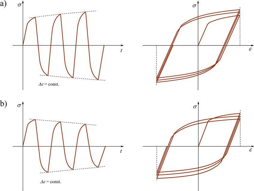
Materialwiss. Werkstofftech. 2022, 53, 422–439                                                      Simulation of thin electrical steel sheets   423

durch einen einfachen multilinearen Ansatz beschrieben. Basierend auf dem multi-
linearen Ansatz, der unterschiedliche Steigungen in der Evolution der Fließfläche
ermöglicht, wird eine alternative Kalibrierung der isotropen Komponente vorge-
schlagen. Dadurch kann das auftretende Fließplateau im ersten Halbzyklus präzi-
se erfasst werden, während Konvergenzprobleme des Materialmodells vermieden
werden. Der Vergleich von simulierten Belastungszyklen mit experimentellen Da-
ten zeigt eine gute Übereinstimmung, was für die Eignung des vorgeschlagenen
Kalibrierungsprozesses für Elektroblech spricht.

Schlüsselwörter: Zyklische Plastizität / Materialmodell / kombinierte Verfestigung /
Finite-Elemente-Simulation / Elektroblech

1 Introduction                                                               city followed by a specific explanation of the mate-
                                                                             rial model calibration for electrical steel.
The rotor of an electric drive, which consists of                            Symmetric strain-controlled cyclic tests are per-
several electrical steel sheets, is exposed to high ro-                      formed to provide stress-strain hysteresis curves for
tational speeds (~ 20.000 min 1) and cyclic loading                          the material parameter determination. To avoid
due to acceleration and deceleration. With typical                           buckling of the thin electrical steel sheets under
sheet thicknesses of only 0.3 mm, the electrical                             compressive forces, the application of an anti-buck-
steel sheets locally exhibit high mechanical stresses                        ling device is necessary which is described more
and strains. In the context of an analytical fatigue                         detailed in this paper. After that, the individual
life assessment, the cyclic elastic-plastic material                         steps of the material parameter determination for
behaviour is evaluated. For this purpose, a suitable,                        the kinematic and isotropic hardening evolution
calibrated material model is required.                                       equations are presented.
    In recent years, different constitutive models and                           Numerical simulations are performed in Abaqus
theories describing the phenomenological mecha-                              comparing the predicted elastic-plastic material be-
nisms of cyclic plasticity have been developed and                           haviour with experimental cyclic tests. The com-
further improved. An overview of several single                              bined isotropic-kinematic hardening model is vali-
yield surface models including the respective evo-                           dated considering cyclic loading both under strain-
lution equations can be viewed in the literature [1].                        and stress-control. As a result, the suitability of the
The choice of the material model for industrial ap-                          determined material parameters can be evaluated.
plications, however, can be a challenging task con-
sidering model complexity, computation time and
experimental data available for the calibration [2].                         2 Constitutive modelling of cyclic
    In this study, the combined isotropic-kinematic                          plasticity: theoretical background
hardening model according to Lemaitre and Cha-
boche is used to describe the transient cyclic elas-                         2.1 Cyclic material behaviour of steel
tic-plastic behaviour of electrical steel [3]. It is
well-established and implemented in most commer-                             The cyclic material behaviour of steel can be char-
cial finite-element applications. The combination of                         acterised by certain phenomenological mechanisms,
isotropic and kinematic hardening allows for an ac-                          which have to be accounted for in the constitutive
curate representation of complex cyclic phenom-                              modelling of cyclic plasticity. Typically, this in-
ena, e. g., cyclic softening/hardening and cyclic                            cludes the Bauschinger effect. Under uniaxial cy-
creep. To ensure a satisfactory alignment between                            clic loading, the yield strength sj0 of a specimen
simulation and actual material behaviour, the mate-                          decreases, after the loading direction is reversed,
rial parameters have to be carefully determined                              Figure 1. Considering the first cycle of a symmetric
based on experimental data.                                                  strain-controlled fatigue test, it can be observed that
    The present work is supposed to give an over-                            the elastic limit while unloading corresponds to the
view of the constitutive modelling of cyclic plasti-                         double of the initial yield strength 2sj0 .

© 2022 The Authors. Materialwissenschaft und Werkstofftechnik published by Wiley-VCH GmbH                         www.wiley-vch.de/home/muw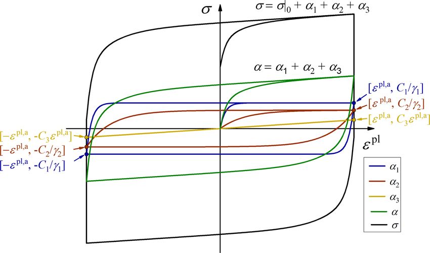
424   P. Kubaschinski                                                                              Materialwiss. Werkstofftech. 2022, 53, 422–439

                                                                                      The stress or strain response of a material under
                                                                                   cyclic loading can change due to microstructural ef-
                                                                                   fects, which results in a decreasing or increasing
                                                                                   deformation resistance [1]. This cyclic softening or
                                                                                   hardening behaviour is material-specific and de-
                                                                                   pends on the loading amplitude as well as the strain
                                                                                   history. The transient material response caused by
                                                                                   cyclic softening/hardening under symmetric strain-
                                                                                   control is associated with changing stress ampli-
                                                                                   tudes, Figure 2. It is usually assumed that the in-
                                                                                   tensity of the response decreases and a stabilised
                                                                                   state is reached.
                                                                                      For unsymmetric load cycles under stress-con-
                                                                                   trol, ratchetting (cyclic creep) has to be considered,
                                                                                   Figure 3a. In the case of uniaxial loading, it can be
                                                                                   measured as accumulation of axial plastic strain
      Figure 1. Influence of the Bauschinger effect on the yield
      strength.                                                                    [1]. The ratchetting rate depends on the cyclic soft-
      Bild 1. Einfluss des Bauschingereffektes auf die Streck-                     ening/hardening and the magnitude of mean stress.
      grenze.                                                                      In contrast, unsymmetric cycles under strain-con-
                                                                                   trol result in mean stress relaxation, Figure 3b.

      Figure 2. Stress-strain response under symmetric strain-controlled cyclic loading, a) cyclic hardening, b) cyclic softening.
      Bild 2. Spannungs-Dehnungsantworten bei symmetrischer dehnungskontrollierter zyklischer Belastung, a) zyklische Verfes-
      tigung, b) zyklische Entfestigung.

      © 2022 The Authors. Materialwissenschaft und Werkstofftechnik published by Wiley-VCH GmbH                         www.wiley-vch.de/home/muw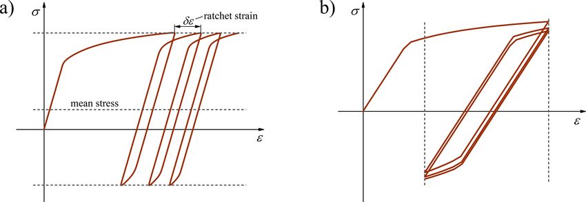
Materialwiss. Werkstofftech. 2022, 53, 422–439                                                                                                                               Simulation of thin electrical steel sheets                                  425

Figure 3. Stress-strain behaviour under unsymmetric cyclic loading, a) ratchetting, b) mean stress relaxation.
Bild 3. Spannungs-Dehnungsverhalten bei unsymmetrischer zyklischer Beanspruchung, a) zyklisches Kriechen, b) Mittel-
spannungsrelaxation.

With increasing number of cycles, the mean stress                            2.2 Nonlinear hardening models
tends to approach zero.
    Besides the mentioned phenomena, the presence                            In Abaqus, the cyclic elastic-plastic material behav-
of the yield plateau (Lüders bands propagation) in                           iour can be described using a combined isotropic-
the first half cycle has to be given particular con-                         kinematic hardening model proposed by Lemaitre
sideration. It can be idealised as a non-hardening                           and Chaboche [3]. A detailed overview of the un-
region between the yield strain ey and the onset of                          derlying constitutive equations of plasticity theory
strain hardening esh , Figure 4 [4]. As long as the                          can be found in the literature [1–6]. For the sake of
onset of the strain hardening is not reached, the                            consistency, the notation used in this paper corre-
yield stress remains more or less constant. After                            sponds to the Abaqus documentation [7]. Hereafter,
load reversal, the yield plateau disappears.                                 the von Mises yield criterion is assumed, which can
                                                                             be expressed as a function of the deviatoric stress
                                                                             tensor S, the deviatoric part of the back stress ten-
                                                                             sor adev and the current yield stress s 0 :
                                                                                  rffiffiffiffiffiffiffiffiffiffiffiffiffiffiffiffiffiffiffiffiffiffiffiffiffiffiffiffiffiffiffiffiffiffiffiffiffiffiffiffiffiffiffiffiffiffiffi
                                                                                   3
                                                                              F ¼            ðS adev Þ : ðS adev Þ                                                                                                                   s0 ¼ 0       (1)
                                                                                   2

                                                                                Moreover, the evolution of the plastic deforma-
                                                                             tion under yielding is described using the asso-
                                                                             ciated flow rule. Depending on the equivalent (ac-
                                                                             cumulated) plastic strain rate �e_ pl , the rate of plastic
                                                                             flow e_ pl can be defined as [7]:
                                                                                                                                                                              rffiffiffiffiffiffiffiffiffiffiffiffiffiffiffiffiffi
                                                                                                    @F pl       pl                                                             2 pl pl
                                                                              e_   pl
                                                                                              ¼ �e_    ; �e_ ¼                                                                           e_ : e_                                                  (2)
                                                                                                    @s                                                                         3

                                                                                The Armstrong-Frederick kinematic hardening
                                                                             model is an extension of Prager’s linear hardening
Figure 4. Presence of the yield plateau in the first half cycle
idealised as non-hardening region, representation according                  rule, which includes an additional recall term to in-
to [4].                                                                      troduce nonlinearity [8, 9]. It is given using the ex-
Bild 4. Vorhandensein des Fließplateaus im ersten Halbzy-                    pression below [3]:
klus idealisiert als nichtverfestigte Region, Darstellung nach
[4].

© 2022 The Authors. Materialwissenschaft und Werkstofftechnik published by Wiley-VCH GmbH                                                                                                                                    www.wiley-vch.de/home/muw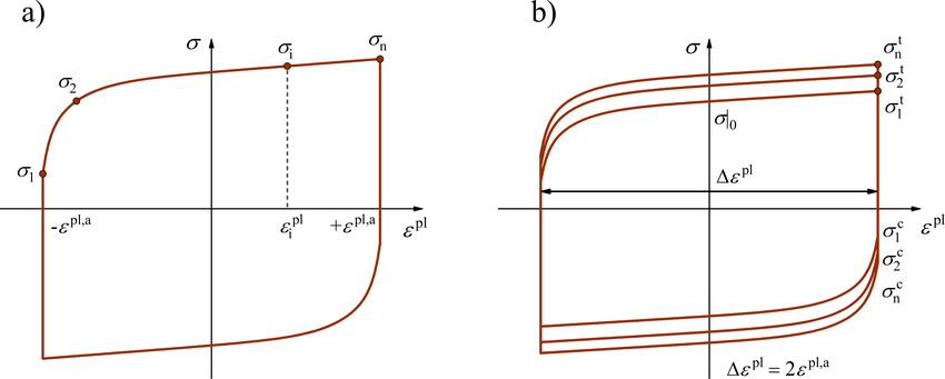
426   P. Kubaschinski                                                                                   Materialwiss. Werkstofftech. 2022, 53, 422–439

              2 pl              pl
                                                                                   strain range increases [3, 6]. Due to that, a super-
      a_ ¼      Ce_        ga�e_                                          (3)      position of several models according to equa-
              3
                                                                                   tion (3) was suggested [6, 10–12]:

         The coefficients C and g represent material pa-                                    X
                                                                                            M
                                                                                                                2
      rameters, where C is the initial kinematic hardening                          a ¼           ai ; a_ i ¼     C e_ pl   gi ai�e_ pl              (6)
                                                                                                                3 i
      modulus and g is defined as the rate at which the                                     i¼1

      kinematic hardening modulus decreases with in-
      creasing plastic deformation [2, 7]. Under propor-                               This results in an improved and more flexible
      tional loading, integrating equation (3) leads to the                        description of the evolution of the back stress a. In
      evolution of the back stress a [3]:                                          analogy to the Armstrong-Frederick evolution mod-
                    �           �                                                  el, equation (5) can be expressed as sum of M back
               C              C        pl pl;0                                     stress components resulting in the Chaboche kine-
       a ¼ y þ a0 y              e ygðe e Þ             (4)
               g              g                                                    matic hardening model [1, 2]:

      where a0 and epl;0 are the initial values for the back                        s ¼ ys 0 þ a ¼ ys 0
      stress and plastic strain at the beginning of the plas-                         XM        �          �
      tic flow. Depending on the direction of plastic flow,                                Ci     ðiÞ   Ci                    ygi ðepl epl;0 Þ       (7)
                                                                                    þ     y þ a0      y      e
      y = 1 for tension and y = -1 for compression. The                               i¼1
                                                                                           gi           gi
      stress is given by the yield condition [3]:
                                                                                       Based on equation (7), the relation between
                   0
      s ¼ ys þ a                                                          (5)      stress and plastic strain can now be determined for
                                                                                   a stabilised cycle. If tension (y = 1) is assumed and
         The Armstrong-Frederick kinematic hardening                               the initial values for the back stress a0 and plastic
      model leads to an unsatisfactory description of the                          strain epl;0 are applied, we receive the upper branch
      cyclic material behaviour when the considered                                of the stress-strain hysteresis curve, Figure 5 [1]:

      Figure 5. Chaboche kinematic hardening evolution with three back stress components, representation according to [1].
      Bild 5. Kinematische Verfestigungsentwicklung nach Chaboche mit drei Rückspannungskomponenten, Darstellung nach
      [1].

      © 2022 The Authors. Materialwissenschaft und Werkstofftechnik published by Wiley-VCH GmbH                                 www.wiley-vch.de/home/muw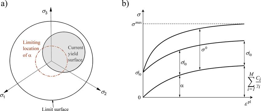
Materialwiss. Werkstofftech. 2022, 53, 422–439                                                                   Simulation of thin electrical steel sheets   427

                                                                                          Alternatively, the evolution of s0 can be ex-
                X
                M
                  Ci �                                             �
s ¼ s þ   0
                           1       2e ð        gi epl þepl;a   Þ                 (8)   pressed by a multilinear relation, where s 0i is the
                i¼1
                      gi                                                               equivalent stress which defines the size of the yield
                                                                                       surface depending on �epl [4, 7]:
                                                                                                             �            �
    The resulting set of parameters (Ci , gi ) should                                  s0 ¼ sj0 þ s0i �epl          sj0                              (11)
not be directly interpreted as material properties,
but as a decomposition of the simpler Armstrong-                                          If isotropic and kinematic hardening evolution
Frederick evolution law [6]. The accurate descrip-                                     equations are both considered simultaneously, we
tion of the cyclic material behaviour using the Cha-                                   receive the combined isotropic-kinematic hardening
boche kinematic hardening model usually requires                                       model, Figure 6. Isotropic hardening covers the
not more than three back stress components ai , Fig-                                   uniform expansion of the yield surface in stress
ure 5. Considering the ratchetting and mean stress                                     space under the development of plastic strain which
relaxation effect, the evolution of the last back                                      can be interpreted as the change of the elastic do-
stress component should be defined according to                                        main [1, 3]. As a result, cyclic softening/hardening
Prager’s linear hardening rule (gM = 0) [1, 3].                                        is accounted for. Kinematic hardening results in a
Hence, equation (8) can be rewritten as:                                               translation of the yield surface in the direction of
                                                                                       the plastic flow which captures the cyclic material
                X
                M 1
                    Ci �                                         �                     behaviour in terms of Bauschinger effect, ratchet-
                                               gi ðepl epl;a Þ
s ¼ s0 þ                   1       2e                                þ CM epl    (9)   ting and mean stress relaxation.
                i¼1
                      gi

    Isotropic hardening can be described using Vo-                                     3 Experimental cyclic testing
ce’s exponential law [13]. The evolution of the
yield surface size s0 is defined as a function of the                                  3.1 Material
equivalent plastic strain �epl considering the initial
yield surface size sj0 , the maximum change in the                                     The material analysed in this study is a fully-proc-
size of the yield surface Q∞ and the speed of stabi-                                   essed non-oriented electrical steel sheet with a
lisation b [3, 6, 7]:                                                                  nominal thickness of 270 μm and the following
                                                                                       composition (mass fraction): 3.32 % silicon, 1.10 %
                                   b�epl
s0 ¼ sj0 þ Q∞ ð1               e           Þ                                    (10)   aluminium, 0.16 % manganese, 0.01 % carbon,

Figure 6. Representation of the combined isotropic-kinematic hardening model, a) in stress-space, b) one-dimensional [7].
Bild 6. Darstellung des kombinierten isotrop-kinematischen Verfestigungsmodells, a) im Spannungsraum, b) eindimensional
[7].

© 2022 The Authors. Materialwissenschaft und Werkstofftechnik published by Wiley-VCH GmbH                                      www.wiley-vch.de/home/muw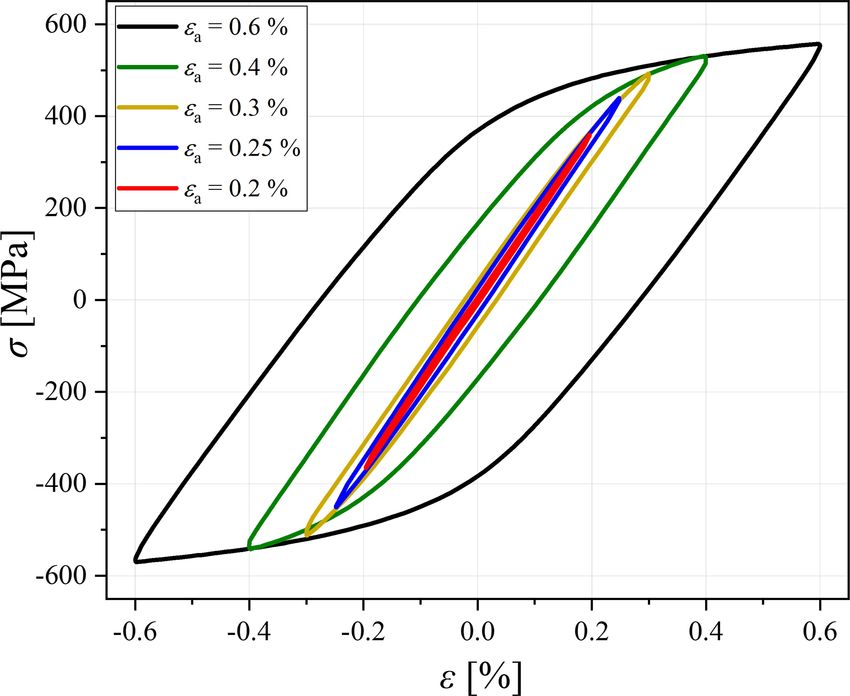
428 P. Kubaschinski Materialwiss. Werkstofftech. 2022, 53, 422–439
0.002 % sulfur, 0.010 % phosphorus, balance iron. teau with an average yield strength of 447 MPa.
Therefore, the material exhibits a ferritic micro- Under quasi-static loading, the material shows a
structure with small non-metallic inclusions. The limited amount of hardening, resulting in a com-
average grain size is approximately 100 μm, de- paratively flat stress-strain curve with an ultimate
termined by electron backscatter diffraction tensile strength of 540 MPa and an elongation at
(EBSD). break of 15 %, Figure 7.
Monotonic material properties were determined
for ten specimens by quasi-static uniaxial tensile
tests at room temperature with a constant strain rate 3.2 Test setup
of 2.5�10 4 s 1, Table 1. Due to a slight rolling tex-
ture, strength values and Young’s modulus in the Experimental results are obtained from symmetric
rolling direction are lower than in other ori- strain-controlled cyclic tests. For thin electrical steel
entations. Hence, in this study, the material is in- sheets, most authors use stress-controlled cyclic tests
vestigated exclusively in rolling direction. without compression forces, among other reasons, to
The average Young’s modulus and Poisson’s ra- avoid buckling of the specimens. However, strain-
tio in rolling direction is 187 GPa and 0.28, re- controlled tests are preferably used to characterise the
spectively. The material exhibits a small yield pla- cyclic stress-strain behaviour and therefore, to per-
form the calibration of the combined isotropic-kine-
matic hardening material model. Consequently, in this
Table 1. Monotonic material properties of the studied
electrical steel sheets in rolling direction.
study, all cyclic tests are performed with symmetric
strain amplitudes at room temperature with a constant
Tabelle 1. Monotone Werkstoffeigenschaften der unter-
suchten Elektrobleche in Walzrichtung. strain rate of 5�10 3 s 1. Cyclic loading is applied by
means of an electric dynamic test machine Electro-
Young’s Poisson’s Yield Ultimate ten- Elongation Puls E10000 from INSTRON and an extensometer
modulus ratio strength sile strength at break At EXA 10-0,5 from SANDNER-Messtechnik GmbH is
E [GPa] n [ ] sj0 Rm [MPa] [%] used. The calibration and alignment of the testing ma-
[MPa]
chine are in accordance with DIN EN ISO 7500-1
187 0.28 447 540 15.3 and ISO 23788, respectively.
Due to the low thickness of the electrical steel
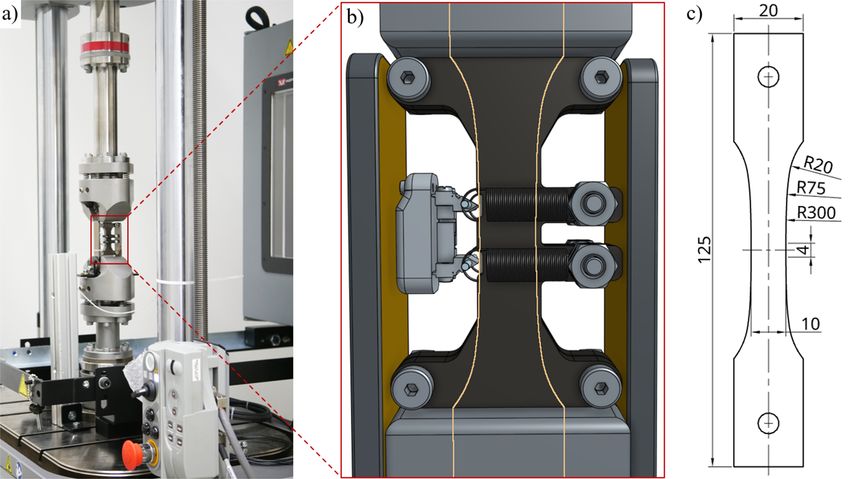
sheets, an anti-buckling device is necessary to
avoid buckling of the specimen and for proper ex-
tensometer mounting, Figure 8a. Tests are per-
formed with five different strain amplitudes ea be-
tween 0.2 % and 0.6 %. Despite using an anti-
buckling device, the testing of high strain ampli-
tudes (ea > 0.6 %) is only possible to a limited ex-
tent, since the results are increasingly influenced by
occurring waviness the higher the compressive
forces get. Therefore, only tests until a strain ampli-
tude of ea = 0.6 % are considered in the present
study.
The two halves of the anti-buckling device are
fastened by four screws to the sample, Figure 8b.
Two vertical guide rails are used to restrict unin-
tended movement of the anti-buckling device dur-
ing the cyclic test. A diamond-like carbon (DLC)
Figure 7. Monotonic tensile stress-strain curve of the stu- coating reduces friction at the sliding contact be-
died electrical steel sheets. tween anti-buckling-device and specimen. Fur-
Bild 7. Monotone Spannungs-Dehnungs-Kurve der unter- thermore, polytetrafluoroethylene-foil is used at the
suchten Elektrobleche unter Zugbeanspruchung. sliding contact between vertical guide rails and
© 2022 The Authors. Materialwissenschaft und Werkstofftechnik published by Wiley-VCH GmbH www.wiley-vch.de/home/muw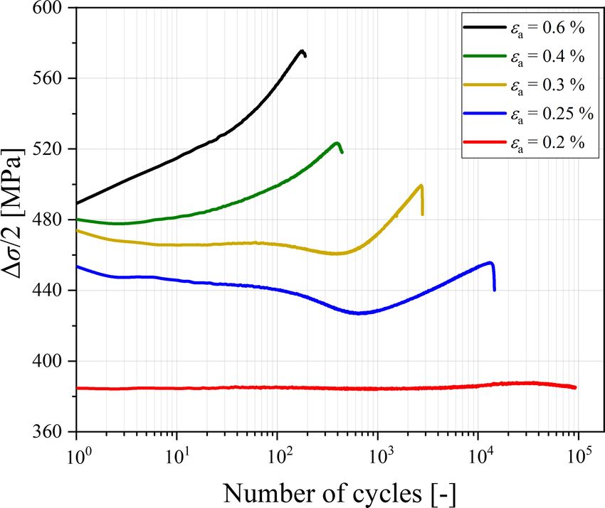
Materialwiss. Werkstofftech. 2022, 53, 422–439                                                       Simulation of thin electrical steel sheets   429

Figure 8. Experimental setup, a) test machine setup, b) detailed view of the anti-buckling device with vertical guide rails,
extensometer, tension springs and specimen, the latter highlighted by a yellow line, c) specimen geometry.
Bild 8. Versuchsaufbau, a) Versuchsmaschinenaufbau, b) Detailansicht der Knickstütze mit vertikalen Führungsschienen,
Extensometer, Zugfedern und Probe, letztere durch eine gelbe Linie hervorgehoben, c) Probengeometrie.

anti-buckling device. A small gap must remain be-                            3.3 Results
tween anti-buckling device and clamping jaws to
avoid buckling and allow unrestricted extension                              The experimental results include representative
and compression of the specimen. Due to the anti-                            stress-strain hysteresis curves at 90 % of fatigue
buckling device, the positioning of the ex-                                  life, Figure 9. Usually, representative hysteresis
tensometer is limited to the small edges of the sam-
ples. By using tension springs for proper mounting,
slippage can be prevented. However, the small con-
tact area between the cutting edge of the ex-
tensometer and the specimen edge can lead to high
local surface pressures. It therefore has to be en-
sured that no crack initiation starting from this con-
tact area is observed.
    Cyclic tests are performed with smooth speci-
mens (Rz < 1.0 μm), which are processed from
sheet material by high precision electrical discharge
machining (EDM). In this study, flat specimens
with 4 mm gauge length and 10 mm width are
used, Figure 8c. The transition area is designed
with three matching radii to achieve a homoge-
neous stress state with a minimised notch factor.

                                                                             Figure 9. Experimental stress-strain hysteresis curves at
                                                                             90 % of fatigue life.
                                                                             Bild 9. Experimentelle Spannungs-Dehnungs-Hysterese-
                                                                             kurven bei 90 % der Ermüdungslebensdauer.

© 2022 The Authors. Materialwissenschaft und Werkstofftechnik published by Wiley-VCH GmbH                          www.wiley-vch.de/home/muw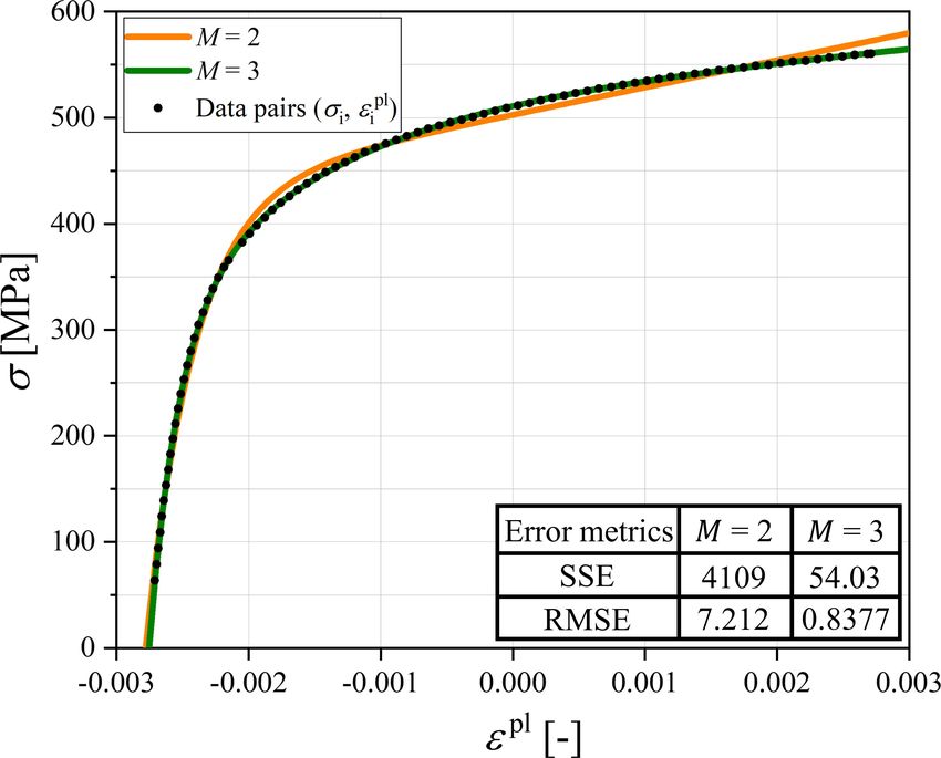
430   P. Kubaschinski                                                                               Materialwiss. Werkstofftech. 2022, 53, 422–439

      curves are defined at 50 % of fatigue life, which is                             haviour is observed at the beginning before rapid
      based on the assumption that the material behaviour                              cyclic hardening occurs.
      has stabilised at half of the number of cycles to                            *   Regarding the lowest strain amplitude
      failure. However, in the case of the studied elec-                               ea = 0.2 %, only slight changes of the stress re-
      trical steel, no stabilised condition is reached dur-                            sponse are observed. No plastic deformation
      ing the cyclic test. Instead, the material exhibits cy-                          takes place, which is why these tests will not be
      clic hardening until crack initiation, Figure 10.                                considered further on.
      Therefore, to describe the material behaviour ap-
      propriately, hysteresis curves are selected at 90 %
      of fatigue life. It is ensured that the chosen stress-                       4 Determination of material parameters:
      strain hysteresis curves do not yet have a crack, as                         material model calibration
      its presence influences the hysteresis shape.
          The extend of cyclic softening/hardening is re-                          4.1 Fundamentals
      vealed by the cyclic accommodation curves consid-
      ering the five different strain amplitudes, Figure 10.                       On the one hand, the material model calibration in
      In general, a division into three material responses                         Abaqus includes the definition of the elastic proper-
      can be made depending on the strain hardening be-                            ties described by Young’s modulus E and Pois-
      haviour:                                                                     son’s ratio n according to the results of the mono-
      * For tests performed at high strain amplitudes                              tonic uniaxial tensile tests, Table 1. On the other
         (ea = 0.4 %, and ea = 0.6 %), the material ex-                            hand, the combined isotropic-kinematic hardening
         hibits substantial cyclic hardening without                               parameters describing the plastic material behav-
         stabilisation until fracture. The stress ampli-                           iour must be calibrated based on the conducted
         tude rises to values slightly higher than the                             symmetric strain-controlled cyclic tests.
         ultimate tensile strength measured in the ten-                                The kinematic hardening parameters can be de-
         sile tests.                                                               termined by the stabilised stress-strain hysteresis
      * For     tests performed at strain amplitudes                               curve, Figure 11a [1, 7]. This usually provides ac-
         ea = 0.25 % and ea = 0.3 % a slight softening be-                         curate results for the considered strain range Δe, as
                                                                                   long as the hysteresis curves are not expected to
                                                                                   significantly differ in shape for varying strains. The
                                                                                   isotropic hardening parameters are determined us-
                                                                                   ing the sequence of the stress-strain hysteresis
                                                                                   curves of a complete cyclic test, Figure 11b.
                                                                                       It has to be considered that the experimental test
                                                                                   data is described in terms of nominal stress snom
                                                                                   and engineering strain enom . Since the material
                                                                                   model calibration in Abaqus requires the true stress
                                                                                   and logarithmic strain as input data, the following
                                                                                   relations are used to convert into the respective
                                                                                   quantities:

                                                                                    s ¼ snom ð1 þ enom Þ                                    (12)
                                                                                    e ¼ lnð1 þ enom Þ                                       (13)

      Figure 10. Cyclic deformation behaviour of the studied
      electrical steel sheets showing continuous cyclic hardening
      without saturation until failure.                                            4.2 Kinematic hardening component
      Bild 10. Wechselverformungsverhalten der untersuchten
      Elektrobleche zeigt kontinuierliche zyklische Verfestigung                   The parameter set of the kinematic hardening com-
      ohne Stabilisierung bis zum Versagen.                                        ponent (Ci , gi ) can be obtained by fitting equa-

      © 2022 The Authors. Materialwissenschaft und Werkstofftechnik published by Wiley-VCH GmbH                          www.wiley-vch.de/home/muw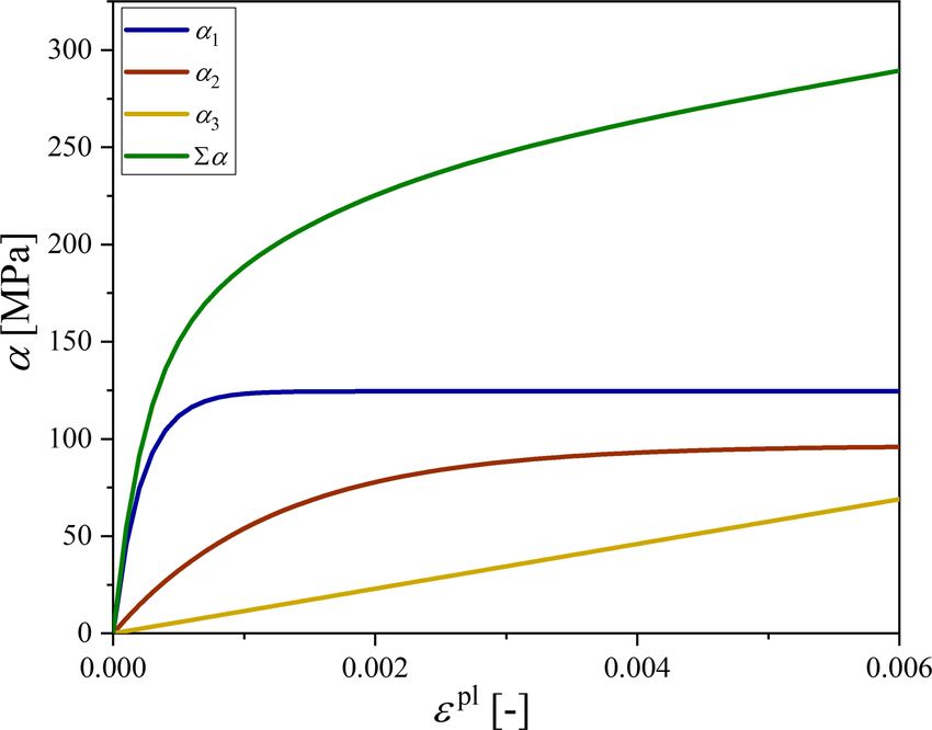
Materialwiss. Werkstofftech. 2022, 53, 422–439                                                       Simulation of thin electrical steel sheets   431

Figure 11. Quantities of the stress-strain hysteresis curves for the determination of a) kinematic hardening, b) isotropic har-
dening [7].
Bild 11. Größen der Spannungs-Dehnungs-Hysterese-Kurven zur Bestimmung von a) kinematischer Verfestigung, b) isotro-
per Verfestigung [7].

                                                                                            si
tion (9) to data pairs (s i ,epl
                              i ) of the stabilised stress-                   epl
                                                                               i ¼ ei                                                    (14)
                                                                                            E
strain hysteresis curve [1]. The calibration can be
performed using the Abaqus internal fitting routine
as well as a nonlinear least-squares regression anal-                           The least-squares regression is performed for
ysis. The stabilised stress-strain hysteresis curve                          two and three back stress components ai , re-
generally shows an initial steep slope followed by a                         spectively. It can be recognised that the quality of
curved section leading to a flatter region [14]. The                         the fit is considerably improved if three back stress
data points of the steep sloped region have a more                           components are used, Figure 12. The root mean
significant influence on the residuals compared to
the flatter region. As a result, less weighting is giv-
en to the flatter region during the curve fitting proc-
ess. At the same time, more weighting is given to
parts of the curve where data points are more con-
centrated. Since Abaqus’ internal fitting routine
does not provide sufficient options to monitor the
quality of the fit, the least-squares regression
should be performed in an external program. In this
paper, the curve fitting toolbox of Matlab is used.
     Stabilised stress-strain hysteresis curves at 90 %
of fatigue life are available for different strain am-
plitudes, Figure 9. In order to determine representa-
tive parameters, the stabilised hysteresis with the
largest strain amplitude (ea = 0.6 %) should be con-
sidered. Thus, it can be ensured that the parameters
are best suitable for a preferably broad strain range
Δe. The start and end values epl         pl
                                    1 , en of the prepared
                                                                             Figure 12. Results of the least-squares regression analysis
                   pl                                                        for the determination of the kinematic hardening component
data pairs (s i ,ei ) correspond to the plastic strain                       considering two and three back stress components.
amplitude �epl;a , Figure 11a. Plastic strain values                         Bild 12. Ergebnisse der Kleinste-Quadrate-Regressions-
epl
  i are calculated by subtracting the elastic from the                       analyse zur Bestimmung der kinematischen Verfestigungs-
total strain ei using the Young’s modulus of the sta-                        komponente unter Berücksichtigung von zwei und drei
bilised cycle:                                                               Rückspannungskomponenten.

© 2022 The Authors. Materialwissenschaft und Werkstofftechnik published by Wiley-VCH GmbH                          www.wiley-vch.de/home/muw
432 P. Kubaschinski Materialwiss. Werkstofftech. 2022, 53, 422–439
squared error (RMSE) is reduced from a value of a function of the equivalent plastic strain �epl [7].
7.2 to 0.84 indicating a reliable fitting result. Both Data pairs (s0i , �epl
i ) should be provided for a range
the data points of the steep sloped as well as the of equivalent plastic strain which is of interest for
flatter region of the curve are accurately captured. the simulation. This usually refers to the condition
The addition of further back stress components is until stabilisation of the hysteresis curves occurs.
not useful, since only minor adjustments can be ex- As mentioned before, electrical steel continuously
pected. With the resulting parameter set, the evolu- exhibits cyclic hardening. The equivalent stress s 0
tion of kinematic hardening is defined, Table 2. For defining the size of the yield surface should there-
its graphical representation, the respective back fore be calibrated until 90 % of fatigue life. At zero
stress components are plotted according to equa- equivalent plastic strain, the initial yield surface
tion (4) under consideration of zero initial plastic size sj0 is defined as the material’s yield strength.
strain and back stress, Figure 13. With the peak tensile stress sti and the maximum
compression stress sci in the elastic range, the yield
surface size of the ith cycle can be calculated, Fig-
4.3 Isotropic hardening component ure 11b:
The isotropic hardening component is determined sti sci
by calculating the equivalent stress s0 , which de- s0i ¼ (15)
2
fines the size of the yield surface (elastic range) as
The corresponding equivalent plastic strain can
be expressed as a function of the cycle number and
Table 2. Resulting kinematic hardening parameters of the plastic strain range Δepl which can be approx-
the three back stress components.
imately calculated with the Young’s modulus E
Tabelle 2. Resultierende kinematische Verfestigungspa- and the peak tensile stress of the first cycle st1 . Us-
rameter der drei Rückspannungskomponenten.
ing the following relations, both quantities can be
C1 g1 C2 g2 C3 g3 assessed [7]:
[MPa] – [MPa] – [MPa] –
2s t1
568467 4566 79017 817.9 11500 0 Depl � De (16)
E
1
�epl
i ¼ ð4i 3ÞDepl (17)
2
The stress-strain hysteresis curves usually show
imperfections [15]. This leads to a deviation from
the shape of an idealised hysteresis curve, Fig-
ure 11. The imperfections include, for example,
strain data slightly exceeding the adjusted strain
range and no sharp corners of the hysteresis curve.
Moreover, the symmetric strain-controlled cyclic
tests of electrical steel sheet specimens are limited
to a relatively small strain range due to buckling
problems. Although the individual deviations are
small, the combined effect of the errors results in
uncertainties [15]. Hence, the identification of the
Figure 13. Evolution of the calculated back stress compo- actual elastic range becomes a quite difficult task,
nents considering zero initial back stress and plastic strain. Figure 14.
Bild 13. Entwicklung der berechneten Rückspannungskom- To allow for an appropriate estimation never-
ponenten unter Berücksichtigung von Null-Anfangsrück- theless, it is proposed to apply a vertical line in the
spannung und plastischer Dehnung. middle area of the rounded corner of the hysteresis
© 2022 The Authors. Materialwissenschaft und Werkstofftechnik published by Wiley-VCH GmbH www.wiley-vch.de/home/muwMaterialwiss. Werkstofftech. 2022, 53, 422–439 Simulation of thin electrical steel sheets 433
Figure 14. Identification of the elastic range of a stress-strain hysteresis curve deviating from the idealised shape by a)
vertical line, b) 0.02 % offset method according to [15].
Bild 14. Identifizierung des elastischen Bereichs einer Spannungs-Dehnungs-Hysterese-Kurve abweichend von der ideali-
sierten Form durch a) vertikale Linie, b) 0,02 % Offset-Methode nach [15].
curve, Figure 14a. The resulting intersections can
be considered as the peak tensile stress and com-
pressive stress in the elastic range. Alternatively, it
is possible to determine the elastic range by apply-
ing a straight line with the slope of the Young’s
modulus of the respective cycle, Figure 14b. Start-
ing from the upper right corner, the end of the elas-
tic range (maximum compression stress) is reached,
when the hysteresis curve begins to separate to a
certain degree from the straight line. With respect
to the described imperfections of the hysteresis
curves, it is suggested to apply the straight line not
at the point of nominal strain amplitude, but with a
0.02 % offset in the negative strain direction [15].
Both methods cannot avoid the described un-
certainties, especially for small strain amplitudes Figure 15. Evolution of isotropic hardening represented by
below 0.3 %, since the separation of elastic and calculated data pairs (s0i , �epl
i ).
plastic portions becomes increasingly difficult. Bild 15. Entwicklung der isotropen Verfestigung dargestellt
durch berechnete Datenpaare (s 0i , �epl
i ).
However, the approach including the application of
a vertical line is expected to represent the better es-
timation of the elastic range for electrical steel, Fig-
ure 14a. plateau. This corresponds to cyclic softening from
It is important to note that the amount of iso- the initial yield surface size sj0 . After the first load
tropic hardening depends on the magnitude of the reversal, the yield plateau disappears and the yield
equivalent (accumulated) plastic deformation [1, 7]. surface size increases over the number of load cy-
As a result, the data pairs (s 0i , �epl
i ) of the isotropic cles as cyclic hardening occurs, Figure 10.
hardening component have to be individually de- Thus, the evolution law of the yield surface size
termined for the different considered strain ampli- has to account for the monotonic behaviour in the
tudes, Figure 15. It shows that, regardless of the first half cycle (initial cyclic softening) and sub-
strain amplitude, the yield surface size decreases in sequently for the actual cyclic behaviour by using
the first half cycle due to the presence of the yield different slopes. Describing the data pairs (s 0i , �epl
i )
© 2022 The Authors. Materialwissenschaft und Werkstofftechnik published by Wiley-VCH GmbH www.wiley-vch.de/home/muw434 P. Kubaschinski Materialwiss. Werkstofftech. 2022, 53, 422–439
with Voce’s law according to equation (10), two The description of the isotropic hardening com-
sets of parameters (sj0 , Q∞ , b) have to be provided. ponent with Voce’s law results in certain diffi-
The rapid decrease of the yield surface size has to culties. The simultaneous implementation of initial
be expressed with a negative maximum change in cyclic softening and subsequent cyclic hardening
the size of the yield surface Q∞ which equals the requires changing the monotonic to the cyclic pa-
difference between s01 and sj0 . The speed of stabili- rameter set after the first load reversal. This change
sation b can then be determined by least-squares re- can lead to an unintended discontinuity in the
gression analysis. In contrast, the increase of the stress-strain relation and consequently to stability
yield surface size is defined by a positive value of problems in the material model definition in Aba-
Q∞ . The required parameters are obtained by least- qus. Moreover, the exponential decline of the iso-
squares regression using the data between s 01 and tropic hardening component during the initial cyclic
s0n . The determination of both the monotonic and softening causes convergence issues. To prevent
cyclic parameter set is performed for the strain am- such problems, the isotropic hardening component
plitude ea = 0.4 %, Table 3. On this basis, the cor- should be defined using the multilinear approach
responding evolution of the yield surface size can according to equation (11). It enables different
be plotted, Figure 16. slopes in the evolution of the isotropic hardening,
which makes it more flexible than Voce’s ex-
ponential law. With the multilinear approach, the
Table 3. Monotonic and cyclic parameter set of the iso-
tropic hardening evolution for ea = 0.4 % according to Vo-
calculated data pairs (s0i , �epl
i ) are connected assum-
ce’s law. ing a linear relation between them.
Tabelle 3. Monotoner und zyklischer Parametersatz der
The rapid decrease of the yield surface size in
isotropen Verfestigungsentwicklung für ea = 0,4 % nach the first half cycle is only described by the first two
dem Gesetz von Voce. data points (sj0 , 0) and (s 01 , �epl
1 ). To allow for a
more accurate representation of the yield plateau,
Parameter set Monotonic Cyclic
an alternative calibration of the isotropic hardening
sj0 [MPa] 447 256 component is suggested. If�the stress-strain
� relation
of the first half cycle s �epl ¼ s epl and the evo-
Q∞ [MPa] 202 49.56
lution of the kinematic hardening component a are
b[ ] 6613 0.6645 known, equation (7) can be solved for the corre-
sponding evolution of isotropic hardening s0 :
� �
s0 �epl ¼ s �epl a (18)
For this purpose, the monotonic stress-strain re-
lation is experimentally determined under the same
test conditions as for the cyclic tests, Figure 17a. It
has to be considered that the subsequent im-
plementation in Abaqus requires a monotonously
increasing stress-strain relation in the material mod-
el definition in order to prevent convergence issues.
Since the experimental data shows the presence of
an upper and lower yield point, it should be
smoothed for further calculations. In accordance
with equation (5), the data pairs can be described
by means of a least-squares regression analysis us-
ing Prager’s linear hardening rule, Figure 17b.
Figure 16. Evolution of isotropic hardening for ea = 0.4 % The resulting evolution of the isotropic harden-
represented by Voce’s law. ing component s0 is plotted for the first half cycle,
Bild 16. Entwicklung der isotropen Verfestigung für Figure 18. In addition, the evolution of kinematic
ea = 0,4 % dargestellt durch das Voce‘sche Gesetz. hardening a is displayed. It shows that the sum of
© 2022 The Authors. Materialwissenschaft und Werkstofftechnik published by Wiley-VCH GmbH www.wiley-vch.de/home/muwMaterialwiss. Werkstofftech. 2022, 53, 422–439 Simulation of thin electrical steel sheets 435
Figure 17. Monotonic stress-strain relation of the first half cycle, a) experiment, b) described by Prager’s linear hardening
rule.
Bild 17. Monotone Spannungs-Dehnungs-Beziehung des ersten Halbzyklus, a) Versuch, b) beschrieben durch die lineare
Verfestigungsregel von Prager.
yield surface size has to be complemented by the
subsequent cyclic hardening. Therefore, the calcu-
lated data pairs (s0i , �epli ) including values between
the second (s 02 , �epl
2 ) and the last cycle (s 0n , �epl
n ) have
to be considered as well. This is indicated by dash-
ed lines for the different strain amplitudes, Fig-
ure 18. The equivalent plastic strain reached at the
point of the first load reversal corresponds to the
data pair of the first cycle (s01 , �epl 1 ). It can be in-
terpreted as the end of the initial cyclic softening
and the onset of the cyclic hardening. As before,
the initial size of the yield surface sj0 is defined at
zero equivalent plastic strain.
Figure 18. Resulting evolution of isotropic, kinematic and 5 Finite-element model implementation in
combined hardening for the first half cycle including in- Abaqus
dicated onset of cyclic hardening.
Bild 18. Resultierende Entwicklung der isotropen, kinemati-
5.1 Simulation setup
schen und kombinierten Verfestigung für den ersten Halbzy-
klus einschließlich des angedeuteten Beginns der zykli-
schen Verfestigung. After the calibration of kinematic and isotropic
hardening parameters, the material behaviour of
electrical steel can be simulated in Abaqus. The
isotropic and kinematic hardening equals the de- specimen geometry used in this study is analysed in
sired stress-strain-relation of the first half cycle. a two-dimensional static simulation using general-
According to that, the calculation using equa- purpose shell elements of type S4R (four-node
tion (18) can be interpreted� as a decomposition of shell, reduced integration), Figure 19. According to
combined hardening s �epl to determine the de- mesh sensitivity studies, an element size of 1 mm is
crease of the yield surface size until the first load chosen for the upper and lower end of the speci-
reversal. To not only represent the monotonic be- men. In the gauge and transition area, the mesh
haviour in the first half cycle, the evolution of the density is refined using an element size of 0.7 mm.
© 2022 The Authors. Materialwissenschaft und Werkstofftechnik published by Wiley-VCH GmbH www.wiley-vch.de/home/muw436 P. Kubaschinski Materialwiss. Werkstofftech. 2022, 53, 422–439
Figure 19. Two-dimensional model of the electrical steel sheet specimen for the numerical simulation of cyclic loading.
Bild 19. Zweidimensionales Modell der Elektroblechprobe zur numerischen Simulation der zyklischen Beanspruchung.
The boundary conditions correspond to the setup of cycle (s 0n , �epl
n ) selected for the respective strain
the experimental cyclic tests. The uniaxial cyclic range, Figure 18.
load is applied at the upper end of the specimen, If the strain range expected in the simulation dif-
whereas the lower end remains fixed. For stress- fers from those which have been considered for the
controlled loading, the magnitude of the effective calibration of the isotropic hardening component,
force is defined by the nominal cross-section of the no calculated data pairs are available. In this case,
specimen. To enable a strain-controlled simulation, it is possible to estimate the evolution of isotropic
the applied displacement amplitude has to be up- hardening (s02 , �epl 0
epl
2 ) to (s n , �n ) by linear inter-
dated depending on the resulting amount of strain polation for strain ranges that lie between the
[16]. In this study, a Python script is implemented known data pairs. Moreover, the evolution of iso-
to iteratively calculate the displacement amplitude tropic hardening can be extrapolated for expected
corresponding to a constant strain amplitude in the strain ranges exceeding the calibrated data. How-
specimen’s nominal cross-section. ever, the extrapolation should be treated carefully,
In the context of the material model definition, since the evolution of the yield surface size cannot
the kinematic hardening component is directly de- be generalised for significantly smaller or larger
fined by the presented parameters, Table 2. The strain ranges. Instead of extrapolating data pairs,
isotropic hardening component on the other side is the isotropic hardening component can be assumed
defined in two steps. In the first step, it is only de- to be constant after the equivalent plastic strain �epl
1
fined for the monotonic behaviour in the first half is reached. As a result, the initial cyclic softening
cycle � according to equation (18). The relation due to the yield plateau is accounted for, while sub-
s0 �epl is provided in tabular form including data sequent cyclic softening/hardening is neglected.
pairs (s 0 , �epl ) from 0 to 1.5 % equivalent plastic
strain, Figure 18. As mentioned before, Abaqus as-
sumes a linear relation between the individual data 5.2 Results and validation with experimental cyclic
pairs. For an accurate � description of the isotropic tests
0 pl
hardening s �e , a small equivalent plastic strain
increment (e. g., �epl = 1�10 5) should therefore be The comparison between simulation and ex-
considered. perimental data is shown for a symmetric strain-
On this basis, the simulation of the monotonic controlled cyclic loading including the strain ampli-
behaviour is performed by calculating the equiv- tudes considered in the material model calibration,
alent plastic strain �epl1 reached at the point of the Figure 20. For each strain amplitude, the first three
first load reversal. With this information, the iso- cycles are represented. It can be seen that the pre-
tropic hardening component can be subsequently dicted material behaviour is basically in good
updated for the simulation of the complete load se- agreement with the experimental cyclic tests. The
quence. The data pair (s 0 , �epl ), which corresponds yield plateau in the first half cycle as well as the
to the equivalent plastic strain �epl
1 , marks the end of onset of the cyclic behaviour are properly de-
the previously defined monotonic behaviour. Then, scribed. Considering the strain amplitudes
the cyclic behaviour is defined by the calculated ea = 0.3 %, ea = 0.4 % and ea = 0.6 %, the shape
data pairs between the second (s02 , �epl2 ) and the last and width of the stress-strain hysteresis curves are
© 2022 The Authors. Materialwissenschaft und Werkstofftechnik published by Wiley-VCH GmbH www.wiley-vch.de/home/muwMaterialwiss. Werkstofftech. 2022, 53, 422–439 Simulation of thin electrical steel sheets 437
Figure 20. Comparison of simulation and experimental data for symmetric strain-controlled cyclic loading with respect to the
first three cycles.
Bild 20. Vergleich von Simulation und Versuchsdaten für symmetrische dehnungskontrollierte zyklische Belastung in Bezug
auf die ersten drei Zyklen.
accurately predicted. Minor differences can be ex- An explanation for this deviation could be the pre-
plained by the influence of the anti-buckling device viously described time-dependent plastic deforma-
on the load cycles. Especially when the loading di- tion which has a more significant influence on
rection is reversed, friction between specimen and small strain ranges and cannot be accounted for in
anti-buckling device has to be overcome which af- the material model.
fects the stress-strain relation in an irregular way. The results for an unsymmetric stress-controlled
Moreover, the experimentally determined hyste- cyclic loading (s max = 500 MPa, Rs = 0.1) are con-
resis curves exhibit rounded corners as already dis- sidered including the first ten load cycles, Fig-
cussed in the context of imperfect cyclic test data. ure 21. In contrast to a strain-controlled loading
This behaviour seems to be related to time-depend- condition, the strain range is not constant. Apart
ent plastic deformation caused by stress relaxation from this, the strain range reached in the first half
under strain-controlled loading [17]. As a result, the cycle clearly exceeds the calibrated data of the iso-
plastic strain continues to increase even though the tropic hardening component (Δe > 0.6 %). Con-
maximum stress is reached. For the strain ampli- sequently, the evolution of the yield surface size
tude ea = 0.25 %, it becomes apparent that the ex- can only be estimated, as mentioned before. In the
perimental data shows a small amount of plastic de- present case, the isotropic hardening component is
formation, whereas the material’s yield strength is assumed to be constant after the equivalent plastic
not exceeded, Figure 17. The simulation on the oth- strain �epl
1 is reached.
er side predicts linear elastic material behaviour.
© 2022 The Authors. Materialwissenschaft und Werkstofftechnik published by Wiley-VCH GmbH www.wiley-vch.de/home/muw438 P. Kubaschinski Materialwiss. Werkstofftech. 2022, 53, 422–439
matic hardening model according to Lemaitre and
Chaboche. For the calibration, isotropic and kine-
matic hardening material parameters have to be de-
termined based on symmetric strain-controlled cy-
clic tests. Special considerations regarding the test
setup are required to prevent buckling of the
0.27 mm thin steel sheets. Using a coated anti-
buckling device, representative tests can be per-
formed for strain amplitudes until 0.6 %. The cali-
bration of the kinematic hardening component
showed that the back stress a is accurately de-
scribed by a parameter set (Ci , gi ) consisting of
three components.
The isotropic hardening component has to ac-
count for different slopes in the evolution of the
Figure 21. Comparison of simulation and experimental data yield surface size to capture both the monotonic be-
for unsymmetric stress-controlled cyclic loading with respect haviour in the first half cycle and the subsequent
to the first ten cycles. cyclic behaviour. With the proposed multilinear ap-
Bild 21. Vergleich von Simulation und Versuchsdaten für proach, the yield plateau (initial cyclic softening) is
unsymmetrische belastungskontrollierte zyklische Belastung
in Bezug auf die ersten zehn Zyklen.
described as difference between the experimentally
determined stress-strain relation of the first half cy-
cle and the kinematic hardening component. After
The comparison with experimental data shows that, the cyclic hardening is represented by the cal-
that the material behaviour in the first half cycle is culated data pairs (s 0i , �epl
i ) starting from the second
correctly represented, while the ratchet strain is un- cycle.
derestimated. This may be explained by the as- The comparison of numerical simulations with
sumed evolution of the yield surface size. Another cyclic tests under strain-control showed a good
possible reason is that the experimentally de- alignment with respect to the shape of the predicted
termined hysteresis curves exhibit distinct rounded stress-strain hysteresis curves. The yield plateau as
corners which again indicates the presence of time- well as the onset of cyclic hardening can be appro-
dependent plastic deformation. More precisely, this priately captured. However, the influence of time-
is associated with a creep deformation process oc- dependent plastic deformation cannot be considered
curring under stress-control [17]. An explicit sepa- which results in noticeable deviations for small
ration in time-dependent and -independent plastic strain ranges and the underestimation of the ratchet-
deformation proves to be difficult. However, the ting behaviour under stress-control. Based on the
experimental data shows that the location of the presented results, the calibrated combined iso-
maximum stress lies more or less in the middle of tropic-kinematic hardening model can be used in
the rounded corners of the hysteresis curves. If the further works to assess the fatigue life of electrical
plastic strain is reduced by the amount of (time-de- steel sheets under proportional cyclic loading.
pendent) strain occurring after the maximum stress
is reached, the difference between simulated and
measured ratchetting behaviour becomes sig- Acknowledgements
nificantly smaller.
This study was performed as part of the research
project “Schwingfestes Elektroblech” funded by the
6 Conclusion Federal Ministry of Education and Research
(BMBF) and the Audi AG. The present work was
In the present study, the cyclic elastic-plastic mate- developed at the Technische Hochschule Ingolstadt
rial behaviour of thin electrical steel sheets has in cooperation with the Otto-von-Guericke-Uni-
been described with the combined isotropic-kine-
© 2022 The Authors. Materialwissenschaft und Werkstofftechnik published by Wiley-VCH GmbH www.wiley-vch.de/home/muwMaterialwiss. Werkstofftech. 2022, 53, 422–439 Simulation of thin electrical steel sheets 439
versität Magdeburg. Open access funding enabled [8] P.J. Armstrong, C.O. Frederick, CEGB Cent.
and organized by Projekt DEAL. Electr. Gener. Board, Report RD/B/N731,
Berkley, UK, 1966.
[9] W. Prager, J. Appl. Phys. 1949, 20, 235.
7 References [10] J.-L. Chaboche, K. Dang Van, G. Cordier,
presented at 5th Int. Conf. Struct. Mech.
[1] R. Halama, J. Sedlák, M. Šofer, in Numerical React. Technol. Berlin, Germany, 1979, Re-
Modelling, (Ed: P. Miidla), IntechOpen, Lon- port number L11/3, pp. 1–10.
don 2012, pp. 329–354. [11] J.-L. Chaboche, G. Rousselier, J. Pressure
[2] J.S. Novak, D. Benasciutti, F. De Bona, A. Vessel Technol. 1983, 105, 153.
Stanojević, A. DeLuca, Y. Raffaglio, IOP [12] J.-L. Chaboche, Int. J. Plast. 1986, 2, 149.
Conf. Ser.: Mater. Sci. Eng. 2016, 119, [13] E. Voce, Metallurgia 1955, 41, 219.
012020. [14] K.H. Nip, L. Gardner, C.M. Davies, A.Y.
[3] J. Lemaitre, J.-L. Chaboche, Mechanics of Elghazouli, J. Constr. Steel Res. 2010, 66, 96.
Solid Materials, Cambridge University Press, [15] E. Arslan, W. Mack, M. Zigo, G. Kepplinger,
Cambridge 2000. PAMM Proc. Appl. Math. Mech. 2017, 17,
[4] C.I. Zub, A. Stratan, D. Dubina, ITM Web 385.
Conf. 2019, 29, 02011. [16] B. Paygozar, S.A. Dizaji, M.A. Saeimi Sa-
[5] J.S. Novak, F. De Bona, D. Benasciutti, Met- digh, J. Mech. Eng. Sci. (JMES) 2020, 14,
als 2019, 9, 950. 6848.
[6] J.-L. Chaboche, Int. J. Plast. 2008, 24, 1642. [17] H.-J. Christ, Wechselverformung von Metal-
[7] Dassault Systèmes Simulia Corp., Abaqus len: Zyklisches Spannungs-Dehnungs-Verhal-
Documentation 2020: Models for metals sub- ten und Mikrostruktur, Springer, Berlin, Hei-
jected to cyclic loading 2020, Dassault Sys- delberg 1991.
tèmes, France.
Received in final form: February 15th 2022
© 2022 The Authors. Materialwissenschaft und Werkstofftechnik published by Wiley-VCH GmbH www.wiley-vch.de/home/muwYou can also read