Automated retinal boundary segmentation of optical coherence tomography images using an improved Canny operator - Nature
←
→
Page content transcription
If your browser does not render page correctly, please read the page content below
www.nature.com/scientificreports
OPEN Automated retinal boundary
segmentation of optical coherence
tomography images using
an improved Canny operator
Jian Liu1,2, Shixin Yan1, Nan Lu3, Dongni Yang3, Hongyu Lv4, Shuanglian Wang5, Xin Zhu6,
Yuqian Zhao1, Yi Wang1,2, Zhenhe Ma1,2 & Yao Yu1,2*
Retinal segmentation is a prerequisite for quantifying retinal structural features and diagnosing
related ophthalmic diseases. Canny operator is recognized as the best boundary detection operator so
far, and is often used to obtain the initial boundary of the retina in retinal segmentation. However, the
traditional Canny operator is susceptible to vascular shadows, vitreous artifacts, or noise interference
in retinal segmentation, causing serious misdetection or missed detection. This paper proposed an
improved Canny operator for automatic segmentation of retinal boundaries. The improved algorithm
solves the problems of the traditional Canny operator by adding a multi-point boundary search step
on the basis of the original method, and adjusts the convolution kernel. The algorithm was used to
segment the retinal images of healthy subjects and age-related macular degeneration (AMD) patients;
eleven retinal boundaries were identified and compared with the results of manual segmentation by
the ophthalmologists. The average difference between the automatic and manual methods is: 2–6
microns (1–2 pixels) for healthy subjects and 3–10 microns (1–3 pixels) for AMD patients. Qualitative
method is also used to verify the accuracy and stability of the algorithm. The percentage of “perfect
segmentation” and “good segmentation” is 98% in healthy subjects and 94% in AMD patients. This
algorithm can be used alone or in combination with other methods as an initial boundary detection
algorithm. It is easy to understand and improve, and may become a useful tool for analyzing and
diagnosing eye diseases.
The structural features of retina have been shown to be closely related to many ophthalmological diseases. For
example, the thickness of the retina, especially the nerve fiber layer (NFL), has been used to indicate the pro-
gression of glaucoma1. It has been reported that the junction of the Inner segment (IS) and the Outer segment
igmentosa2,3. Quantitative assessment of retinal pigment
junction (OSJ) can facilitate the diagnosis of retinitis p
epithelium (RPE) is also useful in diagnosing some age-related macular degeneration (AMD)4. Thus, quantita-
tive research on the retinal features has clinical value. Optical coherence tomography (OCT), as a noninvasive,
label-free and high-resolution imaging modality, has been proven useful to diagnose various retinal diseases5.
The accurate and reliable segmentation of retinal layers in OCT images is a key step in the quantitative study of
retinal features.
Commercial OCT devices are generally equipped with some kind of image analysis software which is able to
perform retinal segmentation with varying success r ates6. However, the details of their design are u ndisclosed7.
In addition, most methods are designed for specific e quipment8. This makes them difficult to replicate in inde-
pendent studies or to be improved by other scholars. Machine learning approaches, including support vector
machines9, random f orest10, and Bayesian artificial neural n etworks11, are proven to obtain satisfactory solu-
tions in a noisy environment12. However, the huge amount of labeled data used in machine learning is difficult
to obtain. Relying solely on manual segmentation will make this task extremely difficult. Furthermore, manual
1
School of Control Engineering, Northeastern University at Qinhuangdao, Qinhuangdao 066004, China. 2Hebei
Key Laboratory of Micro-Nano Precision Optical Sensing and Measurement Technology, Qinhuangdao 066004,
China. 3Department of Ophthalmology, The First Hospital of Qinhuangdao, Qinhuangdao 066004,
China. 4Department of Ophthalmology, Qinhuangdao Maternal and Child Health Hospital, Qinhuangdao 066004,
China. 5Tangshan Maternal and Children Hospital, Tang shan 063000, China. 6Biomedical Information Engineering
Lab, The University of Aizu, Aizu‑Wakamatsu, Fukushima 9650053, Japan. *email: y.j.yu@outlook.com
Scientific Reports | (2022) 12:1412 | https://doi.org/10.1038/s41598-022-05550-y 1
Vol.:(0123456789)
www.nature.com/scientificreports/
segmentation is greatly affected by changes in observers13. Therefore, the automatic retina segmentation algorithm
based on non-machine learning still has certain practical value. It can be used alone, or it can provide a large
amount of label data for machine learning under human supervision.
Anisotropic filtering seems very promising for improving contrast and boundary detection r ate14, but it also
enhances some vertical boundary caused by vascular shadows. In order to avoid this influence, neighborhood
information is often used by some algorithms. The prerequisite is that the retinal layers tend to be horizontal. So,
A-lines alignment on the OCT images is often required before layer segmentation. Qi Yang et al.15 used a large
size gradient template to incorporate adjacent information and deal with vascular shadow and artifacts. Before
that, the IS/OS boundary was first detected, and then the images were further aligned along the IS/OS boundary.
Garvin et al. proposed a 3D graph search approach, which need to first align all the slices and straightened the
RPE layer16. Zhang et al. proposed a segmentation algorithm based on two-step predenoising filtering, which
can only be executed after A-lines alignment17. However, a number of severe eye diseases (AMD, choroidal
neovascularisation (CNV), glaucoma, etc.) can change the structure of retina and choroid18. In this case, A-lines
alignment cannot be performed. The active contour model is good at finding local optima, but its limitation is that
the algorithm cannot converge to the optimal boundary unless the initial point is close enough19,20. Additionally,
the active contour model as a semi-automatic segmentation algorithm requires too much human involvement.
Apparently, if an algorithm relies on human involvement heavily, it will be difficult to deal with large amounts
of data, and more importantly, its performance is difficult to evaluate objectively. Therefore, the development of
a retinal segmentation algorithm with high accuracy and robustness without human intervention has important
clinical significance.
Among the fully automatic edge detection algorithms, Canny operator is recognized as the best operator so far
and is often used to obtain the initial boundary of the retina in retinal segmentation. Unfortunately, if the Canny
operator is applied to retinal edge detection without any modification, it will face some limitations. First, it is
susceptible to the shadow of blood vessels and detects many borders perpendicular to the retinal layer. Second,
the detected boundary may be discontinuous, especially when there are many blood vessels or the image quality
is not ideal. Additionally, it is sensitive to noise interference and is prone to misdetection or missed detection.
Qi Yang et al. combined Canny edge maps and the axial intensity gradient maps to segment the retinal layer15.
The axial intensity gradient maps provide complementary search guidance where Canny edge information is
missing or weak. The layer boundary is then extracted by a shortest path search applied to the graph using a
dynamic programming algorithm. Although this method can alleviate part of the problem of edge discontinuity,
the vertical boundary caused by blood vessel shadow can only be weakened, but cannot be completely eliminated,
which increases the uncertainty of boundary selection.
In this paper, we proposed an automated retinal layer segmentation algorithm based on improved Canny
operator. This method adds a multi-point boundary search step on the basis of the traditional Canny operator
and adjusts the convolution kernel function. The improved Canny operator has a dramatic improvement in the
extraction of the retinal boundary. To make it easier to understand, we divide the algorithm into three parts: First,
Image enhancement, this section includes image denoising, gradient calculation and non-maximum suppression,
which are similar to but slightly different from the first three steps of Canny operator. Second, boundary search,
multiple gradient peak points are selected as seed points to search the retinal boundaries and superimpose the
obtained boundaries together. The third, Boundary selection, the number of superposed boundaries is converted
into probabilities, and the double threshold method in Canny operator is used to select and connect the edges.
This method can accurately distinguish eleven retinal boundaries without additional intervention such as A-lines
alignment, manual initialization, parameter adjustment or search space restriction. Quantitative and qualitative
methods were used to verify the accuracy and stability of the algorithm. We also compared the proposed method
with a state-of-the-art method using public healthy and AMD eye data sets.
Related work
Various automatic retinal segmentation algorithms have been proposed by previous reports. These algorithms
can be divided into two main categories: data-driven a pproaches21–24 and algorithm-driven a pproaches25–28. The
former mainly refers to methods based on traditional machine learning and deep learning. These methods train
classifiers using large amounts of data set to assign specific categories to each pixel in the retinal images. For
example, support vector m achine9,29,30, random forest10 and convolutional neural n
etwork21,22,31–34. Algorithm-
driven approaches, such as level set, graph theory and dynamic programming, mainly construct mathematical
model of retinal boundary segmentation by capturing the anatomical information and optical characteristics
of the retinal layer.
Novosel et al., developed a loosely coupled level set method to segment retinal layers coupling based on the
order of layers and thickness priors but only eight interfaces were detected in the OCT images from normal
retinas35. Subsequently, they use the same method to segment the diseased retinal layers, but only seven surfaces
were detected36.Wang et al.,37 utilized a fuzzy level set-based method to segment diabetic macular edema images.
Compared with other mathematical models, the graph theory based methods have obvious advantages both
in algorithm performance and algorithm c omplexity38. Chiu et al.13 proposed a Graph theory and Dynamic Pro-
gramming (GTDP) approach for automatic segmentation of seven retinal layers. Two years later, they extended
the GTDP algorithm to the segmentation of retina layer with AMD, taking into account the clinical characteris-
tics of the disease on the basis of the original algorithm, and successfully segmented three boundaries39. Garvin
et al.40 optimized the cost function and proposed a method that can be directly used for retinal layer boundary
segmentation in 3D OCT images. Xiang et al.41 proposed a multi-resolution graph search method to perform
simultaneous layer segmentation and fluid segmentation. Recently, Hussain et al.42 proposed a novel approach to
construct graph models. They first extract candidate boundary pixel groups using Canny edge detection operator,
Scientific Reports | (2022) 12:1412 | https://doi.org/10.1038/s41598-022-05550-y 2
Vol:.(1234567890)
www.nature.com/scientificreports/
Figure 1. Illustration of the position of eleven retinal layers. The figure also indicates the full names,
abbreviations and the optical characteristics of each layer.
and then regarded their endpoints as the nodes of the graph. In 2017, LD Sisternes et al.43 proposed a novel
segmentation method based on iterative adaptation of a weighted median process, in which a three-dimensional
weighting function is defined considering image intensity and gradient properties.
Dynamic programming algorithms, due to their significant advantages in solving optimization strategy
problems, have been widely used in retina segmentation. Koozekanani et al. used a Markov boundary model to
connect the rough edge44. But it is sensitive to noise, so the detected layer boundaries can easily deviate from
the true boundary. Mishra et al.20 presented a promising two-step algorithm based on a kernel optimization
scheme. First, approximate positions of the boundaries were found, and then by using dynamic programming
the boundaries were refined to obtain the ideal segmentation results; however, no quantitative evaluation on a
large data set was given. Stephanie J. et al. proposed an automatic initialization method that bypasses the need for
manual endpoint selection of the dynamic programming algorithm13. Tian et al.45 proposed a shortest path based
graph search method to detect retinal boundaries by searching the shortest path between nodes at both ends.
The time complexity was reduced by the limitation of the search region and down-sampling. In order to prevent
the algorithm from accidentally segmenting other structures in place of the target feature, it is often necessary
to limit the graph to a valid search space that excludes any irrelevant content when using dynamic programming
methods. However, the selection of search space will be adjusted artificially according to actual needs.
Materials and methods
Characteristics and nomenclature of retinal layer. Figure 1 shows a cross sectional OCT image of a
normal retina centered at the macula. The positions, full names and abbreviations of the eleven retinal layers are
marked, and the light and dark characteristics of each retinal layer are also indicated.
Each retinal layer is a biological tissue with a specific thickness; however, this paper aims to identify each
retinal boundary. For convenience, we adopted Luis’s43 naming method. The bottom boundary of each retinal
layer was named with the prefix "o-" plus the abbreviation of the retinal layer. For example, the boundary between
NFL and GCL, we call it o-NFL; the boundary between OPL and ONL, we call it o-OPL, and so on. ILM is a thin
layer, so it is treated as a boundary directly. Among the eleven boundaries in the retinal image, the ones from
dark to bright include: ILM, o-GCL, o-INL, o-ONL, o-IS and o-OS, as shown in Fig. 1, indicated by red arrows;
the borders from bright to dark includes: o-NFL, o-IPL, o-OPL, o-OSJ and o-RPE, indicated by blue arrows.
Improved Canny algorithm. The algorithm in this paper is divided into three parts: (1) Image enhance-
ment, (2) Boundary search, (3) Boundary selection. The schematic of the segmentation steps is shown in Fig. 2.
(1) Image enhancement
This section covers image denoising, gradient calculation, and non-maximum suppression, which are similar
to the first three steps of the Canny operator. First, a 3*3 Gaussian filter template is used for image denoising, and
the filtered image is shown in Fig. 3a. Figure 3b is the boundary detection result obtained by using traditional
canny operator. It can be seen that the detected boundaries are discontinuous and contain a large number of axial
boundaries. In order to mainly highlight the horizontal edge, an axial gradient template is used on the gradient
calculation part. The retinal image contains two types of boundaries, from dark to bright and from bright to
dark. The two types of boundaries are enhanced using the ascending gradient template (4 × 1 template, as show
in Eq. 1) and the descending gradient template respectively (4 × 1 template, as show in Eq. 2).
[−1, − 1, 1, 1]T (1)
[1, 1, − 1, − 1]T (2)
Scientific Reports | (2022) 12:1412 | https://doi.org/10.1038/s41598-022-05550-y 3
Vol.:(0123456789)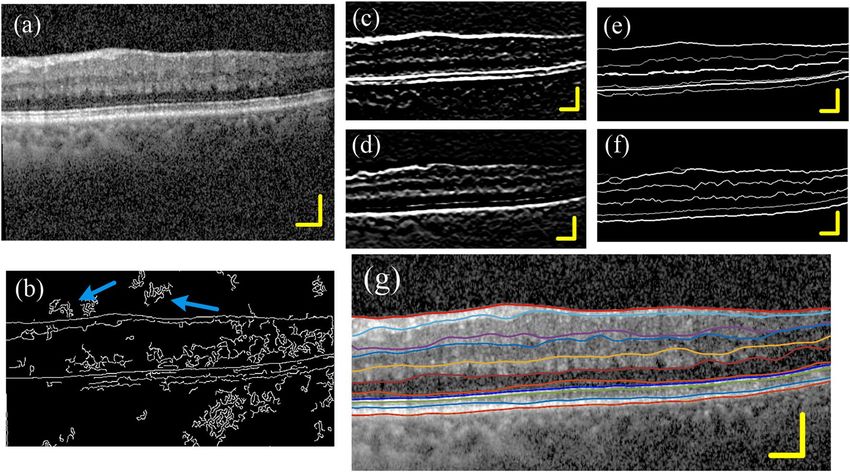
www.nature.com/scientificreports/
Figure 2. Schematic of the segmentation steps.
The 4 × 1 gradient template is more robust than the 2 × 1 gradient template. The gradient image (Fig. 3c) is
obtained by convolving the filtered image with the gradient template (Eq. 1). On the other hand, we perform
large-scale smoothing on Fig. 3a to obtain smooth image (Fig. 3d), the size of the smoothing template is9,10. The
boundary enhancement image (Fig. 3e) is obtained by multiplying the gradient image (Fig. 3c) and the smooth
image (Fig. 3d) point-to-point. The purpose of this step is to weaken the interference outside the retinal image,
such as posterior vitreous face or image noise. Then, the "non-maximum suppression" method is performed
along the A-scan direction to obtain the peak point images (Fig. 3f). These peak points constitute the initial
boundary of the image, but some of these boundaries are discontinuous. Thus, on this basis, we added a multi-
point boundary search method to improve the image boundary. The length of the scale bar in all the pictures
in this article is 200 μm.
(2) Boundary search
Most of the points in Fig. 3f are located at or close to the boundary of the retina. So, these points are used
as seed points to search for retinal boundaries in the gradient image (Fig. 3e). The search criterion is to select
the neighboring point closest to the seed point’s intensity as the potential boundary pixels, and then use this
point as a new seed point to repeat the previous process until it extends to the first or last column of the image.
The search direction can be 3-neighborhoods or 5-neighborhoods, as shown in Fig. 4a,b. 3-neighborhoods are
suitable for Healthy eyes, and 5-neighborhoods are suitable for disease eyes with sharp changes in slope. If two
or more candidate pixels have the same signal intensity, then the algorithm will refer to the extension direction
of the previous step to make a selection. Figure 4c shows a schematic diagram of the extension of a single seed
point. In the end, each seed point will form a path across the B-scan image.
(3) Boundary selection
The boundary path searched by a single seed point may have a certain deviation from the real boundary, but
as the number of paths increases, there will be more and more paths superimposed on the real boundary. We
use Eq. (3) to convert the number of superposed paths into probabilities. Now, the probability value at the real
boundary is much higher than that at other locations.
N
1
(3)
P i, j = · B i, j, n · 100
N
n=1
Finally, the double threshold method in Canny operator was used to filter and connect the paths. Paths with a
probability less than the low threshold are eliminated, and paths with a probability greater than the high threshold
Scientific Reports | (2022) 12:1412 | https://doi.org/10.1038/s41598-022-05550-y 4
Vol:.(1234567890)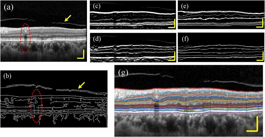
www.nature.com/scientificreports/

                                  Figure 3.  Image edge enhancement. (a) Image after denoising. (b) Boundary detection result obtained by using
                                  traditional canny operator. (c) Gradient image. (d) Large-scale smooth image. (e) Boundary enhanced image. (f)
                                  Peak point image. Scale bar length is 200 μm.

                                  Figure 4.  Three neighborhoods (a) and five neighborhoods (b) boundary search criterion. (c) Boundary search
                                  diagram. The red and blue solid circles represent seed points on different boundaries, and the arrow indicates
                                  the search direction.

Scientific Reports |   (2022) 12:1412 |               https://doi.org/10.1038/s41598-022-05550-y                                               5

                                                                                                                                          Vol.:(0123456789)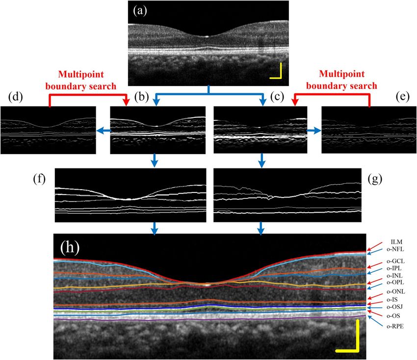
www.nature.com/scientificreports/

                                            Figure 5.  (a) The selection of the seed point area, (b) the obtained retinal boundary image, (c) the gradient
                                            signal and the boundary signal at the position of the blue solid line in (b).

                                            are retained. Then search for points greater than the low threshold at the breakpoints in the high-threshold image,
                                            until the edges of the entire image are closed. Finally, the retinal boundary image was obtained, as show in Fig. 5b.
                                                If all the points in Fig. 3f are used as seed points for boundary search, it will be very time-consuming. In fact,
                                            according to the structural characteristics of the human eye’s macula, it is only necessary to select the seed points
                                            on both sides of the image for calculation, that is, to search the boundary from both sides to the center, and an
                                            ideal result can be obtained. In this paper, 30-pixel-wide local regions on both sides of the image (Fig. 5a color
                                            regions) are selected, and the resulting retinal boundary image is shown in Fig. 5b. Figure 5c shows the gradient
                                            signal and boundary signal at the location shown by the solid blue line in Fig. 5b.

                                            Algorithm entire process and boundary identification. Figure 6 shows the segmentation results of a
                                            normal human retina. Figure 6a is the filtered image. Figure 6b,c are dark-to-bright and bright-to-dark bound-
                                            ary enhancement images, respectively. Figure 6d,e are peak point images after “non-maximum suppression”
                                            processing. Seed points were selected from the peak point images for path search, and the retinal boundary
                                            images were obtained, as shown in Fig. 6f,g. Finally, eleven boundary layers were identified from the two retinal
                                            boundary images in a specific order, as shown in Fig. 6h.
                                                After the boundary image is obtained, eleven retinal boundaries are identified in a certain order. First, the
                                            dark to bright boundaries in Fig. 6f is detected. ILM is defined as the first highlighted reflection layer on each
                                            A-scan in the retinal image, which is most often well demarcated. Next, three outer layer boundaries from dark
                                            to light (o-ONL, o-IS, o-OS) are identified in sequence. Where, the o-IS layer generally has the highest bright-
                                            ness other than the ILM layer in Fig. 6d, so it can be identified in conjunction with Fig. 6d. In Fig. 6f, o-ONL and
                                            o-OS are located above and below the o-IS layer, respectively. ONL is a relatively obvious wide dark band. Above
                                            the o-ONL, the o-INL layer can be detected. Among the dark-to-bright retinal borders, only o-GCL has not yet
                                            been identified. In general, o-GCL is the most unclear layer in the image, so we put it at the end for recognition.
                                                The next step is to determine the bright-to-dark boundaries. o-RPE has the highest brightness in Fig. 6e and
                                            can be identified in conjunction with Fig. 6e. o-OSJ is located between o-IS and o-OS, and the coordinates of
                                            o-OSJ can be restricted between o-IS and o-OS for identification. o-OPL and o-IPL are clearly visible and easy to
                                            identify. o-NFL is the first dark-to-bright interface under ILM. Finally, o-GCL is identified between o-NFL and
                                            o-IPL. All detected boundaries are smoothed using Gaussian filtering, and finally superimposed on the retinal
                                            structure map. The result is shown in Fig. 6h.

                                            Result
                                            Segmentation experiment results.             We recruited 20 subjects (30 eyes), consisting of 10 healthy controls
                                            without ocular or systemic diseases, 10 patients with Mild AMD. Each healthy subject collected images of the left
                                            and right eyes, and AMD patients collected images of the diseased eye on one side. All subjects were recruited
                                            from the First Hospital of Qinhuangdao City. The study was conducted in accordance with the principles of the
                                            Declaration of Helsinki. This study also complies with the ethical guidelines for human medical research and the
                                            quality management norms for drug clinical trials. The research protocol was approved by the ethics committee
                                            of Qinhuangdao First Hospital. Informed consents were obtained from all participants.

          Scientific Reports |   (2022) 12:1412 |                https://doi.org/10.1038/s41598-022-05550-y                                                     6

Vol:.(1234567890)
www.nature.com/scientificreports/

                                  Figure 6.  Segmentation results of the normal human retina. (a) Image after denoising. (b,c) Gradient images.
                                  (d,e) Peak point images. (f,g) Retinal boundary images. (h) Eleven retinal boundaries.

                                      The retinal OCT images used in this study were obtained from a Commercial Spectralis OCT System (based
                                  on Spectralis OCT; Heidelberg Engineering, Heidelberg, Germany). This device operates at 85 kHz A-scan rate,
                                  with a central wavelength of 870 nm and a bandwidth of 50 nm, and provides ~ 3.9-μm axial and 6-μm lateral
                                  resolution. The ocular light power exposure was within the American National Standards Institute safety limit.
                                  Each B-scan datum was composed of 512 A-scans.
                                      Figure 7 shows the segmentation results of a healthy retina and the thickness map of different layers obtained
                                  by the algorithm proposed in this paper. Figure 7a–c are the infrared fundus photography images of healthy eyes.
                                  The green frame is the imaging range of the OCT, and the solid red line points to the current B-scan position.
                                  Figure 7d–f are the retinal images and the layered results at the position shown by the solid red line. Figure 7g
                                  shows the thickness map of the superficial vascular complex (from ILM to o-IPL). Figure 7h is the thickness
                                  map of the deep vascular complex (from o-IPL to o-OPL). Figure 7i is the thickness map of macular inner retinal
                                  layers, which is the sum of Fig. 7g,h. Figure 7j is the thickness map of macular outer retinal layers. The unit of
                                  thickness is μm.
                                      This algorithm is also applicable to the stratification of mild AMD eyes. Figure 8a shows the left eye of a
                                  60-year-old female patient who was diagnosed with wet age-related macular degeneration (wAMD). The best
                                  corrected visual acuity (BCVA) of the left eye was recorded as 20/40. As can be seen from Fig. 8a, the patient is
                                  accompanied by macular edema, subretinal fluid, neuroepithelial and drusenoid pigment epithelial detachments.
                                  Figure 8b is the boundary detection result obtained by using traditional canny operator. Figure 8c,d are dark-to-
                                  bright and bright-to-dark boundaries enhancement image, respectively. Figure 8e,f are retinal boundary images.
                                  Figure 8g is the segmentation results. Figure 8h–j are the thickness maps of superficial vascular complex, deep
                                  vascular complex and macular inner retinal layers, respectively. Figure 8k ~ (m) are the position maps of ILM,
                                  o-IPL and o-OPL. In normal eyes, the center of the macular area is lower than the surrounding area. However,
                                  for AMD eyes with macular edema, the macular fovea area is significantly higher than other surrounding areas.
                                  Therefore, we can see that the middle area in Fig. 8k–m is much higher than the surrounding area.
                                      In the previous section, we show the segmentation results of some undisturbed retinal images. However, in
                                  practical applications, OCT retinal images are often subjected to some interference, such as posterior vitreous
                                  face, vascular artifacts and strong noise interference. Figure 9a is a retinal image with both posterior vitreous

Scientific Reports |   (2022) 12:1412 |                https://doi.org/10.1038/s41598-022-05550-y                                                 7

                                                                                                                                             Vol.:(0123456789)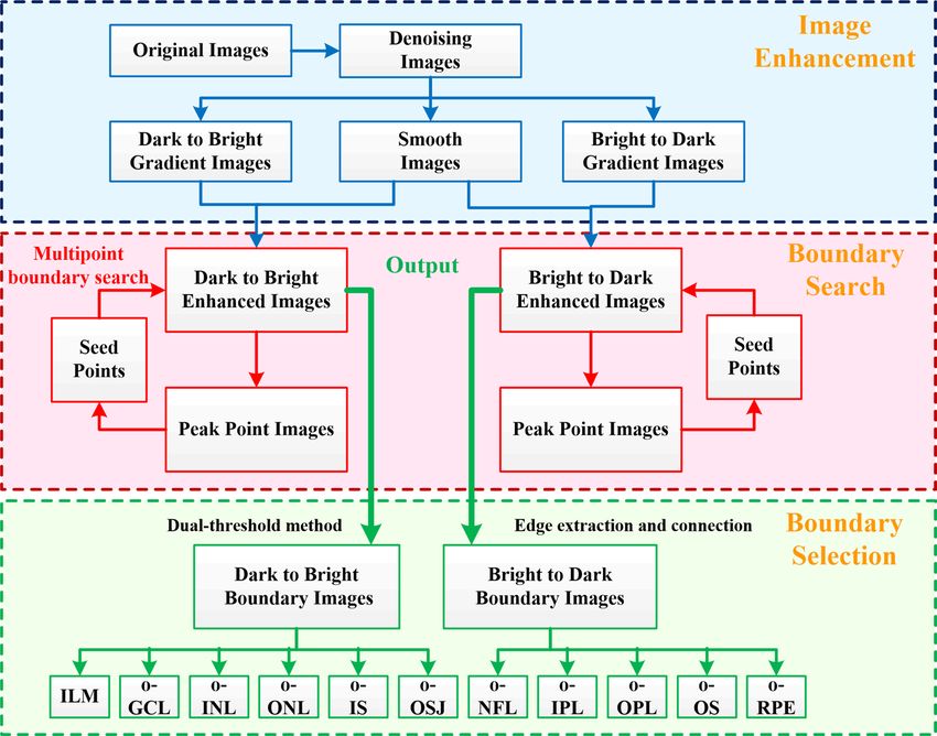
www.nature.com/scientificreports/

                                            Figure 7.  3D segmentation result of a healthy retina and the thickness maps of different layers. (a–c) The
                                            infrared fundus photography images of a healthy eye. The green box is the range of OCT imaging, and the red
                                            solid line points to the current B-scan position. (d–f) The retinal images and the layered results at the position
                                            shown by the solid red line. (g) The thickness map of superficial vascular complex (from ILM to o-IPL). (h) The
                                            thickness map of deep vascular complex (from o-IPL to o-OPL). (i) The thickness maps of macular inner retinal
                                            layers, which are the sum of (g,h). (j) The thickness map of macular outer retinal layers. The unit is μm.

                                            face (yellow arrow) and arterial artifacts (red arrow). Figure 9b is the boundary detection result obtained by
                                            using traditional canny operator. The axial boundary caused by the shadow of the blood vessel is very obvious;
                                            the boundary of the posterior vitreous face is also clearly displayed. Figure 9c–f is the corresponding boundary
                                            detection process using the proposed algorithm. Figure 9g is the final result. Compared with the traditional
                                            canny operator, the algorithm in this paper has a significant improvement in the detection ability of the retinal
                                            boundary.
                                                The quality of OCT images often deteriorates due to the subject’s eye jitter, opacity of the refractive inter-
                                            stitium, or improper operation. It may also be due to the strong speckle noise superimposed on structural images,
                                            which reduces the image contrast near the layer boundaries. Figure 10 shows the segmentation results of a set
                                            of noisy images. It can be seen that the traditional canny operator is very sensitive to noise interference, and the
                                            algorithm in this paper is hardly affected.

                                            Quantitative evaluation. The quantitative evaluation is achieved by comparing the boundary position-
                                            ing difference between the proposed automated method and the manual segmentation method. Among them,
                                            manual segmentation method is implemented by four experienced ophthalmologist using Photoshop software
                                            (Adobe Systems Inc.). They draw 11 retinal boundaries on the B-scan retinal images. The difference in the axial
                                            location of the boundary obtained by the two methods was quantified using the mean unsigned positioning
                                            error (MUE)43. For a particular boundary, the MUE was defined by
                                                                                                      N
                                                                                                  1
                                                                                MUE(L1 , L2 ) =     ·   L1 j − L2 j                                        (4)
                                                                                                  N
                                                                                                       j=1

                                            where L1 and L2 are the results of automatic and manual segmentation of a certain retinal layer, respectively. N
                                            is the number of A-scans included in the B-scan. The eyes of 20 healthy subjects and 10 eyes of AMD patients
                                            were compared and analyzed. The quantitative comparison results are shown in Tables 1 and 2.
                                                We once again averaged the 4 columns of data (mean values) in Tables 1 and 2 to obtain the histogram as
                                            shown in Fig. 11, which can provide a reference for evaluating the accuracy of the proposed algorithm for retinal
                                            segmentation in healthy subjects and AMD patients. The red box in the Fig. 11 represents the average difference
                                            of healthy subjects (the mean of the 4 columns of data in Table 1), and the blue box represents the average differ-
                                            ence of AMD patients (the mean of the 4 columns of data in Table 2), the error bars represent standard deviation.
                                                It can be seen from Fig. 11 that the difference between the automatic and manual segmentation results of the
                                            o-GCL layer of healthy subjects is larger than that of other layers, with an average difference of about 6 microns
                                            (less than 2 pixels). The difference in other layers is about 2–4 microns. The average difference between o-OPL and
                                            o-RPE in AMD patients was significantly larger than that in healthy subjects. The maximum difference is about
                                            10 microns. The increase in the average difference can only explain the difficulty of identifying the boundary and

          Scientific Reports |   (2022) 12:1412 |                https://doi.org/10.1038/s41598-022-05550-y                                                   8

Vol:.(1234567890)
www.nature.com/scientificreports/

                                  Figure 8.  Segmentation result of an AMD eye. (a) A left retina of an AMD patient. (b) Boundary detection
                                  result obtained by using traditional canny operator. (c,d) dark-to-bright and bright-to-dark boundaries
                                  enhanced image. (e,f) retinal boundary images. (g) The segmentation results. (h–j) thickness maps of superficial
                                  vascular complex, deep vascular complex and macular inner retinal layers, respectively. (k–m) position maps of
                                  ILM, o-IPL and o-OPL.

                                  the uncertainty of the segmentation result, but it cannot explain which method is absolutely accurate, because
                                  manual segmentation is not a gold standard either. Therefore, we need to perform further qualitative assessment.

                                  Qualitative evaluation. The qualitative evaluation is achieved by inviting professional readers to score the
                                  automatic segmentation results, with a score ranging from 1 to 4 points. A score of 1 indicates a Perfect or close
                                  to perfect boundary location; a score of 2 indicates a Good boundary location, which may require minor correc-
                                  tions. A score of 3 indicate major problems with boundary location determination and a score of 4 for failing to
                                  produce any result. Each retinal layer is scored separately and the average and standard deviation are calculated
                                  to highlight the algorithm’s ability to recognize different retinal layers. All readers who received the invitation,
                                  whether for quantitative or qualitative evaluation, were senior ophthalmologists from the First Hospital of Qin-
                                  huangdao City. The qualitative evaluation results are shown in Tables 3 and 4.
                                      The 3 columns of data (average values) in Tables 3 and 4 are averaged again to obtain a histogram as shown
                                  in Fig. 12. The red columns represent the average score of healthy subjects (the average of the 3 columns of data
                                  in Table 3), and the blue columns represent the average score of AMD patients (the average of the 3 columns of
                                  data in Table 4), the error bars indicate standard deviation.

Scientific Reports |   (2022) 12:1412 |                https://doi.org/10.1038/s41598-022-05550-y                                                   9

                                                                                                                                               Vol.:(0123456789)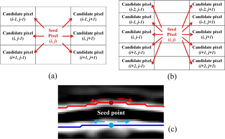
www.nature.com/scientificreports/

                                            Figure 9.  Segmentation results of disturbed image. (a) A retinal image that is disturbed by the posterior
                                            vitreous face. The red ellipse shows a shadow of blood vessel, and the yellow arrow shows the posterior vitreous
                                            face. (b) Boundary detection result obtained by using traditional canny operator. The axial boundary caused by
                                            blood vessel shadows can be seen. (c,d) Dark-to-bright and bright-to-dark boundaries enhanced images. (e,f)
                                            Retinal boundary images. (g) The segmentation results.

                                            Figure 10.  Segmentation results of noisy images. (a) A retinal image of noise interference. (b) Boundary
                                            detection result obtained by using traditional canny operator. The blue arrow indicates a false boundary caused
                                            by noise. (c,d) Dark-to-light and light-to-dark boundaries enhanced image. (e,f) Retinal border images. (g) The
                                            segmentation results.

          Scientific Reports |   (2022) 12:1412 |               https://doi.org/10.1038/s41598-022-05550-y                                                 10

Vol:.(1234567890)
www.nature.com/scientificreports/
Healthy subjects MUE (mean ± SD)
Retinal layer Reader 1 Reader 2 Reader 3 Reader 4
ILM 1.42 ± 1.08 1.66 ± 0.74 1.51 ± 0.57 1.83 ± 0.42
o-NFL 3.06 ± 1.75 3.30 ± 1.25 3.60 ± 1.87 4.32 ± 1.59
o-GCL 4.73 ± 2.71 4.52 ± 2.94 4.96 ± 2.76 7.68 ± 2.34
o-IPL 3.18 ± 1.42 3.45 ± 0.89 3.24 ± 0.95 3.55 ± 1.87
o-INL 2.87 ± 1.73 4.04 ± 1.96 2.59 ± 0.77 3.22 ± 1.71
o-OPL 3.18 ± 1.92 4.28 ± 1.09 3.01 ± 1.27 3.36 ± 2.37
o-ONL 3.02 ± 1.75 2.95 ± 0.84 3.08 ± 0.96 1.91 ± 1.04
o-IS 3.49 ± 1.86 2.63 ± 0.73 3.39 ± 0.97 2.16 ± 1.75
o-OSJ 3.73 ± 1.61 2.95 ± 0.69 3.67 ± 0.57 3.35 ± 2.21
o-OS 4.39 ± 1.87 3.71 ± 1.15 4.69 ± 1.90 3.75 ± 3.37
o-RPE 4.90 ± 2.27 3.17 ± 1.29 5.19 ± 0.94 3.73 ± 1.19
Table 1. Quantitative comparison of boundary positioning between automated and manual segmentation in
healthy subjects’ eyes. MUE mean unsigned positioning error, the unit is μm.
AMD patients MUE (mean ± SD)
Retinal layer Reader 1 Reader 2 Reader 3 Reader 4
ILM 2.14 ± 0.88 2.75 ± 1.23 2.71 ± 1.45 2.77 ± 2.10
o-NFL 3.61 ± 1.10 4.17 ± 2.67 5.76 ± 2.07 4.84 ± 7.14
o-GCL 5.82 ± 1.54 7.60 ± 2.17 7.10 ± 1.80 6.08 ± 6.53
o-IPL 3.49 ± 0.74 4.57 ± 1.16 5.23 ± 1.66 2.73 ± 3.55
o-INL 3.14 ± 0.82 4.19 ± 1.84 4.65 ± 1.52 3.57 ± 1.91
o-OPL 5.09 ± 2.17 6.04 ± 2.86 8.36 ± 3.99 10.1 ± 4.02
o-ONL 4.74 ± 1.53 5.32 ± 1.91 8.18 ± 2.54 5.11 ± 3.56
o-IS 3.96 ± 1.04 4.08 ± 1.74 6.15 ± 2.18 3.77 ± 1.69
o-OSJ 7.17 ± 3.02 4.56 ± 1.25 8.01 ± 5.9 4.69 ± 3.63
o-OS 9.67 ± 3.37 6.13 ± 2.79 10.8 ± 5.9 7.53 ± 6.71
o-RPE 8.11 ± 6.23 6.35 ± 4.59 7.81 ± 6.59 7.86 ± 7.19
Table 2. Quantitative comparison of boundary positioning between automated and manual segmentation in
AMD patients’ eyes. MUE mean unsigned positioning error, the unit is μm.
Figure 11. Average difference between automated and manual segmentation of healthy subjects and AMD
patients.
Scientific Reports | (2022) 12:1412 | https://doi.org/10.1038/s41598-022-05550-y 11
Vol.:(0123456789)www.nature.com/scientificreports/
Healthy subjects score
(mean ± SD)
Retinal layer Reader 1 Reader 2 Reader 3
ILM 1.0 ± 0 1.1 ± 0.31 1.1 ± 0.31
o-NFL 1.2 ± 0.41 1.1 ± 0.31 1.2 ± 0.41
o-GCL 1.6 ± 0.88 1.8 ± 0.42 1.2 ± 0.41
o-IPL 1.1 ± 0.31 1.7 ± 0.48 1.1 ± 0.31
o-INL 1.2 ± 0.41 1.8 ± 0.42 1.3 ± 0.47
o-OPL 1.3 ± 0.47 1.9 ± 0.32 2.2 ± 0.42
o-ONL 1.1 ± 0.31 1.4 ± 0.52 1.0 ± 0
o-IS 1.1 ± 0.31 1.3 ± 0.47 1.0 ± 0
o-OSJ 1.1 ± 0.31 1.1 ± 0.31 1.5 ± 0.53
o-OS 1.2 ± 0.41 1.1 ± 0.31 2.3 ± 0.48
o-RPE 1.1 ± 0.31 1.2 ± 0.41 1.4 ± 0.52
Table 3. Qualitative evaluation in Healthy subjects.
AMD patients score (mean ± SD)
Retinal layer Reader 1 Reader 2 Reader 3
ILM 1.1 ± 0.31 1.1 ± 0.31 1.1 ± 0.31
o-NFL 1.3 ± 0.47 2.2 ± 0.42 1.1 ± 0.31
o-GCL 1.7 ± 0.48 2.8 ± 0.42 1.5 ± 0.53
o-IPL 1.1 ± 0.31 2.2 ± 0.42 1.2 ± 0.41
o-INL 1.2 ± 0.41 2.4 ± 0.52 1.2 ± 0.41
o-OPL 1.4 ± 0.52 2.2 ± 0.42 2.0 ± 0.47
o-ONL 1.1 ± 0.31 1.8 ± 0.42 1.9 ± 0.32
o-IS 1.1 ± 0.31 1.5 ± 0.53 1.5 ± 0.53
o-OSJ 1.3 ± 0.47 1.2 ± 0.41 1.8 ± 0.42
o-OS 2.2 ± 0.42 1.1 ± 0.31 1.3 ± 0.47
o-RPE 1.2 ± 0.41 1.1 ± 0.31 1.2 ± 0.41
Table 4. qualitative evaluation in AMD patients.
Figure 12. Average scores of healthy subjects and AMD patients.
In Fig. 12, the average scores of AMD patients and healthy subjects are very close. It shows that the accuracy
of the segmentation results obtained by the proposed algorithm is very high, and some differences are within
the acceptable or adjustable range.
Comparison with a state‑of‑the‑art method. The proposed method was compared with a state-of-
the-art retinal segmentation method43. We used the same public data set as the literature43, which collected
Scientific Reports | (2022) 12:1412 | https://doi.org/10.1038/s41598-022-05550-y 12
Vol:.(1234567890)www.nature.com/scientificreports/
Figure 13. The segmentation result of public data set obtained by the proposed algorithm. The first row is
b-Scan images of healthy subjects, and the second and third rows are B-scan images of AMD patients.
Proposed method MUE IS-WM43 MUE
Retinal layer Healthy subjects AMD patients All scans Healthy subjects AMD patients All scans
ILM 2.36 ± 1.15 2.88 ± 1.92 2.77 ± 1.75 3.47 ± 4.15 6.43 ± 11.30 5.51 ± 9.76
o-OS 5.35 ± 3.55 8.39 ± 6.81 7.48 ± 6.15 5.41 ± 3.77 7.07 ± 5.66 6.56 ± 5.20
Average 3.86 ± 2.79 5.64 ± 5.72 5.13 ± 5.09 4.44 ± 4.07 6.75 ± 8.93 6.04 ± 7.83
Table 5. Comparison between the proposed method and that in literature43. MUE mean unsigned positioning
error, the unit is μm.
by Farisu et al.46, can be downloaded online. The data set consists of a total of 384 SD-OCT macular scans. Of
these, 115 scans were from healthy subjects, and the remaining 269 scans were from patients with non-exudative
AMD of varying severity. Subjects’ ages and the corresponding manually corrected reference standards for three
retinal layer boundaries are also included. These reference segmentation boundaries were obtained using their
proposed segmentation a lgorithm39 and later corrected manually by experienced graders (certified by the Duke
Advanced Research in Spectral Domain OCT Imaging laboratory): The SD-OCT scans were acquired using
Bioptigen, Inc. (Research Triangle Park, NC) imaging systems at four different clinical sites. Each SD-OCT cube
in the second data set consists of 1000 (horizontal) × 100 (vertical) × 512 (axial) voxels, covering dimensions of
approximately 6.7 (horizontal) × 6.7 (vertical) × 1.6 (axial) mm. In the second data set, the voxel dimensions in
the horizontal, vertical, and axial directions were approximately 6.7, 67, and 3.1-μm respectively.
Figure 13 shows the segmentation results of the public data set obtained by the algorithm in this paper. The
first row shows B-scan images of a typical healthy subject, and the second and third rows show B-scan images
of AMD patients. The first column is the original image, and the second column is the automatic segmentation
result obtained by using the algorithm in this paper. The third column is manually corrected reference standards
boundaries of the ILM, O-OS and O-RPE, which is used to test the accuracy of different methods.
Table 5 shows the comparison results of the algorithm in this paper and the algorithm in literature43. Regard-
ing the identification of the ILM layer, the accuracy of the proposed method is significantly higher than that of
the method in the literature43, both in healthy subjects and AMD patients. For the o-OS layer, the recognition
accuracy of the proposed method is similar to that of healthy people in the literature43, and the recognition accu-
racy of AMD patients is slightly lower. The reason may be that the algorithm in this paper is weak in recognizing
violent fluctuating boundaries, and needs subsequent improvement.
Discussion
Retinal layering algorithms have been developed for many years. The existing methods have one or more of
the following disadvantages: they distinguish only the most prominent layers, they do not exhibit robustness
under noisy and changing conditions, the algorithm is very time-consuming or the algorithm design is very
complicated. Most importantly, most algorithms require more or less human intervention, such as setting the
initial position, setting the search interval, and setting different algorithm parameters or thresholds for different
Scientific Reports | (2022) 12:1412 | https://doi.org/10.1038/s41598-022-05550-y 13
Vol.:(0123456789)www.nature.com/scientificreports/
data sets. These excessive human interventions reduce the objectivity of the algorithm and hinder the use and
development by medical staffs. Therefore, the development of an automatic retinal layering algorithm with high
accuracy and strong anti-interference ability is of great significance for the diagnosis and research of ophthal-
mological diseases.
This paper proposed a retinal layer segmentation algorithm based on improved Canny operator. The con-
ventional canny operator consists of four steps: 1. Image denoising; 2. Gradient calculation; 3. Non-maximum
suppression; 4. Using dual threshold method to select and connect edges. Compared with the traditional canny
operator, the method in this paper has the following improvements:
(1) The traditional canny operator is susceptible to the shadow of the blood vessel, resulting in an edge perpen-
dicular to the retinal layer. This is because the canny operator uses the non-directional Sobel operator as the
convolution kernel function to obtain the image gradient value and gradient direction. It can monitor not
only the horizontal retinal boundary layer, but also the vertical vascular shadow boundary. This paper uses
the axial gradient template to calculate the image gradient, and only horizontal boundary is highlighted.
Additionally, the algorithm uses the method of multiplying gradient images and the large-scale smooth
images to enhance the boundaries of each retina layer, greatly suppressing noise and interference outside
the retina.
(2) Affected by blood vessel shadow or image quality, the boundary detected by the traditional Canny opera-
tor is often discontinuous. In this paper, a multi-point boundary search step is added on the basis of the
traditional canny operator. Several peak points were selected from the non-maximum suppression image as
seed points, and then were extended to both sides in the gradient enhanced image using a boundary search
method to form a path. When encountering the shadow of the blood vessel, the algorithm will continue
the search direction of the previous step and continue to extend forward. In this way, the interference of
blood vessel shadows is well avoided.
(3) The traditional canny operator is sensitive to noise or interference, and is prone to misdetection or missed
detection. In this paper, a certain number of seed points were used to search the boundary together and
the boundaries formed by all the seed points were superimposed on one image. The number of times the
boundary is overlapped is converted into the boundary probability. In general, the real boundaries are
bound to have higher probabilities. Such boundary detection method that relies on the "group effect" can
accurately detect the retinal boundary, even in the case of noise interference, the accurate boundary posi-
tion can be found with a high probability. The use of the dual-threshold method further guarantees the
accuracy and completeness of the boundary. The main advantage of the algorithm is that it almost does not
require any manual involvement (including A-lines alignment, manual initialization, parameter adjustment
or search space restriction, etc.), and its accuracy and stability are also very satisfactory.
In this paper, various types of retinal images are used for testing, and ideal segmentation results were obtained.
This shows that the algorithm has strong accuracy and robustness in dealing with the interference of posterior
vitreous face, blood vessel shadow, noise and lesions. The quantitative and qualitative evaluation results also fully
confirmed this point. From the quantitative evaluation results, the average difference between the automatic seg-
mentation algorithm and the manual segmentation algorithm is: 2–6 microns (1–2 pixels) for healthy subjects,
3–10 microns (1–3 pixels) for patients with mild AMD. From the qualitative evaluation results, the proportion
of scores of 1 or 2 is 98% of healthy subjects and 94% of AMD patients.
The method described in this paper was implemented using MATLAB (The MathWorks, Inc.) M-file code.
The program runs on a personal computer (64 bit OS, Intel Core i7 CPU at 3.6 GHz, and 8 GB RAM) and took
about 124 s to complete the whole 3-D image volume (480 × 512 × 300) pixels detection of eleven layer bounda-
ries. The average processing time for each B-Scan is 242 ms. If a more efficient language was used, for example
C+ programming language, the program can perform with dramatically reduced processing time. If the seg-
mentation process is performed once every 4 B-scans, and then the interpolation method is used to fill the gaps,
then only 128 retinal segmentations need to be performed for 512 B-scans. The time consumed will be reduced
to 1/4 of the original. The processing speed of the proposed method is much higher than that of the method in
reference43 and slightly lower than that of the method in reference47 (the fastest retinal segmentation method to
date). However, the number of retinal layers identified by the proposed method (11 layers) is greater than that
by the method in reference (8 layers)47.
The algorithm currently does not add excessive error correction processing based on prior information.
Therefore, there is still a lot of room for improvement in algorithm performance. It is worth noting that the
method in this paper has a very high accuracy rate for retinal segmentation for patients with mild AMD, but for
severe AMD patients, the recognition accuracy will decrease due to the increase in subretinal fluid and severe
retinal structural deformation. This algorithm can be used alone or in combination with other methods as an
initial boundary detection algorithm to improve the ability to detect AMD retinal boundaries. The proposed
technique can also be extended to segment other hierarchical structures.
In summary, the retinal segmentation algorithm based on the improved Canny operator proposed in this
paper is a robust and automatic algorithm that can distinguish eleven retinal boundaries without human interven-
tion; the segmentation results have high accuracy and stability. The algorithm is easy to understand and improve,
and has the potential to become a powerful tool for analyzing and diagnosing eye diseases.
Received: 31 July 2021; Accepted: 12 January 2022
Scientific Reports | (2022) 12:1412 | https://doi.org/10.1038/s41598-022-05550-y 14
Vol:.(1234567890)www.nature.com/scientificreports/
References
1. Tan, O. et al. Detection of macular ganglion cell loss in glaucoma by Fourier-domain optical coherence tomography. Ophthalmol-
ogy 116(12), 2305.e1-2314.e2 (2009).
2. Lima, L. H. et al. Structural assessment of hyperautofluorescent ring in patients with retinitis pigmentosa. Retina 29(7), 1025–1031
(2009).
3. Hood, D. C. et al. The transition zone between healthy and diseased retina in patients with retinitis pigmentosa. Investig. Ophthal-
mol. Vis. Sci. 52(1), 101–108 (2011).
4. Schlanitz, F. G. et al. Performance of drusen detection by spectral-domain optical coherence tomography. Investig. Ophthalmol.
Vis. 51(12), 6715–6721 (2010).
5. Cabrera DeBuc, D. & Somfai, G. M. Early detection of retinal thickness changes in diabetes using optical coherence tomography.
Med. Sci. Monit. 16(3), MT15–MT21 (2010).
6. Han, I. C. & Jaffe, G. J. Evaluation of artifacts associated with macular spectral-domain optical coherence tomography. Ophthalmol-
ogy 117, 1177–1189 (2010).
7. Lee, S. Y., Stetson, P. F., Ruiz-Garcia, H., Heussen, F. M. & Sadda, S. R. Automated characterization of pigment epithelial detach-
ment by optical coherence tomography. Investig. Ophthalmol. Vis. Sci. 53(1), 164–170 (2012).
8. Matt, G. et al. Comparison of retinal thickness values and segmentation performance of different oct devices in acute branch retinal
vein occlusion. Eye 25(4), 511 (2011).
9. Vermeer, K. A., van der Schoot, J., Lemij, H. G. & de Boer, J. F. Automated segmentation by pixel classification of retinal layers in
ophthalmic OCT images. Biomed. Opt. Express 2(6), 1743–1756 (2011).
10. Lang, A. et al. Retinal layer segmentation of macular OCT images using boundary classification. Biomed. Opt. Express 4(7),
1133–1152 (2013).
11. Somfai, G. M. et al. Automated classifiers for early detection and diagnosis of retinopathy in diabetic eyes. BMC Bioinform. 15(106),
1–10 (2014).
12. Kaji, V., Povazay, B., Hermann, B., Hofer, B. & Drexler, W. Robust segmentation of intraretinal layers in the normal human fovea
using a novel statistical model based on texture and shape analysis. Opt. Express 18(14), 14730–14744 (2010).
13. Chiu, S. J., Xiao, T. L., Nicholas, P., Toth, C. A. & Farsiu, S. Automatic segmentation of seven retinal layers in sdoct images congru-
ent with expert manual segmentation. Opt. Express 18(18), 19413–19428 (2010).
14. Xu, X., Lee, K., Zhang, L., Sonka, M. & Abramoff, M. D. Stratified sampling voxel classification for segmentation of intraretinal
and subretinal fluid in longitudinal clinical OCT data. IEEE Trans. Med. imaging 34(7), 1616–1623 (2015).
15. Yang, Q. et al. Automated layer segmentation of macular oct images using dual-scale gradient information. Opt. Express 18(20),
21293–21307 (2010).
16. Garvin, M. M. K. et al. Intraretinal layer segmentation of macular optical coherence tomography images using optimal 3-D graph
search. IEEE Trans. Med. Imaging 27(10), 1495–1505 (2008).
17. Zhang, X., Yousefi, S., Lin, A. & Wang, R. K. Automated segmentation of intramacular layers in fourier domain optical coherence
tomography structural images from normal subjects. J. Biomed. Opt. 17(4), 046011 (2012).
18. Fabritius, T., Makita, S., Miura, M., Myllylä, R. & Yasuno, Y. Automated segmentation of the macula by optical coherence tomog-
raphy. Opt. Express 17(18), 15659–15669 (2009).
19. Mujat, M. et al. Retinal nerve fiber layer thickness map determined from optical coherence tomography images. Opt. Express
13(23), 9480–9491 (2005).
20. Mishra, A., Wong, A., Bizheva, K. & Clausi, D. A. Intra-retinal layer segmentation in optical coherence tomography images. Opt.
Express 17(26), 23719–23728 (2009).
21. Fang, L. et al. Automatic segmentation of nine retinal layer boundaries in OCT images of non-exudative AMD patients using deep
learning and graph search. Biomed. Opt. Express 8(5), 2732–2744 (2017).
22. Roy, A. G. et al. ReLayNet: retinal layer and fluid segmentation of macular optical coherence tomography using fully convolutional
networks. Biomed. Opt. Express 8(8), 3627–3642 (2017).
23. Xiang, D. et al. Automatic retinal layer segmentation of OCT images with central serous retinopathy. IEEE J. Biomed. Health Inform.
23(1), 283–295 (2019).
24. Liu, X. et al. Automated layer segmentation of retinal optical coherence tomography images using a deep feature enhanced struc-
tured random forests classifier. IEEE J. Biomed. Health Inform. 23(4), 1404–1416 (2019).
25. Kafieh, R., Rabbani, H., Abramoff, M. D. & Sonka, M. Intra-retinal layer segmentation of 3D optical coherence tomography using
coarse grained diffusion map. Med. Image Anal. 17(8), 907–928 (2013).
26. Lee, J. Y. et al. Fully automatic software for retinal thickness in eyes with diabetic macular edema from images acquired by cirrus
and spectralis systems. Investig. Ophthalmol. Vis. Sci. 54(12), 7595–7602 (2013).
27. Dufour, P. A. et al. Graph-based multi-surface segmentation of OCT data using trained hard and soft constraints. IEEE Trans.
Med. Imaging 32(3), 531–543 (2013).
28. Liu, X. et al. Shortest path with backtracking based automatic layer segmentation in pathological retinal optical coherence tomog-
raphy images. Multimed. Tools Appl. 78, 15817–15838 (2019).
29. Hassan, B., Raja, G., Hassan, T. & Akram, M. U. Structure tensor based automated detection of macular edema and central serous
retinopathy using optical coherence tomography images. J. Opt. Soc. Am. A 33(4), 455–463 (2016).
30. Srinivasan, P. P., Heflin, S. J., Izatt, J. A., Arshavsky, V. Y. & Farsiu, S. Automatic segmentation of up to ten layer boundaries in SD-
OCT images of the mouse retina with and without missing layers due to pathology. Biomed. Opt. Express 5(2), 348–365 (2014).
31. Venhuizen, F. G. et al. Robust total retina thickness segmentation in optical coherence tomography images using convolutional
neural networks. Biomed. Opt. Express 8(7), 3292–3316 (2017).
32. Pekala, M. et al. Deep learning based retinal OCT segmentation. Comput. Biol. Med. 114, 103445 (2019).
33. Hamwood, J., Caneiro, D. A., Read, S. A., Vincent, S. J. & Collins, M. J. Effect of patch size and network architecture on a convolu-
tional neural network approach for automatic segmentation of OCT retinal layers. Biomed. Opt. Express 9(7), 3049–3066 (2018).
34. Kugelman, J., Caneiro, D. A., Read, S. A., Vincent, S. J. & Collins, M. J. Automatic segmentation of OCT retinal boundaries using
recurrent neural networks and graph search. Biomed. Opt. Express 9(11), 5759–5777 (2018).
35. Novosel, J. et al. Loosely coupled level sets for simultaneous 3d retinal layer segmentation in optical coherence tomography. Med.
Image Anal. 26(1), 146–158 (2015).
36. Novosel, J., Vermeer, K. A., Jong, J. H. D., Wang, Z. & Vliet, L. J. V. Joint segmentation of retinal layers and focal lesions in 3-d oct
data of topologically disrupted retinas. IEEE Trans. Med. Imaging 36(6), 1276–1286 (2017).
37. Wang, J. et al. Automated volumetric segmentation of retinal fluid on optical coherence tomography. Biomed. Opt. Express 7(4),
1577–1589 (2016).
38. Xiang, D. et al. Automatic segmentation of retinal layer in OCT images with choroidal neovascularization. IEEE Trans. Image
Process. 27(12), 5880–5891 (2018).
39. Chiu, S. J. et al. Validated automatic segmentation of AMD pathology including drusen and geographic atrophy in SD-OCT images.
Investig. Ophthalmol. Vis. Sci. 53(1), 53–61 (2012).
40. Garvin, M. K. et al. Automated 3-D intraretinal layer segmentation of macular spectral-domain optical coherence tomography
images. IEEE Trans. Med. Imaging 28(9), 1436–1447 (2009).
Scientific Reports | (2022) 12:1412 | https://doi.org/10.1038/s41598-022-05550-y 15
Vol.:(0123456789)www.nature.com/scientificreports/
41. Shi, F. et al. Automated 3-d retinal layer segmentation of macular optical coherence tomography images with serous pigment
epithelial detachments. IEEE Trans. Med. Imaging 34(2), 441–452 (2015).
42. Hussain, M. A. et al. Automatic identification of pathology-distorted retinal layer boundaries using SD-OCT imaging. IEEE Trans.
Biomed. Eng. 64(7), 1638–1649 (2017).
43. de Sisternes, L. et al. Automated intraretinal segmentation of SD-OCT images in normal and age-related macular degeneration
eyes. Biomed. Opt. Express 8(3), 1926–1949 (2017).
44. Koozekanani, D., Boyer, K. & Roberts, C. Retinal thickness measurements from optical coherence tomography using a Markov
boundary model. IEEE Trans. Med. Imaging 20(9), 900–916 (2001).
45. Tian, J. et al. Real-time automatic segmentation of optical coherence tomography volume data of the macular region. PLoS ONE
10(8), e0133908 (2015).
46. Farsiu, S. et al. Quantitative classification of eyes with and without intermediate age-related macular degeneration using optical
coherence tomography. Ophthalmology 121(1), 162–172 (2014).
47. Zhang, T. et al. Fast retinal layer segmentation of spectral domain optical coherence tomography images. J. Biomed. Opt. 20(9),
096014 (2015).
Author contributions
Z.M., H.L., X.Z., and S.W. participated in the design; S.Y., N.L. and D.Y. performed experiments; Y.W. and Y.Z.
did bioinformatic analysis; J.L., and Y.Y. wrote the article. All authors approved the final version of the manu-
script for its submission.
Funding
This work was supported in part by National Natural Science Foundation of China (61771119, 61901100 and
62075037), Natural Science Foundation of Hebei Province (H2019501010, F2019501132, E2020501029 and
F2020501040).
Competing interests
The authors declare no competing interests.
Additional information
Supplementary Information The online version contains supplementary material available at https://doi.org/
10.1038/s41598-022-05550-y.
Correspondence and requests for materials should be addressed to Y.Y.
Reprints and permissions information is available at www.nature.com/reprints.
Publisher’s note Springer Nature remains neutral with regard to jurisdictional claims in published maps and
institutional affiliations.
Open Access This article is licensed under a Creative Commons Attribution 4.0 International
License, which permits use, sharing, adaptation, distribution and reproduction in any medium or
format, as long as you give appropriate credit to the original author(s) and the source, provide a link to the
Creative Commons licence, and indicate if changes were made. The images or other third party material in this
article are included in the article’s Creative Commons licence, unless indicated otherwise in a credit line to the
material. If material is not included in the article’s Creative Commons licence and your intended use is not
permitted by statutory regulation or exceeds the permitted use, you will need to obtain permission directly from
the copyright holder. To view a copy of this licence, visit http://creativecommons.org/licenses/by/4.0/.
© The Author(s) 2022
Scientific Reports | (2022) 12:1412 | https://doi.org/10.1038/s41598-022-05550-y 16
Vol:.(1234567890)You can also read