Protein-Protein Docking with Large-Scale Backbone Flexibility Using Coarse-Grained Monte-Carlo Simulations - MDPI
←
→
Page content transcription
If your browser does not render page correctly, please read the page content below
International Journal of
               Molecular Sciences

Article
Protein–Protein Docking with Large-Scale Backbone Flexibility
Using Coarse-Grained Monte-Carlo Simulations
Mateusz Kurcinski *, Sebastian Kmiecik * , Mateusz Zalewski                               and Andrzej Kolinski

                                           Biological and Chemical Research Centre, Faculty of Chemistry, University of Warsaw, 02-089 Warsaw, Poland;
                                           mateusz.zalewski.fuw@gmail.com (M.Z.); kolinski@chem.uw.edu.pl (A.K.)
                                           * Correspondence: mkurc@chem.uw.edu.pl (M.K.); sekmi@chem.uw.edu.pl (S.K.)

                                           Abstract: Most of the protein–protein docking methods treat proteins as almost rigid objects. Only
                                           the side-chains flexibility is usually taken into account. The few approaches enabling docking with a
                                           flexible backbone typically work in two steps, in which the search for protein–protein orientations
                                           and structure flexibility are simulated separately. In this work, we propose a new straightforward
                                           approach for docking sampling. It consists of a single simulation step during which a protein
                                           undergoes large-scale backbone rearrangements, rotations, and translations. Simultaneously, the
                                           other protein exhibits small backbone fluctuations. Such extensive sampling was possible using the
                                           CABS coarse-grained protein model and Replica Exchange Monte Carlo dynamics at a reasonable
                                           computational cost. In our proof-of-concept simulations of 62 protein–protein complexes, we obtained
                                           acceptable quality models for a significant number of cases.

                                    Keywords: protein–protein interactions; protein–protein binding; protein–protein complex; coarse-
Citation: Kurcinski, M.; Kmiecik, S.;      grained modeling; multiscale modeling
Zalewski, M.; Kolinski, A.
Protein–Protein Docking with
Large-Scale Backbone Flexibility
Using Coarse-Grained Monte-Carlo           1. Introduction
Simulations. Int. J. Mol. Sci. 2021, 22,        Protein–protein interactions are fundamental in many biological processes. Their
7341. https://doi.org/10.3390/
                                           structural characterization is one of the biggest challenges of computational biology. A
ijms22147341
                                           variety of docking methods are currently available for structure prediction of protein–
                                           protein complexes [1,2]. They can be divided into free (global) and template-based docking.
Academic Editors: Istvan Simon and
                                           Free (global) docking methods are designed to generate many distinct binding configura-
Csaba Magyar
                                           tions. Template-based methods restrict docking to a binding mode found in a structural
                                           template. As demonstrated in the blind docking challenge, Critical Assessment of Pre-
Received: 19 June 2021
Accepted: 4 July 2021
                                           diction of Interactions (CAPRI), template-based methods generate more accurate results
Published: 8 July 2021
                                           but only if a good quality template exists [1–5]. In some cases lacking useful templates,
                                           free global docking can yield acceptable results. According to recent estimates, the best
Publisher’s Note: MDPI stays neutral
                                           free docking methods find adequate models among the top 10 predictions for around 40%
with regard to jurisdictional claims in
                                           of the targets [1]. The CAPRI analysis also indicates that protein backbone flexibility is a
published maps and institutional affil-    big challenge; protein complexes that undergo substantial conformational changes upon
iations.                                   docking get no successful predictions from any method [3–5].
                                                Presently, most of the free docking methods treat the backbone of input protein struc-
                                           tures as rigid. This approximation reduces the protein–protein docking problem to a 6D
                                           (three rotational and three translational degrees of freedom) search space. Rigid-body
Copyright: © 2021 by the authors.
                                           search for the binding site most often rely on the Fast Fourier Transform [6–8]. Other
Licensee MDPI, Basel, Switzerland.
                                           successful approaches include 3D Zernike descriptor-based docking [9,10] or geometric
This article is an open access article
                                           hashing [11]. These rigid-body methods are often used as a first docking step, followed
distributed under the terms and            by scoring [12–16], using experimental data [17] and/or structural refinement to capture
conditions of the Creative Commons         backbone flexibility [5,18]. Molecular Dynamics is perhaps the most common refinement
Attribution (CC BY) license (https://      strategy, either in classic or enhanced sampling versions [17,19–22]. Other tools use ro-
creativecommons.org/licenses/by/           tamer libraries to address side-chain flexibility [23] and Elastic Network Models (ENMs)
4.0/).                                     for modeling backbone rearrangements [24–28]. Accounting for backbone flexibility in

Int. J. Mol. Sci. 2021, 22, 7341. https://doi.org/10.3390/ijms22147341                                          https://www.mdpi.com/journal/ijms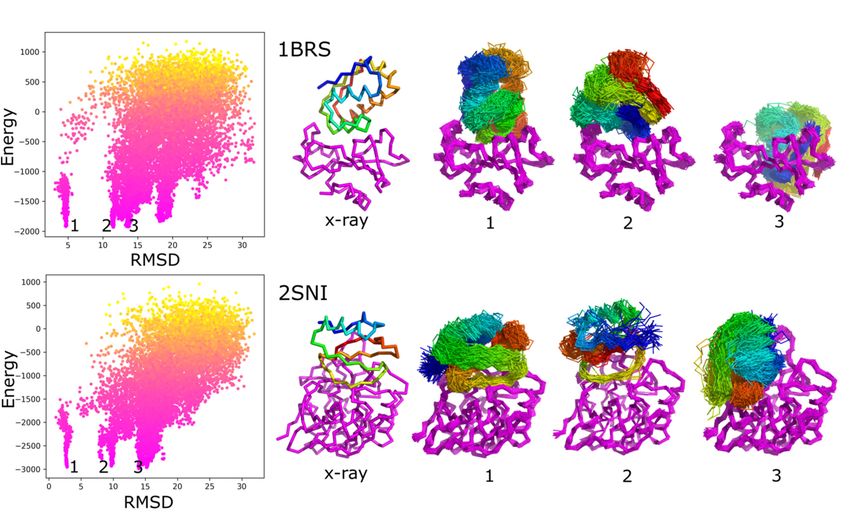
Int. J. Mol. Sci. 2021, 22, 7341                                                                                                       2 of 15

                                       the search for the binding site significantly increases the docking complexity and makes it
                                       practically intractable using conventional all-atom modeling approaches. This enormous
                                       computational complexity of flexible docking can be reduced using coarse-grained protein
                                       models [29–32]. The best-performing methods that can now include backbone flexibility
                                       during the docking calculations use coarse-grained models and/or ENM-driven simu-
                                       lations. These include RosettaDock combining coarse-grained generation of backbone
                                       ensembles and all-atom refinement [33–35]; ATTRACT combining coarse-grained docking
                                       with ENM and all-atom refinement [36,37]; and SwarmDock using all-atom ENM [25,38].
                                       All these approaches show some advantages in modeling protein flexibility compared
                                       to rigid-body docking followed by structure refinements. However, effective modeling
                                       flexibility in protein–protein docking remains an unsolved problem, as demonstrated in
                                       the recent CAPRI round [25,35,37,39].
                                            In this work, we use a well-established CABS coarse-grained protein model [29] for
                                       protein–protein docking. During the CABS docking simulation, one of the docking partners
                                       undergoes a long random process of rotations, translations, and extensive backbone confor-
                                       mational rearrangements that significantly modify its fold. Simultaneously, the backbone
                                       of the second protein undergoes small fluctuations.

                                       2. Results
                                            The most accurate models (out of the sets of 10,000 generated models and 10 top-
                                       scored) are characterized in Table 1. The table presents different metrics of similarity to
                                       the experimental structures for the set of 62 protein–peptide complexes (divided into three
                                       categories: low, medium and high flexibility cases). To assess the sampling performance,
                                       below we will use the iRMSD values for the best models out of all models. According to
                                       the iRMSD values the CABS-based docking algorithm produced a significant number of
                                       near-native protein–protein arrangements of acceptable quality (iRMSD < 4 Å, according
                                       to CAPRI criteria) for most protein–protein cases in the categories of low and medium
                                       flexibility cases. However, in the high-flexibility category, the best iRMSD values were
                                       noticeably higher (in the range of 4–12 Angstroms). This resulted from the adopted distance
                                       restraint scheme (see the Methods section), which was uniform for whole proteins and
                                       introduced a penalty for deviations of more than 1 Å from the input structures (unbound
                                       experimental structures). This penalty was very small for the protein ligands. Thus, the
                                       distance-restraints scheme allowed for the large-scale conformational changes, however,
                                       they might have prevented binding-induced conformational changes in the high-flexibility
                                       category. Therefore, there is the need to modify such a scheme for the most challenging targets.

      Table 1. Summary of the docking simulations. The table characterizes X-ray data used in the docking, average ligand
      flexibility, and docking results. The table reports the best accuracy models out from all (10,000) and 10 top-scored models.
      The metrics definitions are provided in the Methods section. The table divides the presented cases on the three categories:
      low-flexibility, medium-flexibility and highly flexible cases.

                      X-ray Data                                                           Results—Best                 Results—Best
                                                         Ligand Flexibility
                  (Number of Residues)                                                   from All Models          from 10 Top-Scored Models
  Receptor *        Ligand *       Complex   RMSD **     Average LoRMSD        iRMSD        LRMSD      fNAT       iRMSD   LRMSD       fNAT
                                                              Low-flexibility cases
     5CHA            2OVO
                                   1CHO        0.62             4.84              2.65        6.95         0.48    2.96     10.93     0.18
      (238)           (53)
     2PKA             6PTI
                                    2KAI       0.91             4.64              3.32        11.34        0.19    4.75     15.76     0.12
     (232)            (56)
     1CHG            1HPT
                                    1CGI       1.53             5.24              2.76        4.13         0.37    6.18     14.15     0.09
      (245)           (56)
     2PTN             6PTI
                                   2PTC        0.31             5.23              2.97        11.86        0.29    4.39     15.93     0.15
     (223)            (58)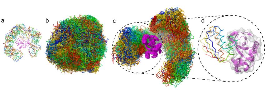
Int. J. Mol. Sci. 2021, 22, 7341                                                                                                    3 of 15

                                                              Table 1. Cont.

                      X-ray Data                                                        Results—Best                 Results—Best
                                                       Ligand Flexibility
                  (Number of Residues)                                                from All Models          from 10 Top-Scored Models
  Receptor *        Ligand *       Complex   RMSD **   Average LoRMSD        iRMSD       LRMSD      fNAT       iRMSD   LRMSD       fNAT
     1SUP             2CI2
                                    2SNI       0.37           3.89             1.09        3.86         0.69    2.81     9.09      0.46
     (275)            (64)
     2ACE             1FSC
                                    1FSS       0.76           4.48             3.41        7.20         0.25   15.03     32.56     0.03
     (532)             (61)
    1MAA              1FSC
                                   1MAH        0.60           4.58             2.49        3.89         0.45   11.25     24.43     0.06
     (533)             (61)
     1A2P             1A19
                                    1BRS       0.47           3.33             1.94        4.19         0.64    4.01     8.74      0.14
     (108)             (89)
     1CCP            1YCC
                                   2PCC        0.39           4.18             3.13        10.19        0.25   11.89     26.68     0.08
     (294)           (103)
     1SUP             3SSI
                                    2SIC       0.39           4.01             4.03        18.96        0.23    4.77     19.40     0.12
     (275)            (107)
     1VFA            1LZA
                                    1VFB       0.59           3.72             4.61        15.07        0.11   17.45     37.15     0.00
     (223)           (129)
     1MLB            1LZA
                                   1MLC        0.85           3.74             2.82        10.47        0.36    8.04     33.09     0.04
     (432)           (129)
                                                          Medium-flexibility cases
     1CHG            1HPT
                                    1CGI       2.02           5.80             2.46        3.21         0.44    5.86     10.72     0.12
      (226)           (56)
     5C2B             4ZAI
                                   5CBA        1.49           4.51             2.48        7.64         0.42    9.34     16.01     0.10
     (241)             (80)
      5P2            1LXD
                                   1LFD        1.79           4.12             2.87        6.76         0.27   12.47     24.24     0.00
     (166)            (87)
     1R6C            2W9R
                                   1R6Q        1.67           9.27             7.95        11.97        0.14   13.71     35.71     0.00
     (142)            (97)
     1JXQ            2OPY
                                   1NW9        1.97           4.09             7.05        8.69         0.23    9.33     17.55     0.00
     (242)           (106)
     1IAS            1D6O
                                    1B6C       1.96           4.65             4.72        10.74        0.14   12.24     23.99     0.00
     (330)           (107)
     5E56             5E03
                                   5E5M        1.56           4.16             3.83        9.09         0.23   10.96     20.00     0.00
     (116)            (113)
     2HRA            2HQT
                                   2HRK        2.03           7.27             3.55        10.17        0.26   10.81     32.54     0.00
      (180)           (115)
     4BLM             4M3J
                                   4M3K        1.77           4.41             4.96        7.41         0.10   13.75     27.11     0.03
     (256)            (116)
     1E78            5VNV
                                   5VNW        1.49           3.81             5.93        22.23        0.10   23.89     70.83     0.00
     (578)            (120)
     3BX8            3OSK
                                    3BX7       1.63           4.63             4.94        17.46        0.28    6.22     20.32     0.12
     (167)           (121)
     6ETL            4POY
                                   4POU        1.83           4.01             2.91        10.16        0.50    6.55     19.65     0.25
     (124)           (121)
     4FUD            5HDO
                                   5HGG        0.84           4.22             3.59        12.52        0.19   13.00     29.3      0.00
     (246)            (126)
     3TGR            3R0M
                                    3RJQ       0.79           4.00             5.32        16.98        0.13   12.77     33.94     0.00
     (346)           (127)
     6EY5            5FWO
                                    6EY6       1.90           3.86             3.83        6.03         0.14   12.89     27.61     0.00
     (585)            (129)
     1SZ7             2BJN
                                   2CFH        1.55           5.13             1.98        4.01         0.71    2.82     5.50      0.63
     (159)            (141)
     3V6F            3KXS
                                    3V6Z       1.83           7.11             6.12        16.68        0.15    6.66     20.06     0.06
     (437)           (142)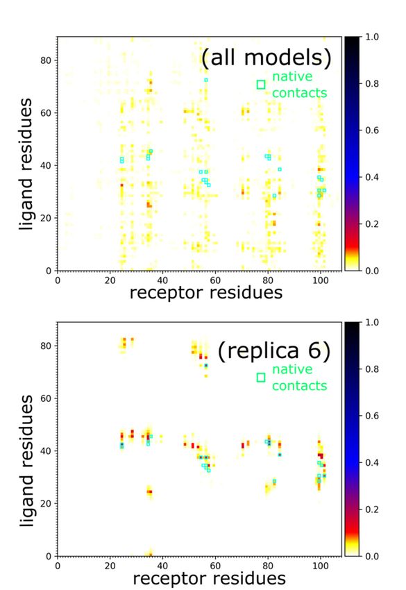
Int. J. Mol. Sci. 2021, 22, 7341                                                                                                     4 of 15

                                                              Table 1. Cont.

                      X-ray Data                                                         Results—Best                 Results—Best
                                                       Ligand Flexibility
                  (Number of Residues)                                                 from All Models          from 10 Top-Scored Models
  Receptor *        Ligand *       Complex   RMSD **   Average LoRMSD        iRMSD        LRMSD      fNAT       iRMSD   LRMSD       fNAT
     3CPI             1G16
                                   3CPH        2.12           4.34             4.87         15.64        0.09   15.02     27.88     0.00
     (437)            (156)
     1QJB            1KUY
                                    1IB1       2.09           4.22             6.56         14.83        0.13   16.10     46.26     0.00
     (460)           (166)
     1IAM            1MQ9
                                   1MQ8        1.76           4.22             4.93         14.99        0.21   26.17     70.50     0.00
     (185)            (173)
     3HI5            1MJN
                                    3HI6       1.65           3.77             5.79         23.30        0.21   19.38     49.77     0.00
     (430)           (179)
     2G75            2GHV
                                   2DD8        2.19           5.37             5.73         13.78        0.09   17.20     34.33     0.00
     (429)            (183)
     1A12            1QG4
                                    1I2M       2.12           4.19             2.84         6.43         0.51    3.58     6.97      0.47
     (401)           (202)
     1N0V             1XK9
                                   1ZM4        2.11           3.54             8.82         28.17        0.04   11.05     48.14     0.00
     (825)            (204)
     4EBQ             4E9O
                                   4ETQ        0.47           3.72             7.12         14.74        0.20    8.68     19.61     0.07
     (429)            (230)
     1S3X            1XQR
                                   1XQS        1.77           5.44             5.63         26.14        0.11   15.88     30.51     0.00
     (380)           (259)
     3HEC            3FYK
                                   2OZA        1.89           4.29             4.35         9.32         0.33   11.24     18.8      0.03
     (329)           (282)
     6A0X             2FK0
                                   6A0Z        1.28           5.75             5.75         25.59        0.16   11.43     31.39     0.00
     (437)            (322)
                                                            Highly flexible cases
     1CL0             2TIR
                                   1F6M        4.9            3.83             7.02         11.34        0.10   11.92     18.06     0.00
     (316)            (108)
    1 × 9Y           1NYC
                                   1PXV        2.63           4.86             5.74         14.10        0.07    7.46     16.31     0.02
     (346)            (110)
     1JZO             1JPE
                                    1JZD       2.71           4.65             4.98         8.13         0.28   13.38     34.05     0.00
     (431)            (116)
     5D7S            2GMF
                                    5C7X       2.26           4.17             4.12         13.61        0.34    4.69     16.74     0.20
     (423)            (121)
     1FCH             1C44
                                    2C0L       2.62           5.51             5.02         5.54         0.21   10.24     24.74     0.00
     (302)            (123)
    1YWH              2I9A
                                    2I9B       3.79           7.14             5.79         17.59        0.14    6.92     33.23     0.05
     (268)            (123)
     3L88            1CKL
                                    3L89       2.51           9.86             4.83         10.90        0.17   17.84     31.87     0.00
     (550)           (126)
     1ZM8              1J57
                                   2O3B        3.13           6.20             4.76         16.43        0.18   15.34     31.95     0.00
     (239)            (143)
     1G0Y             1ILR
                                    1IRA       8.38           4.07             12.97        22.24        0.08   15.86     25.46     0.05
     (310)            (145)
     1QUP            2JCW
                                    1JK9       2.51           9.40             8.07         13.85        0.10   17.41     30.74     0.00
     (219)           (153)
     1SYQ            3MYI
                                   1RKE        4.25           4.15             5.26         6.43         0.38   16.11     34.67     0.00
     (259)           (163)
      2II0           1CTQ
                                   1BKD        2.86           4.51             4.80         7.33         0.14   19.96     39.32     0.00
     (463)           (166)
     1ERN            1BUY
                                    1EER       2.44           5.22             12.97        13.18        0.02   17.12     30.73     0.00
     (416)           (166)
     3AVE            1FNL
                                    1E4K       2.60           5.32             3.44         10.07        0.43    7.59     24.33     0.13
     (419)           (173)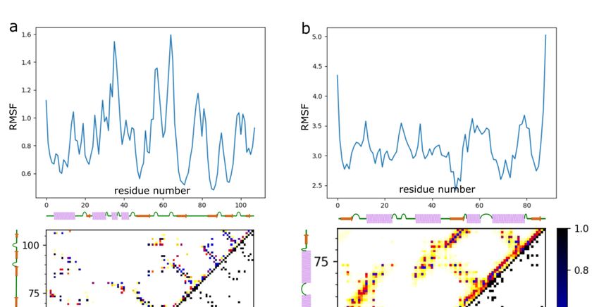
Int. J. Mol. Sci. 2021, 22, x FOR PEER REVIEW 5 of 16
Int. J. Mol. Sci. 2021, 22, 7341 5 of 15
(416) (166)
3AVE 1FNL
1E4K 2.60 5.32
Table 1. Cont.3.44 10.07 0.43 7.59 24.33 0.13
(419) (173)
1R8M 1HUR X-ray Data Results—Best Results—Best
1R8S 3.73 5.50
Ligand Flexibility 6.67 13.41 0.09 15.15 25.10 0.00
(195) (180) of Residues)
(Number from All Models from 10 Top-Scored Models
1QFK *
Receptor 1TFH
Ligand * Complex RMSD ** Average LoRMSD iRMSD LRMSD fNAT iRMSD LRMSD fNAT
1FAK 6.18 5.64 8.97 15.57 0.16 15.59 34.46 0.00
(348)
1R8M (182)
1HUR
1R8S 3.73 5.50 6.67 13.41 0.09 15.15 25.10 0.00
(195) (180)
1F59 1QG4
1QFK 1TFH 1IBR 2.54 5.01 6.65 14.36 0.14 16.41 33.07 0.00
(440) (202) 1FAK 6.18 5.64 8.97 15.57 0.16 15.59 34.46 0.00
(348) (182)
4DVB 4DVA
1F59 1QG4 4DW2
1IBR
2.27
2.54
3.85
5.01
6.61
6.65
21.91
14.36
0.14
0.14
9.94
16.41
29.27
33.07
0.00
0.00
(427)
(440) (246)
(202)
1NG1
4DVB 2IYL
4DVA
2J7P
4DW2 2.67
2.27 4.51
3.85 8.87
6.61 18.77
21.91 0.11
0.14 18.46
9.94 48.05
29.27 0.00
0.00
(294)
(427) (271)
(246)
1UX5
1NG1 2FXU
2IYL
2J7P 2.67 4.51 8.87 18.77 0.11 18.46 48.05 0.00
(294) (271) 1Y64 4.69 4.15 6.42 13.50 0.27 15.50 36.42 0.00
(411) (360)
1UX5 2FXU
1D0N
(411)
1IJJ
(360)
1Y64 4.69 4.15 6.42 13.50 0.27 15.50 36.42 0.00
1H1V 6.62 3.44 7.92 31.14 0.36 29.12 65.07 0.03
(729) (371)
1D0N 1IJJ
* 4-letter PDB
(729) code for1H1V
(371)
6.62
the crystal structures used in3.44 7.92 RMSD31.14
this study. ** The (in Å) of 0.36 29.12Cα atoms
the interface 65.07for input
0.03
receptor and ligand after superposition onto the co-crystallized complex system.
* 4-letter PDB code for the crystal structures used in this study. ** The RMSD (in Å) of the interface Cα atoms for input receptor and ligand
after superposition onto the co-crystallized complex system.
The results analysis below focuses on the sampling performance for the selected
The resultsbarnase/barstar
low-flexibility analysis belowcase.
focuses on the
Figure sampling performance
1 characterizes iRMSD versusfor CABS
the selected
model
low-flexibility
energy values barnase/barstar case. Figure
for the barnase/barstar (1BRS)1and
characterizes iRMSD versus
another low-flexibility CABS
case withmodel
clearly
energy values
the lowest for the
iRMSD barnase/barstar
value (1BRS)
1.09 Angstroms and another low-flexibility case with clearly
(2SNI).
the lowest iRMSD value 1.09 Angstroms (2SNI).
Figure1.1.Characterization
Figure Characterizationofofdocking
dockingresults
resultsusing
usingRMSD
RMSDto tothe
theX-ray
X-raystructure
structureand
andsystem
systemenergy.
energy.The
Theleft
leftpanels
panelsshow
show
the
theinterface-RMSD
interface-RMSDversus CABS
versus CABS energy values.
energy Point
values. color
Point represents
color the temperature—from
represents the temperature—fromyellowyellow
(high)(high)
to pinkto(low).
pink
(low).
The The molecular
molecular visualizations
visualizations showstructures
show X-ray X-ray structures and ensembles
and ensembles of predicted
of predicted models corresponding
models corresponding to selected
to selected energy
energy (numbered
minima minima (numbered in the
in the picture picture
from from
1 to 3). 1 to 3). As
As presented in presented
the picture,inthe
the picture,
minima the minima
numbered as 1stnumbered
corresponds as to
1st
correspondsprotein–protein
near-native to near-native arrangements,
protein–proteinothers
arrangements, others
to non-native to non-native
ensembles, ensembles,
as presented as presented
in the in the
picture. The picture.
presented
ensembles are the sets of similar models found in the structural clustering of contact maps (see Methods). The figure shows
two modeling cases: 1BRS and 2SNI.
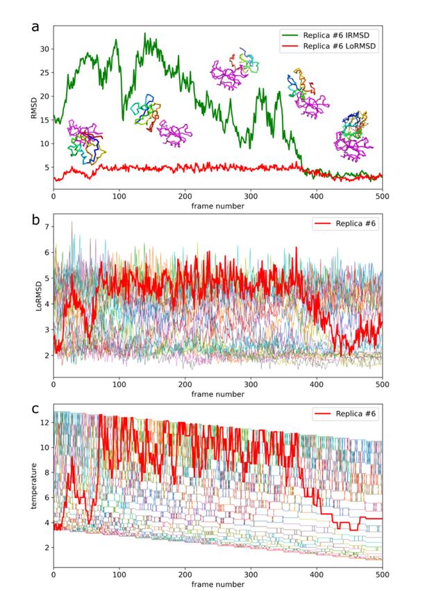
space that involved significantly different binding configurations and protein-ligand
conformations, as demonstrated in Figure 2c and Movie S1. Figure 3a further
characterizes this single replica’s using iRMSD and LoRMSD (RMSD for ligand only)
Int. J. Mol. Sci. 2021, 22, 7341
values. As presented in the figure, the ligand structure fluctuated around 5 Å 6(the of 15
same
fluctuations in the context of all replicas are shown in Figure 3b). The ligand became
significantly more closer to the X-ray structure after binding to the native binding site as
reflected by iRMSD values. Namely, after correct binding, LoRMSD values got noticeably
Figure 2 shows example ensembles of barnase/barstar models and the most accurate
lower to around 2 Å (see Figure 3a). In the following sections, we do not discuss this
model (iRMSD 1.9 Å). A single system replica could explore an ample conformational space
aspect
that of our method;
involved however,
significantly it is binding
different worth mentioning
configurations that
andthe proposed method
protein-ligand enabled
conforma-
a detailed analysis of plausible
tions, as demonstrated in Figure 2cdocking
and Movie trajectories.
S1. Figure 3a The described
further docking
characterizes procedure
this single
uses REMCusing
replica’s protocol
iRMSD enhanced
and LoRMSDby simulated
(RMSD for annealing of all
ligand only) 20 replicas.
values. Figurein3c
As presented theshows
their evolution
figure, the ligandthrough
structuredifferent
fluctuatedtemperatures.
around 5 Å (the Figure
same 4fluctuations
provide morein the detailed
context ofpictures
all
of replicas
structuralare shown in Figure
flexibility 3b). The ligand
for protein became
“receptor” significantly
and “ligand”.more closer to the X-ray
Protein–protein contacts
structure
defining theafter binding
complex to the native
assembly binding site as in
are characterized reflected
Figureby5.iRMSD
In the values.
presentedNamely,
example,
after correct binding, LoRMSD values got noticeably lower to
the most persistent protein–protein contacts occurred in about 15% of snapshots. around 2 Å (see Figure 3a).
In the following sections, we do not discuss this aspect of our method; however, it is worth
Therefore, they were significantly less stable compared to intramolecular protein contacts
mentioning that the proposed method enabled a detailed analysis of plausible docking
(Figure 4).
trajectories. The described docking procedure uses REMC protocol enhanced by simulated
An essential
annealing of all 20 and unique
replicas. feature
Figure of thetheir
3c shows presented
evolutiondocking
through simulations is the level of
different temperatures.
backbone
Figure 4 provide more detailed pictures of structural flexibility for protein “receptor”backbone
flexibility during docking. In the example above, the ligand and
fluctuations (LoRMSD) were
“ligand”. Protein–protein in the range
contacts definingof the
2–7complex
Å (Figure 3b), with
assembly arethe average LoRMSD
characterized in
Figure
value 5. In
of 3.3 Å the
frompresented
the entireexample,
docking the simulations.
most persistent Inprotein–protein
other cases, the contacts
ligandoccurred
fluctuations
in about
were 15% oflevel
at a similar snapshots.
or higherTherefore, they were
(see LoRMSD significantly
values in Tableless
1). stable compared to
intramolecular protein contacts (Figure 4).
Figure 2. Protein–protein docking stages illustrated by barstar/barnase docking case. The figure shows the barnase receptor
Figure 2. Protein–protein docking stages illustrated by barstar/barnase docking case. The figure shows the barnase
in magenta and the barstar ligand in rainbow colors. The respective panels show: (a) 20 starting structures for each replica
receptor in magenta and the barstar ligand in rainbow colors. The respective panels show: (a) 20 starting structures for
of the system; (b) 10,000 models combined from 20 replicas (500 models per replica) in which the highly flexible ligand is
each replica of the system; (b) 10,000 models combined from 20 replicas (500 models per replica) in which the highly
covering the entire surface of the flexible receptor; (c) 500 models from one replica only, (d) the best model obtained for
flexible ligand is covering the entire surface of the flexible receptor; (c) 500 models from one replica only, (d) the best
barnase/barstar system (the X-ray structure of the ligand is shown in thick ribbon, the modeled in thin ribbon).
model obtained for barnase/barstar system (the X-ray structure of the ligand is shown in thick ribbon, the modeled in thin
ribbon). An essential and unique feature of the presented docking simulations is the level of
backbone flexibility during docking. In the example above, the ligand backbone fluctua-
tions (LoRMSD) were in the range of 2–7 Å (Figure 3b), with the average LoRMSD value of
3.3 Å from the entire docking simulations. In other cases, the ligand fluctuations were at a
similar level or higher (see LoRMSD values in Table 1).
Finally, using structural clustering of contact maps (see Methods), we attempted to
select the set of 10 top-scored models for each case. Table 1 reports the most accurate
models out of the 10 top-scored.
Mol. Sci. 2021, 22, x FOR PEER REVIEW

       Int. J. Mol. Sci. 2021, 22, 7341                                                                                                       7 of 15

                                               Figure 3. Docking trajectory for the selected replica of barnase/barstar system. The presented replica
                                          Figure   3. Docking trajectory for the selected replica of barnase/barstar system. The
                                               reached the most accurate barnase/barstar complex structure. (a) iRMSD (interface RMSD) and
                                          replica reached the most accurate barnase/barstar complex structure. (a) iRMSD (interfa
                                               LoRMSD (ligand only RMSD) values. Example simulation snapshots illustrate the plot. The ligand is
                                          and LoRMSD
                                               presented in (ligand       only the
                                                              rainbow colors,   RMSD)
                                                                                    receptorvalues.    Example
                                                                                              in magenta.  The lowestsimulation
                                                                                                                         iRMSD model snapshots
                                                                                                                                       (1.9 A fromillustrate
                                                                                                                                                   X-ray     th
                                          ligand  is  presented       in  rainbow      colors,   the  receptor     in   magenta.     The    lowest
                                               structure) is presented on the right lower corner superimposed on the X-ray structure (the X-ray     iRMSD    mo
                                          fromstructure
                                                X-ray structure)         is presented
                                                         is shown in thick                 on the
                                                                            lines, the predicted    right
                                                                                                 model      lower
                                                                                                        in thin lines).corner    superimposed
                                                                                                                        (b) Ligand                 on the X-ra
                                                                                                                                   only RMSD (LoRMSD)
                                               values  for all replicas. The thick  red line presents selected  replica.  (c) Exchange
                                          (the X-ray structure is shown in thick lines, the predicted model in thin lines). (b) Li     of system replicas
                                               between different temperatures driven by Replica Exchange Monte Carlo (REMC) system. The thick
                                          RMSD    (LoRMSD) values for all replicas. The thick red line presents selected replica. (c) E
                                               red line presents selected replica. The replica trajectory is also presented in the Video S1.
                                          system replicas between different temperatures driven by Replica Exchange Monte Car
                                          system. The thick red line presents selected replica. The replica trajectory is also presen
                                          Video S1.
Int. J. Mol. Sci. 2021, 22, 7341Int. J. Mol. Sci. 2021, 22, x FOR PEER REVIEW 88 of
of1615
Figure 4. Characterization
Figure of barnase/barstar
4. Characterization flexibility in theflexibility
of barnase/barstar docking simulation. The figure
in the docking shows RMSFThe
simulation. plots (uppershows
figure
panels) and contact maps (lower panels) for (a) the barnase receptor and (b) the barstar ligand. The RMSF profile (see
Int. J. Mol. Sci. 2021, 22, x FOR PEER RMSF
REVIEW
Methods) plots
and (upper
contact maps panels)
showing and contact maps
the frequency (lower
of contacts panels)from
are derived for (a)
the9the
of 16 barnase
entire receptor
simulation (derivedand (b) the
from
10,000 models).
barstar ligand. The RMSF profile (see Methods) and contact maps showing the frequency of contacts
are derived from the entire simulation (derived from 10,000 models).
Figure 5. Characterization of barnase/barstar contacts. Panels show barnase/barstar models and
Figure 5. Characterization of barnase/barstar contacts. Panels show barnase/barstar models and
contact maps for entire simulation (all models, 10,000 models) and single selected replica (replica 6,
500contact maps
models) that for aentire
reached simulation
near-native (allInmodels,
arrangement. 10,000
the maps, green models)
circles mark theand single selected replica (replica 6,
native
contacts.
500 models) that reached a near-native arrangement. In the maps, green circles mark the native contacts.
Finally, using structural clustering of contact maps (see Methods), we attempted to
select the set of 10 top-scored models for each case. Table 1 reports the most accurate
models out of the 10 top-scored.
3. Discussion
This work demonstrates a significant improvement in the sampling of large-scale
conformational transitions during global protein–protein docking compared to otherInt. J. Mol. Sci. 2021, 22, 7341 9 of 15
3. Discussion
This work demonstrates a significant improvement in the sampling of large-scale
conformational transitions during global protein–protein docking compared to other state-
of-the-art approaches. We show that modeling the large conformational changes is possible
at a relatively low computational cost. The presented simulations took between 10 and
80 h (depending on the system size) using a single standard CPU. The proposed modeling
protocol can be used as the docking engine in template-based and integrative docking
protocols using experimental structural data and additional information from various
sources [2,40]. We focused on the free docking of protein ligands with a highly flexible
backbone in the present test simulations. Using unbound structures as the input, we
produced acceptable accuracy models (iRMSD around 4 Å or lower) in low-flexibility and
medium-flexibility cases. However, the selection procedure of the most accurate models
needs further improvement. Namely, selecting the best-ranked models led to acceptable
models in about half of the tested cases.
Presently, the most common approach to account for conformational changes in pro-
tein docking is using ENM [24–28,36–38]. The applicability of ENM to modeling protein
flexibility is limited to specific systems and depends on how collective the protein mo-
tions are. Our method presents a conceptually different approach that seems to be more
realistic (see review discussing coarse-grained CABS dynamics in the context of ENM
approaches [24]). We demonstrated that it is possible to simulate effectively free dock-
ing of highly flexible protein ligands to quite elastic protein receptor structures. Such a
significant degree of flexibility was achieved using a highly efficient simulation engine
based on the coarse-grained representation of protein structures, Monte Carlo dynamics,
and knowledge-based force field. CABS coarse-graining, enhanced by the discretized
protein model and interaction patterns, significantly reduces the search space. Monte Carlo
dynamics, enhanced by Replica Exchange annealing, leads to huge speed-up of the search
procedures. Additionally, a significant (although acceptable for many problems) flattening
of energy surfaces by statistical potentials of CABS model simplifies simulations. As a
result the flexible docking using CABS-dock is orders of magnitude faster than equivalent
simulations based on classical modeling methods. Obviously, the new method also has
several limitations that have to be considered when designing new computational experi-
ments. First, since the “ligand” protein is treated as a very elastic object (what is necessary
to guarantee efficient search of the binding sites and poses) the cost of computations rapidly
grows with the protein size. Thus, completely free global docking of protein ligands larger
than 150 residues (see Table 1) may be impractical. Second, the coarse-graining of the
sampling space and simplifying interaction patterns (so important for the huge acceleration
of the simulations) makes the docking energetics less sensitive. For these reasons, the
clustering procedures, refinement of the resulting structures, and final model selection
become challenging and need further development. Additionally, speeding-up the entire
protocol can be useful. We estimate that the simulations could be easily speeded-up at least
10 times or more through algorithm parallelization. The speed-up would enable making
the protocol available as the publicly accessible and automated web service.
4. Methods
4.1. Docking Simulation Protocol
In this work, we present the protein–protein docking simulation protocol that relies
on the CABS coarse-grained model. The CABS design and applications have been recently
described in the reviews on protein coarse-grained [29] and protein flexibility [24,41]
modeling. Here we outline only its main features. The CABS model uses a coarse-grained
representation of protein chains (see Figure 6), Replica Exchange Monte Carlo (REMC)
dynamics, and knowledge-based statistical potentials. Representation of protein chains
is based on C-alpha traces, restricted to an underlying high-resolution lattice. The lattice
spacing allows slight fluctuations of the C-alpha–C-alpha distances and many pseudo-
bonds orientations. Virtual pseudo-atoms are placed in the centers of these C-alpha–C-Int. J. Mol. Sci. 2021, 22, 7341 10 of 15
alpha bonds and are used to locate the main-chain hydrogen bonds. Additionally, the
positions of the two pseudo-atoms representing side chains are defined by the geometry of
C-alpha traces and amino-acid identities. Such fixed positions of side chains (taken from
the statistics of protein databases) reduce the model’s resolution. However, this limitation
is less serious than it may appear since even small movements of the main chain (allowed
due to the soft nature of the assumed geometrical restrictions) leads to large moves11ofofthe
Int. J. Mol. Sci. 2021, 22, x FOR PEER REVIEW 16
side chains. This way, the packing of side chains can be quite accurate. The interaction
scheme of CABS consists of statistical potentials mimicking effects of main chain rotational
preferences, main-chain hydrogen bonds, and side-chain contacts. All statistical potentials,
contacts. All statistical potentials, derived from structural regularities observed in PDB
derived from structural regularities observed in PDB structures, have relatively broad
structures, have relatively broad minima compensating the low-resolution effects and
minima compensating the low-resolution effects and allowing a fast search for global
allowing a fast search for global energy minima. The solvent is treated implicitly, and its
energy minima. The solvent is treated implicitly, and its averaged effects are encoded
averaged effects are encoded within the above-mentioned contact potentials. Energy
within the above-mentioned contact potentials. Energy computation for protein chain
computation
models is very forfast
protein
since chain
many models is very
interactions couldfastbesince many interactions
pre-computed (and codedcould be
in large
pre-computed (anddiscretized
tables) due to the coded in large tables)
patterns duechains
of main to the geometry.
discretizedThepatterns
Monteof main
Carlo chains
sampling
geometry. The Monte Carlo sampling of CABS uses a set of local movers.
of CABS uses a set of local movers. The resulting model dynamics is quite realistic for The resulting
model dynamics
large-scale is quite
distances, realistic
allowing for large-scale
coarse-grained distances,
modeling allowing
of protein coarse-grained
structures, dynamics,
modeling of protein structures,
and protein–protein interactions. dynamics, and protein–protein interactions.
Figure 6. Comparison of the all-atom (left) and the CABS coarse-grained model representation
Figure 6. Comparison of the all-atom (left) and the CABS coarse-grained model representation
(right) for an example tripeptide. In the CABS model, protein residues are represented using C-alpha,
(right) for an example tripeptide. In the CABS model, protein residues are represented using
C-beta, united
C-alpha, C-beta,side-chain atom, and
united side-chain the and
atom, peptide bond center
the peptide bond[29].
center [29].
The modeling protocol consists of the following steps:
The modeling protocol consists of the following steps:
1. Preparing input structures of a protein-ligand and a protein-receptor. The protocol
1. Preparing input structures of a protein-ligand and a protein-receptor. The protocol
requires the input of two protein structures (single- or multi-chain) in the PDB format.
requires the input of two protein structures (single- or multi-chain) in the PDB
One of them has to be indicated as a ligand and the second as a receptor. The ligand
format. One of them has to be indicated as a ligand and the second as a receptor. The
undergoes large conformational fluctuations, translations, and rotations around the
ligand undergoes large conformational fluctuations, translations, and rotations
receptor within the proposed protocol. The “ligand” should be a smaller protein
around the receptor within the proposed protocol. The “ligand” should be a smaller
because the computational cost of searching its conformational space rapidly grows
protein because the computational cost of searching its conformational space rapidly
with the chain length. That is because the motion of the entire structure (including
grows with the chain length. That is because the motion of the entire structure
fold relaxation, rotation, and translation of the entire molecule) is simulated by a
(including fold relaxation, rotation, and translation of the entire molecule) is
random sequence of local moves. The accuracy of such sampling is acceptable for not
simulated
too-large by a random
proteins. sequence
On the of local
other hand, moves.the
treating The accuracy
“ligand” as aoffully
suchflexible
sampling is
object
acceptable for not too-large proteins. On the other hand, treating the
allows approximate studies of entire docking trajectories. In some cases, it would“ligand” as a
fully flexible worth
be perhaps objecttreating
allows aapproximate
larger protein studies of too
(but not entire docking
large) trajectories.
as a flexible In
“ligand”,
some cases, it would be perhaps worth treating
although this was out of range of the present studies.a larger protein (but not too large) as
2. a Generating
flexible “ligand”, although
starting this was
structures. out of
Starting range of the present
conformations are builtstudies.
using C-alpha coor-
2. Generating
dinates onlystarting structures.
(in the CABS modelStarting
C-alphaconformations
traces define theare built using
position of otherC-alpha
united
coordinates only (in the CABS model C-alpha traces define the position of other
united pseudo-atoms, see details [29]). The algorithm places the protein-ligand
center at 20 random positions around the protein receptor at the approximate
distance of 20 Å from the protein receptor’s surface. Next, these protein-ligandInt. J. Mol. Sci. 2021, 22, 7341 11 of 15
pseudo-atoms, see details [29]). The algorithm places the protein-ligand center at
20 random positions around the protein receptor at the approximate distance of 20 Å
from the protein receptor’s surface. Next, these protein-ligand systems are used as
starting conformations for the 20 replicas in the REMC CABS sampling scheme (each
replica starts from a different ligand-receptor arrangement).
3. Docking simulations using CABS coarse-grained model and REMC dynamics. Dur-
ing simulations, the protein receptor structure is kept close to the starting structure
using distance restraints. Distance restraints are generated using the input coordinates
of the C-alpha atoms. Two residues are automatically restrained if two conditions are
met. First, their separation along the sequence has to be at least five residues. Second,
the distance between their C-alpha atoms must be within the range of 5–15 Å. During
simulations, the receptor restraints imply small-scale fluctuations of the protein re-
ceptor backbone in the range of 1 Å and, accordingly, more significant fluctuations
of the side-chain atoms. A similar restraints scheme is applied to the protein-ligand
but with tenfold weaker weights. During simulations, the ligand moves freely within
the vicinity of the receptor and internal restraint allows for large-scale fluctuations of
its structure. Usually, the ligand fluctuations are within the range of 2 and 12 Å to
the input structure although folding-unfolding events are possible at highest temper-
atures. The docking simulation is conducted using CABS REMC pseudo-dynamics
with simulated annealing. In this work, 20 replicas and 20 annealing steps have
been used. All the REMC scheme parameters have been adjusted to allow for large-
scale conformational transitions, rotations, and translations of the protein-ligand in a
reasonable computational time. The modeling protocol collects trajectories from all
20 replicas. The protocol saves only a small fraction (2%) of the generated models for
further analysis i.e., 500 models from each replica, thus 10,000 models in total.
4. Reconstructing to CABS coarse-grained representation. The set of 10,000 models in
C-alpha traces are reconstructed to complete CABS model representation using CABS
algorithm [29]. In CABS, positions of C-beta and Side-Chain united atoms are defined
by the positions of the three consecutive C-alpha atoms and the amino acid identity
(the most probable positions from the PDB database are used).
5. Clustering of contact maps. First, for all of the 10,000 models the contact maps
between the receptor and the ligand proteins are calculated. Two residues are con-
sidered to form a contact if their Side Chain pseudoatoms are at most 6 Å apart (for
Alanines the C-beta atoms are considered as the Side Chain; for Glycines—it’s the
C-alpha atoms). Next, the algorithm sorts the models according to the number of the
receptor-ligand contacts, and the set of top 1000 is kept for further processing. This
way the transient and weakly bound complexes are removed from the solutions pool.
In the next step, the 1000 contact maps are clustered together to identify the most
frequently occurring contact patterns. The complete link hierarchical clustering was
used with the Jaccard index as the distance metric between contact maps. Finally, the
identified clusters are ranked according to their density, defined as the number of the
cluster members divided by the average metric between them.
6. Reconstructing to all-atom representation. Representative models from the ten most
dense clusters are reconstructed to all-atom representation using Modeller-based
rebuilding procedure [42] (or can be reconstructed using other rebuilding strategies,
see review [43]).
In recent years, the CABS model has been used for modeling the flexibility of globular
proteins [44–47] and various processes leading to large-scale conformational transitions.
These included: ab initio simulations of protein folding mechanisms [48,49], folding and
binding mechanisms [49,50], and free protein–peptide docking within the CABS-dock
tool [51–57]. The CABS-dock is a well-established peptide docking tool that has been
made available as a web server [51,52] and, most recently, as a standalone application [54].
Its distinctive feature among other tools is the possibility of fast simulation of the large
backbone rearrangements of both peptide and protein receptors during binding (see theInt. J. Mol. Sci. 2021, 22, 7341 12 of 15
review on protein–peptide docking tools [58]). In addition, the CABS-dock has been used
in multiple applications (recently reviewed [56]), including docking to receptors with
disordered fragments [41,59], GPCRs [60], and modeling proteolysis mechanisms [61].
The presented protocol for protein–protein docking utilizes the CABS-dock standalone
package [54] developed primarily for protein–peptide docking. In order to tackle the
protein–protein docking problem, key changes have been made to the docking algorithm
that aimed mainly at the improvement of the conformational sampling. First of all, the
temperature distribution between replicas in the REMC scheme was adjusted. Instead of
constant temperature increment between consecutive replicas, as in the original CABS-
dock, here we’ve implemented progressive geometric raise of the temperature increment.
Furthermore, the number of simulation replicas was increased to twenty versus ten in the
original CABS-dock. Besides the sampling improvement, a new clustering protocol was
introduced. The original CABS-dock used RMSD-based clustering, which worked well
for peptides. For the protein–protein complexes, however, purely geometrical similarity
condition such as the RMSD is too severe. Namely, for two binding poses, where the mobile
protein was docked in the exact same pocket but is slightly tilted in one of them, the RMSD
difference would be considerable. Despite representing similar binding poses, the two
structures would end up in different clusters. To overcome this, the current protocol uses
clustering based on the similarity between receptor-ligand contact maps.
4.2. Results Analysis and Quality Metrics
The docking simulation analysis was performed using Python and NumPy (Python
library). Structural differences between experimentally determined structures and gen-
erated models were evaluated using Root Mean Square Deviations (RMSDs). Interface
RMSD (iRMSD) is an RMSD calculated for interface residues of the receptor and the ligand
separated by no more than 6 Angstroms. Ligand RMSD (LRMSD) is an RMSD computed
for the ligands after the superimposition of the receptors. Ligand only RMSD (LoRMSD) is
an RMSD computed for the ligand structure only. Root Mean Square Fluctuation (RMSF)
is a measure of the amino acid’s flexibility. It is calculated for every residue as the square
root of this residue’s variance around the reference residue position. The fraction of native
contacts (fNAT) was calculated as a number of experimental structure contacts found in
the generated structure divided by the total number of contacts found in the experimental
structure. Rather restrictive contact criterion, distance up to 6 Å between side-chain centers,
was used. All figures presented in this work were generated using PyMOL, UCSF Chimera,
and Matplotlib (Python library).
4.3. Dataset
In this docking study, we used protein–protein cases from the ZDOCK benchmark
set [62] (cases in which a smaller size protein—a protein-ligand—contained more than one
protein chain, or chain gaps, were discarded from our set). The set comprises the three
flexibility-based subsets: low-flexible (almost rigid), medium-flexible, and highly flexible
with available unbound X-ray structures of both the protein-receptor and the protein-ligand.
The unbound structures were used as the docking input. As the reference for calculating
various similarity measures, we used the X-ray structures of the protein-ligand complexes.
Table 1 lists all the PDB IDs of X-ray structures used in the study.
5. Conclusions
In summary, the described docking procedure accounts for large-scale protein struc-
ture fluctuations during unrestrained protein–protein docking search for the binding site.
The exploration of such vast conformational space has not been demonstrated before to
the best of our knowledge. The approach shows unprecedented sampling possibilities;
however, the accuracy of the obtained complexes is still lower than observed for state-of-
the-art docking tools. Definitely, the balancing of the structural restraints scheme needs
further developments and tests. Therefore, this work is the first step towards a matureInt. J. Mol. Sci. 2021, 22, 7341 13 of 15
protein–protein docking tool. The next development steps would involve modifications of
the distance restraints scheme, which allow for different degrees of flexibility for appropri-
ate protein fragments (now the presented algorithm treats the entire protein-ligand as very
flexible) and force-field improvements. The proposed approach is also very promising in
the refinement applications when searching for the binding site is not needed, and only the
protein–protein interface needs to be optimized.
Supplementary Materials: The following are available online at https://www.mdpi.com/article/
10.3390/ijms22147341/s1, Video S1. The trajectory of a single replica from the protein-protein
docking simulation of barnase/barstar system. The movie shows the barnase receptor in surface
representation and the barstar ligand in ribbon. The presented replica reached the model with
interface RMSD value 1.9 Angstrom from the complex X-ray structure, shown as transparent ribbon.
Author Contributions: Conceptualization, M.K., S.K. and A.K.; Methodology, M.K. and A.K.; Soft-
ware, M.K. and M.Z.; Supervision, S.K.; Visualization, M.K. and S.K.; Writing—original draft, S.K.;
Writing—review & editing, M.K., S.K., M.Z. and A.K. All authors have read and agreed to the
published version of the manuscript.
Funding: SK: MZ and AK acknowledge funding by the National Science Centre, Poland [MAE-
STRO2014/14/A/ST6/00088]. MK acknowledges funding by the National Science Centre, Poland
[501/D112/66 GR-6271]. SK also acknowledges funding in part by the National Science Centre,
Poland [UMO-2020/39/B/NZ2/01301].
Institutional Review Board Statement: Not applicable.
Informed Consent Statement: Not applicable.
Data Availability Statement: Not applicable.
Conflicts of Interest: The authors declare no conflict of interest.
References
1. Porter, K.A.; Desta, I.; Kozakov, D.; Vajda, S. What method to use for protein–protein docking? Curr. Opin. Struct. Biol. 2019, 55,
1–7. [CrossRef]
2. Rosell, M.; Fernández-Recio, J. Docking approaches for modeling multi-molecular assemblies. Curr. Opin. Struct. Biol. 2020, 64,
59–65. [CrossRef]
3. Lensink, M.F.; Velankar, S.; Kryshtafovych, A.; Huang, S.; Schneidman-Duhovny, D.; Sali, A.; Segura, J.; Fernandez-Fuentes, N.;
Viswanath, S.; Elber, R.; et al. Prediction of homoprotein and heteroprotein complexes by protein docking and template-based
modeling: A CASP-CAPRI experiment. Proteins Struct. Funct. Bioinf. 2016, 84, 323–348. [CrossRef] [PubMed]
4. Lensink, M.F.; Velankar, S.; Wodak, S.J. Modeling protein–protein and protein–peptide complexes: CAPRI 6th edition. Proteins
Struct. Funct. Bioinf. 2017, 85, 359–377. [CrossRef] [PubMed]
5. Lensink, M.F.; Nadzirin, N.; Velankar, S.; Wodak, S.J. Modeling protein-protein, protein-peptide, and protein-oligosaccharide
complexes: CAPRI 7th edition. Proteins Struct. Funct. Bioinf. 2020, 88, 916–938. [CrossRef] [PubMed]
6. Pierce, B.G.; Wiehe, K.; Hwang, H.; Kim, B.-H.; Vreven, T.; Weng, Z. ZDOCK server: Interactive docking prediction of protein-
protein complexes and symmetric multimers. Bioinformatics 2014, 30, 1771–1773. [CrossRef] [PubMed]
7. Kozakov, D.; Hall, D.R.; Xia, B.; Porter, K.A.; Padhorny, D.; Yueh, C.; Beglov, D.; Vajda, S. The ClusPro web server for protein–
protein docking. Nat. Protoc. 2017, 12, 255–278. [CrossRef] [PubMed]
8. Yan, Y.; Tao, H.; He, J.; Huang, S.-Y. The HDOCK server for integrated protein–protein docking. Nat. Protoc. 2020, 15, 1829–1852.
[CrossRef] [PubMed]
9. Venkatraman, V.; Yang, Y.D.; Sael, L.; Kihara, D. Protein-protein docking using region-based 3D Zernike descriptors. BMC Bioinf.
2009, 10, 407. [CrossRef] [PubMed]
10. Christoffer, C.; Terashi, G.; Shin, W.; Aderinwale, T.; Maddhuri Venkata Subramaniya, S.R.; Peterson, L.; Verburgt, J.; Kihara, D.
Performance and enhancement of the LZerD protein assembly pipeline in CAPRI 38-46. Proteins Struct. Funct. Bioinf. 2020, 88,
948–961. [CrossRef]
11. Estrin, M.; Wolfson, H.J. SnapDock—template-based docking by Geometric Hashing. Bioinformatics 2017, 33, i30–i36. [CrossRef]
12. Gromiha, M.M.; Yugandhar, K.; Jemimah, S. Protein–protein interactions: Scoring schemes and binding affinity. Curr. Opin. Struct.
Biol. 2017, 44, 31–38. [CrossRef]
13. Feng, T.; Chen, F.; Kang, Y.; Sun, H.; Liu, H.; Li, D.; Zhu, F.; Hou, T. HawkRank: A new scoring function for protein–protein
docking based on weighted energy terms. J. Cheminform. 2017, 9, 66. [CrossRef] [PubMed]
14. Geng, C.; Jung, Y.; Renaud, N.; Honavar, V.; Bonvin, A.M.J.J.; Xue, L.C. iScore: A novel graph kernel-based function for scoring
protein–protein docking models. Bioinformatics 2020, 36, 112–121. [CrossRef] [PubMed]Int. J. Mol. Sci. 2021, 22, 7341 14 of 15
15. Yan, Y.; Huang, S.-Y. Pushing the accuracy limit of shape complementarity for protein-protein docking. BMC Bioinf. 2019, 20, 696.
[CrossRef]
16. Siebenmorgen, T.; Zacharias, M. Evaluation of Predicted Protein–Protein Complexes by Binding Free Energy Simulations. J. Chem.
Theory Comput. 2019, 15, 2071–2086. [CrossRef]
17. van Zundert, G.C.P.; Rodrigues, J.P.G.L.M.; Trellet, M.; Schmitz, C.; Kastritis, P.L.; Karaca, E.; Melquiond, A.S.J.; van Dijk, M.; de
Vries, S.J.; Bonvin, A.M.J.J. The HADDOCK2.2 Web Server: User-Friendly Integrative Modeling of Biomolecular Complexes. J.
Mol. Biol. 2016, 428, 720–725. [CrossRef] [PubMed]
18. Lensink, M.F.; Brysbaert, G.; Nadzirin, N.; Velankar, S.; Chaleil, R.A.G.; Gerguri, T.; Bates, P.A.; Laine, E.; Carbone, A.; Grudinin, S.;
et al. Blind prediction of homo- and hetero-protein complexes: The CASP13-CAPRI experiment. Proteins Struct. Funct. Bioinf.
2019, 87, 1200–1221. [CrossRef] [PubMed]
19. Harmalkar, A.; Gray, J.J. Advances to tackle backbone flexibility in protein docking. Curr. Opin. Struct. Biol. 2021, 67, 178–186.
[CrossRef] [PubMed]
20. Siebenmorgen, T.; Engelhard, M.; Zacharias, M. Prediction of protein–protein complexes using replica exchange with repulsive
scaling. J. Comput. Chem. 2020, 41, 1436–1447. [CrossRef]
21. Park, T.; Woo, H.; Baek, M.; Yang, J.; Seok, C. Structure prediction of biological assemblies using GALAXY in CAPRI rounds 38-45.
Proteins Struct. Funct. Bioinf. 2020, 88, 1009–1017. [CrossRef]
22. Zalewski, M.; Kmiecik, S.; Koliński, M. Molecular Dynamics Scoring of Protein–Peptide Models Derived from Coarse-Grained
Docking. Molecules 2021, 26, 3293. [CrossRef]
23. Peterson, L.X.; Kang, X.; Kihara, D. Assessment of protein side-chain conformation prediction methods in different residue
environments. Proteins Struct. Funct. Bioinf. 2014, 82, 1971–1984. [CrossRef] [PubMed]
24. Kmiecik, S.; Kouza, M.; Badaczewska-Dawid, A.; Kloczkowski, A.; Kolinski, A. Modeling of Protein Structural Flexibility and
Large-Scale Dynamics: Coarse-Grained Simulations and Elastic Network Models. Int. J. Mol. Sci. 2018, 19, 3496. [CrossRef]
[PubMed]
25. Torchala, M.; Gerguri, T.; Chaleil, R.A.G.; Gordon, P.; Russell, F.; Keshani, M.; Bates, P.A. Enhanced sampling of protein
conformational states for dynamic cross-docking within the protein-protein docking server SwarmDock. Proteins Struct. Funct.
Bioinf. 2020, 88, 962–972. [CrossRef]
26. Jiménez-García, B.; Roel-Touris, J.; Romero-Durana, M.; Vidal, M.; Jiménez-González, D.; Fernández-Recio, J. LightDock: A new
multi-scale approach to protein–protein docking. Bioinformatics 2018, 34, 49–55. [CrossRef]
27. Kurkcuoglu, Z.; Bonvin, A.M.J.J. Pre- and post-docking sampling of conformational changes using ClustENM and HADDOCK
for protein-protein and protein-DNA systems. Proteins Struct. Funct. Bioinf. 2020, 88, 292–306. [CrossRef] [PubMed]
28. Schindler, C.E.M.; de Vries, S.J.; Zacharias, M. iATTRACT: Simultaneous global and local interface optimization for protein-protein
docking refinement. Proteins Struct. Funct. Bioinf. 2015, 83, 248–258. [CrossRef] [PubMed]
29. Kmiecik, S.; Gront, D.; Kolinski, M.; Wieteska, L.; Dawid, A.E.; Kolinski, A. Coarse-Grained Protein Models and Their Applications.
Chem. Rev. 2016, 116, 7898–7936. [CrossRef] [PubMed]
30. Baaden, M.; Marrink, S.J. Coarse-grain modelling of protein–protein interactions. Curr. Opin. Struct. Biol. 2013, 23, 878–886.
[CrossRef]
31. Roel-Touris, J.; Bonvin, A.M.J.J. Coarse-grained (hybrid) integrative modeling of biomolecular interactions. Comput. Struct.
Biotechnol. J. 2020, 18, 1182–1190. [CrossRef]
32. Krupa, P.; Karczyńska, A.S.; Mozolewska, M.A.; Liwo, A.; Czaplewski, C. UNRES-Dock—protein–protein and peptide–protein
docking by coarse-grained replica-exchange MD simulations. Bioinformatics 2020. [CrossRef] [PubMed]
33. Kuroda, D.; Gray, J.J. Pushing the Backbone in Protein-Protein Docking. Structure 2016, 24, 1821–1829. [CrossRef] [PubMed]
34. Marze, N.A.; Roy Burman, S.S.; Sheffler, W.; Gray, J.J. Efficient flexible backbone protein–protein docking for challenging targets.
Bioinformatics 2018, 34, 3461–3469. [CrossRef]
35. Roy Burman, S.S.; Nance, M.L.; Jeliazkov, J.R.; Labonte, J.W.; Lubin, J.H.; Biswas, N.; Gray, J.J. Novel sampling strategies and a
coarse-grained score function for docking homomers, flexible heteromers, and oligosaccharides using Rosetta in CAPRI rounds
37–45. Proteins Struct. Funct. Bioinf. 2020, 88, 973–985. [CrossRef] [PubMed]
36. Zacharias, M. ATTRACT: Protein-protein docking in CAPRI using a reduced protein model. Proteins Struct. Funct. Bioinf. 2005,
60, 252–256. [CrossRef] [PubMed]
37. Glashagen, G.; Vries, S.; Uciechowska-Kaczmarzyk, U.; Samsonov, S.A.; Murail, S.; Tuffery, P.; Zacharias, M. Coarse-grained
and atomic resolution biomolecular docking with the ATTRACT approach. Proteins Struct. Funct. Bioinf. 2020, 88, 1018–1028.
[CrossRef] [PubMed]
38. Moal, I.H.; Bates, P.A. SwarmDock and the Use of Normal Modes in Protein-Protein Docking. Int. J. Mol. Sci. 2010, 11, 3623–3648.
[CrossRef]
39. Yan, Y.; He, J.; Feng, Y.; Lin, P.; Tao, H.; Huang, S. Challenges and opportunities of automated protein-protein docking: HDOCK
server vs. human predictions in CAPRI Rounds 38-46. Proteins Struct. Funct. Bioinf. 2020, 88, 1055–1069. [CrossRef] [PubMed]
40. Roel-Touris, J.; Don, C.G.V.; Honorato, R.; Rodrigues, J.P.G.L.M.; Bonvin, A.M.J.J. Less Is More: Coarse-Grained Integrative
Modeling of Large Biomolecular Assemblies with HADDOCK. J. Chem. Theory Comput. 2019, 15, 6358–6367. [CrossRef]
41. Ciemny, M.; Badaczewska-Dawid, A.; Pikuzinska, M.; Kolinski, A.; Kmiecik, S. Modeling of Disordered Protein Structures Using
Monte Carlo Simulations and Knowledge-Based Statistical Force Fields. Int. J. Mol. Sci. 2019, 20, 606. [CrossRef] [PubMed]Int. J. Mol. Sci. 2021, 22, 7341 15 of 15
42. Badaczewska-Dawid, A.E.; Khramushin, A.; Kolinski, A.; Schueler-Furman, O.; Kmiecik, S. Protocols for All-Atom Reconstruction
and High-Resolution Refinement of Protein–Peptide Complex Structures. Methods Mol. Biol. 2020, 2165, 273–287. [CrossRef]
[PubMed]
43. Badaczewska-Dawid, A.E.; Kolinski, A.; Kmiecik, S. Computational reconstruction of atomistic protein structures from coarse-
grained models. Comput. Struct. Biotechnol. J. 2020, 18, 162–176. [CrossRef] [PubMed]
44. Jamroz, M.; Orozco, M.; Kolinski, A.; Kmiecik, S. Consistent View of Protein Fluctuations from All-Atom Molecular Dynamics and
Coarse-Grained Dynamics with Knowledge-Based Force-Field. J. Chem. Theory Comput. 2013, 9, 119–125. [CrossRef] [PubMed]
45. Kuriata, A.; Gierut, A.M.; Oleniecki, T.; Ciemny, M.P.; Kolinski, A.; Kurcinski, M.; Kmiecik, S. CABS-flex 2.0: A web server for fast
simulations of flexibility of protein structures. Nucleic Acids Res. 2018, 46, W338–W343. [CrossRef] [PubMed]
46. Kurcinski, M.; Oleniecki, T.; Ciemny, M.P.; Kuriata, A.; Kolinski, A.; Kmiecik, S. CABS-flex standalone: A simulation environment
for fast modeling of protein flexibility. Bioinformatics 2019, 35, 694–695. [CrossRef] [PubMed]
47. Kmiecik, S.; Gront, D.; Kouza, M.; Kolinski, A. From Coarse-Grained to Atomic-Level Characterization of Protein Dynamics:
Transition State for the Folding of B Domain of Protein A. J. Phys. Chem. B 2012, 116, 7026–7032. [CrossRef]
48. Kmiecik, S.; Kolinski, A. Characterization of protein-folding pathways by reduced-space modeling. Proc. Natl. Acad. Sci. USA
2007, 104, 12330–12335. [CrossRef]
49. Kmiecik, S.; Kolinski, A. Simulation of Chaperonin Effect on Protein Folding: A Shift from Nucleation–Condensation to
Framework Mechanism. J. Am. Chem. Soc. 2011, 133, 10283–10289. [CrossRef]
50. Kurcinski, M.; Kolinski, A.; Kmiecik, S. Mechanism of Folding and Binding of an Intrinsically Disordered Protein As Revealed by
ab Initio Simulations. J. Chem. Theory Comput. 2014, 10, 2224–2231. [CrossRef]
51. Kurcinski, M.; Jamroz, M.; Blaszczyk, M.; Kolinski, A.; Kmiecik, S. CABS-dock web server for the flexible docking of peptides to
proteins without prior knowledge of the binding site. Nucleic Acids Res. 2015, 43, W419–W424. [CrossRef]
52. Blaszczyk, M.; Kurcinski, M.; Kouza, M.; Wieteska, L.; Debinski, A.; Kolinski, A.; Kmiecik, S. Modeling of protein–peptide
interactions using the CABS-dock web server for binding site search and flexible docking. Methods 2016, 93, 72–83. [CrossRef]
53. Ciemny, M.P.; Kurcinski, M.; Kozak, K.; Kolinski, A.; Kmiecik, S. Highly flexible protein-peptide docking using cabs-dock.
Methods Mol. Biol. 2017, 1561, 69–94. [CrossRef]
54. Kurcinski, M.; Ciemny, M.P.; Oleniecki, T.; Kuriata, A.; Badaczewska-Dawid, A.E.; Kolinski, A.; Kmiecik, S. CABS-dock standalone:
A toolbox for flexible protein–peptide docking. Bioinformatics 2019, 35, 4170–4172. [CrossRef]
55. Blaszczyk, M.; Ciemny, M.P.; Kolinski, A.; Kurcinski, M.; Kmiecik, S. Protein-peptide docking using CABS-dock and contact
information. Brief. Bioinf. 2019, 20, 2299–2305. [CrossRef]
56. Kurcinski, M.; Badaczewska-Dawid, A.; Kolinski, M.; Kolinski, A.; Kmiecik, S. Flexible docking of peptides to proteins using
CABS-dock. Protein Sci. 2020, 29, 211–222. [CrossRef] [PubMed]
57. Ciemny, M.P.; Kurcinski, M.; Blaszczyk, M.; Kolinski, A.; Kmiecik, S. Modeling EphB4-EphrinB2 protein–protein interaction using
flexible docking of a short linear motif. Biomed. Eng. Online 2017, 16, 71. [CrossRef]
58. Ciemny, M.; Kurcinski, M.; Kamel, K.; Kolinski, A.; Alam, N.; Schueler-Furman, O.; Kmiecik, S. Protein–peptide docking:
Opportunities and challenges. Drug Discov. Today 2018, 23, 1530–1537. [CrossRef] [PubMed]
59. Ciemny, M.P.; Debinski, A.; Paczkowska, M.; Kolinski, A.; Kurcinski, M.; Kmiecik, S. Protein-peptide molecular docking with
large-scale conformational changes: The p53-MDM2 interaction. Sci. Rep. 2016, 6. [CrossRef] [PubMed]
60. Badaczewska-Dawid, A.E.; Kmiecik, S.; Koliński, M. Docking of peptides to GPCRs using a combination of CABS-dock with
FlexPepDock refinement. Brief. Bioinf. 2020. [CrossRef]
61. Koliński, M.; Kmiecik, S.; Dec, R.; Piejko, M.; Mak, P.; Dzwolak, W. Docking interactions determine early cleavage events in
insulin proteolysis by pepsin: Experiment and simulation. Int. J. Biol. Macromol. 2020, 149, 1151–1160. [CrossRef] [PubMed]
62. Vreven, T.; Moal, I.H.; Vangone, A.; Pierce, B.G.; Kastritis, P.L.; Torchala, M.; Chaleil, R.; Jiménez-García, B.; Bates, P.A.; Fernandez-
Recio, J. Updates to the Integrated Protein-Protein Interaction Benchmarks: Docking Benchmark Version 5 and Affinity Benchmark
Version 2. J. Mol. Biol. 2015. [CrossRef] [PubMed]You can also read