Polyhedron Kernel Computation Using a Geometric Approach
←
→
Page content transcription
If your browser does not render page correctly, please read the page content below
Polyhedron Kernel Computation Using a
                                                         Geometric Approach
arXiv:2202.06625v1 [cs.CG] 14 Feb 2022

                                                        T. Sorgente, S. Biasotti, and M. Spagnuolo

                                             Istituto di Matematica Applicata e Tecnologie Informatiche ‘E.
                                                                 Magenes’ - CNR, Italy

                                                                        February 15, 2022

                                                                               Abstract
                                                   The geometric kernel (or simply the kernel) of a polyhedron is the set
                                               of points from which the whole polyhedron is visible. Whilst the com-
                                               putation of the kernel for a polygon has been largely addressed in the
                                               literature, fewer methods have been proposed for polyhedra. The most
                                               acknowledged solution for the kernel estimation is to solve a linear pro-
                                               gramming problem. On the contrary, we present a geometric approach
                                               that extends our previous method [25], optimizes it anticipating all calcu-
                                               lations in a pre-processing step and introduces the use of geometric exact
                                               predicates. Experimental results show that our method is more efficient
                                               than the algebraic approach on generic tessellations and in detecting if a
                                               polyhedron is not star-shaped. Details on the technical implementation
                                               and discussions on pros and cons of the method are also provided.

                                         1     Introduction
                                         The concept of geometric kernel of a polygon, a polyhedron, or more generally of
                                         a shape, is a pillar of computational geometry. Roughly speaking, the kernel of

                                         Figure 1: Pipeline of the kernel computation for a polyhedron. At first step, we
                                         compute the Axis Aligned Bounding Box (AABB) of the polyhedron; then, we
                                         iterate on each face f of the polyhedron (black edges) and cut AABB with the
                                         plane induced by f (red edges).

                                                                                   1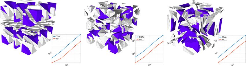
a closed geometric shape S is the locus of the points internal to S from which the
whole shape S is visible. The kernel of a convex shape coincides with the shape
itself, while the concept is particularly interesting for non-convex shapes and in
particular, polytopes. The kernel of non-convex shapes can also be empty, as in
the case of non simply-connected objects for which it is always empty.
    In the two-dimensional scenario, that is when the shape is a polygon, the
standard way of computing the kernel is by intersecting appropriate half-planes
generated from its edges. This problem has been tackled since the 70s, when [22]
presented an algorithm able to perform the kernel computation in O(e log e) op-
erations, being e the number of edges of a polygon, as the intersection of e half-
edges. After that, an optimal algorithm able to run in O(n) operations over an
n−sided polygon, has been proposed in [16]. Famous computational tools and
libraries like Boost [8], Geogram [17], CGAL [14], or Libigl [15] currently im-
plement routines to compute intersections between polygons and planes, which
can be used to estimate the kernel. In the first attempts to solve the volumetric
version of the problem, for example in [20], the natural approach has been to ex-
tend the 2D method (which we call geometric) to the 3D case from a theoretical
point of view, but it was soon dismissed as unattractive for computational rea-
sons. It was replaced by a new approach (which we call algebraic) which makes
use of linear algebra and homogeneous coordinates, and that is the state of the
art for computing 3D kernels currently implemented by libraries like CGAL.
    During years, the polygon kernel computation has become popular to address
several problems based on simple polygon analysis, such as star-components
decomposition and visibility algorithms that are of interest in robotics, surveil-
lance, geometric modeling, computer vision and, recently, in the emerging field
of additive manufacturing [11].
    Today, the geometric kernel of a polytope is a pivotal information for under-
standing the geometrical quality of an element in the context of finite elements
analysis. While in the past years finite elements methods were only designed to
work on convex elements like triangles/tetrahedra or quadrangles/hexahedra [9],
recent and more complex methods like the Mimetic Finite Difference Method
[18], the Virtual Elements Method [6], the Discontinuous Galerkin Mehod [10]
or the Hybrid High Order Method [12] are able to deal with non convex poly-
topes. This enrichment of the class of admissible elements led researchers to
further investigate the concept of the geometric quality of a polytope, and to
define quality measures and metrics for the mesh elements, whether they are
poligons [4, 27] or polyhedra [24]. In this setting, the geometric kernel is often
associated with the concepts of shape regularity and star-shapedness of an ele-
ment. For example, as analyzed in [26], most of the error estimates regarding
the Virtual Elements Method (but the same holds for other polytopal methods)
are based on the theory of polynomial approximation in Sobolev spaces, assum-
ing the star-shapedness of the elements [13, 21]. As a consequence there are a
number of sufficient geometrical assumptions on the computational domain for
the convergence of the method, which require an estimate of the kernel. When
dealing with non-trivial meshes [2, 7], such quality measures/metrics/indicators
require to compute the kernel of thousands of polytopes, each of them with a

                                        2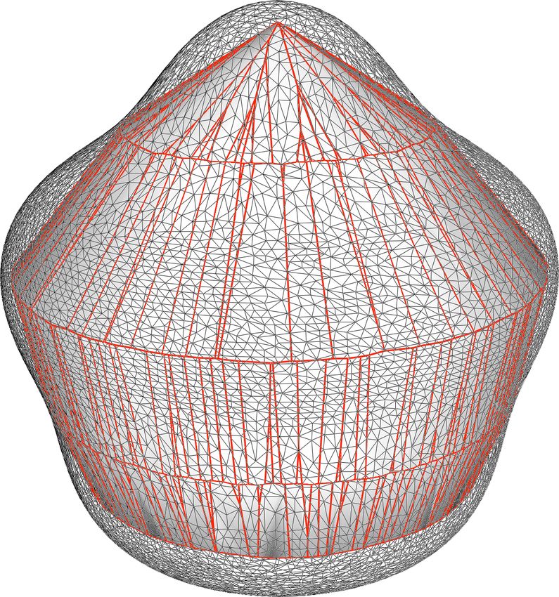
limited number of faces and vertices, in the shortest possible time.
    A preliminary algorithm for the computation of the kernel of a polyhedron
using the geometric approach was introduced in [25]. There, we experimentally
showed how this type of approach in practice can significantly outperform the
algebraic one, for instance, when polyhedral elements have a limited number of
faces and vertices or several faces are co-planar. In this paper we optimize the
algorithm, for instance preliminary estimating the position of all vertices with
respect to the planes induced by the faces, introducing the use of exact geometric
predicates [23] and a random strategy for visiting the faces of a polyhedron and
identify more rapidly polyhedra whose kernel is empty. We also simplify the
description of the algorithmic routines and we introduce new scientific results
on a larger variety of models that confirm the validity of a geometry-based kernel
algorithm.
    The paper is organized as follows. In Section 2 we introduce some notation
and discuss the difference between the geometric and the algebraic approach. In
Section 3 we detail the algorithm for the construction of the kernel of a polyhe-
dron. In Section 4 we exhibit some examples of computed kernels and analyze
the performance of the algorithm with comparisons with an implementation of
the algebraic approach and with its previous version [25]. In Section 5 we sum
up pros and cons of the algorithm and draw some conclusions.

2     Preliminary concepts
We introduce some notations and preliminary concepts that we will use in the
rest of the paper.

2.1    Notations
We define a polyhedron as a finite set of plane polygons such that every edge
of a polygon is shared by exactly one other polygon and no subset of polygons
has the same property [20]. The vertices and the edges of the polygons are
the vertices and the edges of the polyhedron; the polygons are the faces of the
polyhedron. In this work we only consider simple polyhedra, which means that
there is no pair of nonadjacent faces sharing a point.
     A polyhedron P is said to be convex if, given any two points p1 and p2 in
P , the line segment connecting p1 and p2 is entirely contained in P . It can be
shown that the intersection of convex polyhedra is a convex polyhedron [20].
Two points p1 and p2 in P are said to be visible from each other if the segment
(p1 , p2 ) does not intersect the boundary of P . The kernel of P is the set of points
in the interior of P from which all the points in P are visible. The first obvious
consideration is that the kernel of a polyhedron is a convex polyhedron. If P
is convex its kernel coincides with its interior, because any two points inside a
convex polyhedron are visible from each other. A polyhedron may also not have
a kernel at all; in this case we say that its kernel is empty. Last, a polyhedron
P is called star-shaped if there exists a sphere, with non-zero radius, completely

                                          3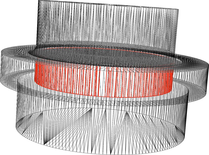
contained in its kernel. A polyhedron is star-shaped if and only if its kernel
is not empty, therefore star-shapedness can be thought as an indicator of the
existence of a kernel. Star-shapedness is weaker than convexity, and it is often
used in the literature as many theoretical results in the theory of polynomial
approximation in Sobolev spaces rely on this condition [13, 21].

Figure 2: A sequence of parametric polyhedra whose kernel is progressively
shrinking. The kernel is the polyhedron delimited by the red edges.

    In order to give a visual example of these concepts, in Fig. 2 we present a
parametric object shaped like a tent, with the parameter regulating the height
of the “entrance” from the basis. This object is not convex, but in the first
examples it is star-shaped and it has a proper kernel, delimited by the red
edges. As the parameter increases, the set of points from which the whole
polyhedron is visible becomes smaller, and so does the star-shapedness radius.
The last example of Fig. 2 is not star-shaped anymore, i.e. the kernel is empty.

2.2    The algebraic approach to the kernel computation
As observed in Section 1, the state of the art algorithm for the computation
of the kernel of a polygon follows a geometric approach: the kernel is found as
the intersection of half-planes originating from its edges. We use the term “ge-
ometrical” because the algorithm computes repeatedly a sequence of geometric
intersections between polygons and planes. This idea was afterwards optimized
until obtaining an algorithm able to run in O(n) operations, which has been
proven to be optimal [16].
    When facing the 3D version of the problem, one natural way could be to
extend the 2D algorithm, which is well studied and documented, to the higher
dimension. The problem with the 3D case is that, whereas two convex polygons
with respectively n1 and n2 vertices can be intersected in time O(n), being
n = n1 + n2 , two convex polyhedra with the same parameters are intersected in
time O(n log n), thus the generalization of the two-dimensional instance would
yield an O(n log2 n) algorithm. This is in contrast with the result shown in [20],
where a lower bound for the intersection of convex polyhedra is established
at O(n log n). Therefore the geometric approach to the 3D problem was soon
dismissed as unattractive, and alternative ways have been explored.
    A new algorithm was formulated, based on the so-called “double duality
trick”, which makes use of linear algebra and homogeneous coordinates. Thanks
to this algebraic approach, described in [20, Section 7.3.2], it is possible to

                                        4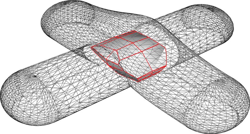
compute the intersection of n half-spaces in time O(n log n) [20]. This algorithm
can be implemented inside the framework of the CGAL library, although there
is currently not an explicit routine for computing the kernel of a polyhedron
and one has to connect the function for the intersection of half-spaces to the
polyhedron data structure. The whole routine implies:

  1. solving a linear problem to find a point in the interior of the polyhedron;
  2. translating the polyhedron so that the interior point is the origin;
  3. calculating the dual polyhedron, defined as the convex hull of the vertices
     dual to the original faces in regard to the unit sphere (i.e., halfspaces at
     distance d from the origin are dual to vertices at distance 1/d);
  4. calculating the resulting polyhedron, which is the dual of the dual poly-
     hedron;
  5. translating the origin back to the interior point.

    While from a theoretical point of view the cited results are indubitable, we
believe that in many practical situations the geometric approach could perform
better than the algebraic one. This is due to the fact that the cost of solving
a linear problem cannot fall below a certain bound, while the intersection of
half-spaces can become extremely cheap in some circumstances. For instance if
the number of faces and vertices of the polyhedron is low, this method could be
more efficient than the algebraic one, and there may be other situations in which
one could take advantage of a wise treatment of the geometrical operations.

2.3    Data structure
We adopt the following data structure inherited by the cinolib library [19], in
which the code has been written:
   • Points: array of unordered 3D points.
   • Face: array of unsigned integers associated to a Points array, representing
     the indices of the vertices of a face ordered counter-clockwise.

   • Polyhedron: struct composed by a field verts of type Points containing
     the vertices and a field faces of type array  containing the faces
     of a polyhedron.
   • Plane: class defining a plane in the Hessian form, composed by a 3D point
     n indicating the unit normal of the plane (i.e. the a, b, c coefficients of the
     plane equation) and a number d indicating the distance of the plane from
     the origin (i.e. the d coefficient of the plane equation). The plane class
     also contains three additional points p1 , p2 , p3 lying on the plane, useful
     for the Shewchuck exact predicates [23].

                                         5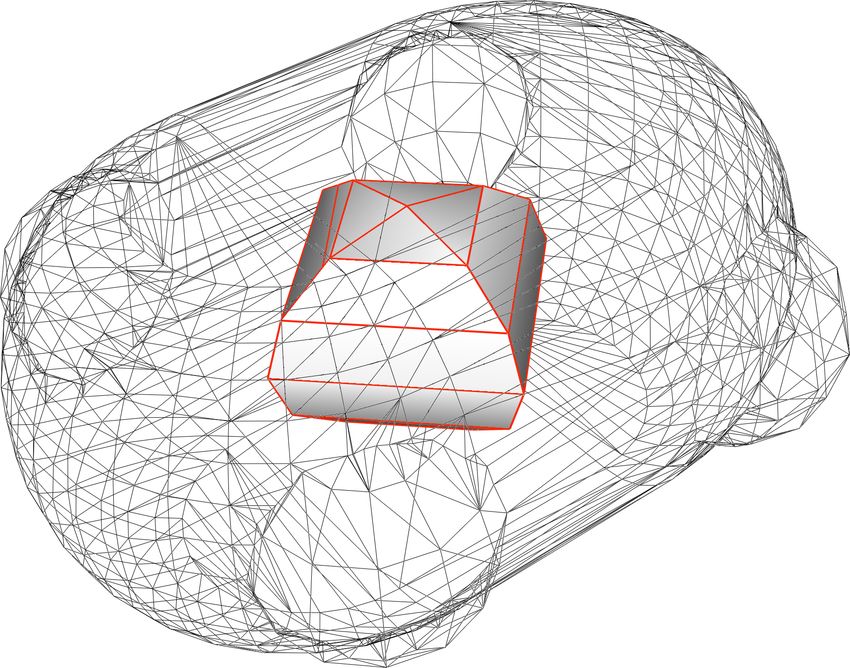
• Sign: array of labels (BELOW, ABOVE or INTER) used to store infor-
      mation on the position of the elements of a polyhedron (points, edges or
      faces) with respect to an unspecified plane.
Given a plane p, the elements of a polyhedron are classified as follows:

    • A point v is labelled as BELOW, ABOVE or INTER provided that the
      function orient3d (p.p1 , p.p2 , p.p3 , v) in the Shewchuck exact predicate li-
      brary [23] is negative, positive or zero, within a tolerance of 10−8 ;
    • An edge e is labelled as BELOW (resp. ABOVE) if both its endpoints
      are BELOW or INTER (resp. ABOVE or INTER), and as INTER if one
      point is ABOVE and the other one is BELOW.
    • A face f is labelled as BELOW if all of its points are BELOW, as ABOVE
      if none of its points is BELOW and as INTER otherwise.
The classification of points is computed at the top level of the algorithm with
Shewchuck exact predicates, defining the symbol CINOLIB USES EXACT PREDICATES
at compilation time. For edges and faces instead, we define a function classify(S)
which determines the classification of and edge or a face from an array S of type
Sign containing the classification of its points. The introduction of the labels
and the points evaluation at the beginning of the process are two main compu-
tational novelties with respect to the previous version of the algorithm [25].

3     Polyhedron kernel algorithm
In this section, we illustrate our method for computing the kernel of a polyhe-
dron with a geometric approach. It has a modular structure composed of four
nested algorithms, each one calling the next one in its core part. It is modular
in the sense that each algorithm can be entirely replaced by another one per-
forming the same operation(s). This property is particularly useful for making
comparisons: one could, for instance, use different strategies for computing the
intersection between a polygon and a plane and simply replace Algorithm 3,
measuring the efficiency from time to time.

3.1    Polyhedron Kernel
With Algorithm 1 we tackle the general problem: given a polyhedron P , we
want to find the polyhedron K representing its kernel. In addition to P we also
need as input an array containing the outwards normals of its faces, as it is not
always possible to determine the orientation of a face only from its vertices (for
example with non-convex faces). We require the face normals explicitly, and
not simply a boolean indicating the faces orientation, because these points will
be used to define the planes containing the faces of P .
   We initialize K with the axis aligned bounding box (AABB) of P , i.e. the
box with the smallest volume within which all the vertices of P lie, aligned with

                                          6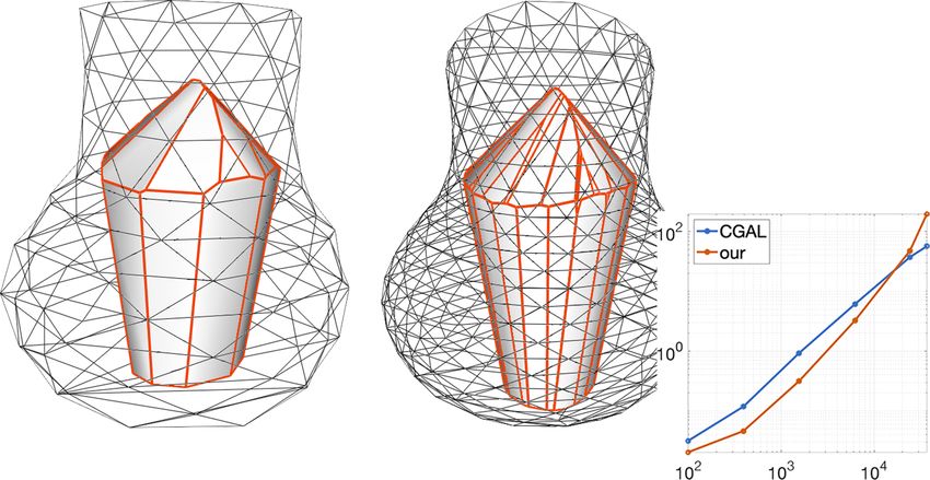
the axes of the coordinate system. Then we recursively “slice” K with a number
of planes, generating a sequence of convex polyhedra Ki , i = 1, . . . , #P.faces,
such that Ki ⊆ Ki−1 . For each face f of P we define the plane p containing
its vertices and with normal vector given by the opposite of the face normal
N (f ), that is to say, p.n := −N (f ). We consider the plane together with the
direction indicated by p.n, which is equivalent to considering the half-space
originating in p and containing its normal vector. Given this plane, in a Sign
array S we store the classification of all the points in K.verts according to
their position with respect to p. For improving the efficiency, we can set the
sign of all points belonging to f to zero without evaluating their position. In
general p will separate K into two polyhedra, and between those two we keep
the one containing the vector p.n, which therefore points towards the interior of
the element. This operation is performed by the Polyhedron-Plane Intersection
algorithm detailed in Section 3.3, which replaces K with the new polyhedron.
     The order in which we consider the faces is not relevant from a theoretical
point of view, but turns out to have a huge impact on the performance. For
instance, if we imagine to compute the kernel of a “ring”, which is obviously
empty, visiting the faces in the order they are stored may take a very long time,
especially if the tessellation of the object is fine. This is because, generally,
the faces of a tessellated model are numbered somehow coherently with their
neighbors. For this reason, we optionally propose to visit the faces in random
order, or shuffle P.f aces, and to return an empty polyhedron if after a “slice” K
has less than three faces. In this way, the empty kernel of a ring with thousands
of faces could be detected in just three or four iterations. When this command
is turned on, we say the algorithm is run in shuffle mode.
     We point out that cutting a convex polyhedron with a plane will always
generate two convex polyhedra, and since we start from the bounding box (which
is convex), we are guaranteed that K will always be a convex polyhedron. No
matter how weird the initial element P is, from this point on we will only be
dealing with convex polyhedra and convex faces. Last, we could as well start
with considering the polyhedron’s convex hull instead, but it would be less
efficient because the convex hull costs in general O(n log n) while the AABB is
only O(n), and we would still need to intersect the polyhedron with each of its
faces.

3.2    Polyhedron-Plane Intersection
With the second algorithm we want to intersect a polyhedron P with a plane p,
given in S the position of the vertices of P with respect to p. The intersection will
in general determine two polyhedra, and between these two we are interested in
the one containing the normal vector of p (conventionally called the one “above”
the plane and indicated with A). This algorithm is inspired from [1], where the
authors define an algorithm for the intersection of a convex polyhedron with an
half-space.
    The first part of Algorithm 2 is called the “clipping” part (recalling the
terminology from [1]) and consists in clipping each face of P with the plane

                                         7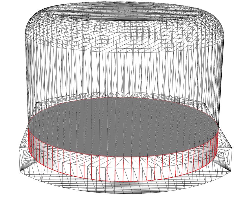
Algorithm 1 Polyhedron Kernel
Input: Polyhedron P , Points N (faces normals);
Output: Polyhedron K
 1: K := AABB of P ;
 2: [optional] shuffle P.f aces;
 3: for Face f in P.f aces do
 4:     Plane p := plane containing f with normal −N (f );
 5:     Sign S := orient3d(p.p1 , p.p2 , p.p3 , K.verts);
 6:     K := Polyhedron-Plane Intersection(K, S, p);
 7:     if size(K.f aces) < 3 then return NULL;
 8:     end if
 9: end for
10: return K;

                  (a)                                     (b)

Figure 3: Intersection of a polyhedron with a plane: (a) clipping and (b) capping
of a cube.

                                       8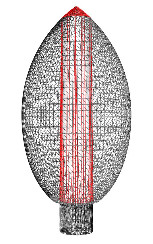
p, see Fig. 3(a). It corresponds to the for loop: we iterate on P.faces, each
time extracting from S the labels fs of the vertices fv of the current face and
using the classify function. Faces classified as BELOW are discarded, ABOVE
faces are added to A together with their vertices, and INTER faces are split by
the Polygon-Plane Intersection algorithm. While we visit every face only once,
the same does not hold for vertices, therefore we check if a vertex is already in
A.verts before adding it.
    This simple idea of checking in advance the faces classification resolves sev-
eral implementation issues and in some cases significantly improves the efficiency
of the algorithm. By doing this, we make sure that only the faces properly in-
tersected by the plane are passed to Algorithm 3, so that we do not need to
implement all the particular cases of intersections in a single point or along an
edge or of faces contained in the plane. In addition, for every face not passed
to Algorithm 3 we have an efficiency improvement, and this happens frequently
in models with many coplanar faces like the ones considered in Section 4.2.
    If, at the end of this step, A contains at least three INTER points, given
that A and all its faces are convex, these vertices will define a “cap” face of
A completely contained in p, see Fig. 3(b). We can optimize the algorithm by
storing in a Sign array the classification of the vertices in A, updating it with
the sign of every vertex added in the switch loop. Note that in this case we do
not need to use orient3d : we already know the sign of the old vertices and the
new vertices will obviously be of type INTER. In our data structure, the vertices
of the faces are ordered counter-clockwise (CCW): in order to sort the points
contained in capV we project them onto a plane, drop one coordinate and apply
the algorithm proposed in [5] for 2D points. Note that if the cap face was not
convex it would make no sense to order its vertices, but the intersection between
a plane and a convex polyhedron will always generate convex faces. Last, we
need to check that this new face is not already present in A: for example if p
was tangent to P along a face, this face could be added to A both as an ABOVE
face and as a cap face. If this is not the case, we add capF to A.f aces but we
do not need to add any vertex from capV, as we can assume they are all already
present in A.verts.

3.3    Polygon-Plane Intersection
Algorithm 3 describes the intersection of a polygon (representing a face of the
polyhedron), defined by an array of 3D points polyV and an array of indices
polyF, with a plane p. As before, we also require as input an array polyS con-
taining the position of the vertices of polyV with respect to p. In analogy to
Algorithm 2, the intersection will in general determine two polygons and we
are only interested in the one above the plane, see Fig. 4(a), defined by points
aboveV and indexes aboveF. We generically say that a vertex v is added to above
meaning that v is added to aboveV and its index idv is added to aboveF.
    This time we iterate on the edges of polyF, extract the signs s1 , s2 of the
edge endpoints and switch between the three possible classifications of the edge.
In order to avoid duplicates, for each couple of consecutive points v1 , v2 , we

                                        9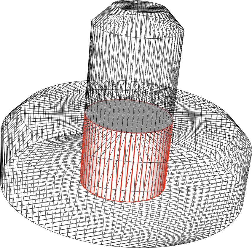
Algorithm 2 Polyhedron-Plane Intersection
Input: Polyhedron P , Sign S, Plane p
Output: Polyhedron A
 1: for Face f in P.f aces do
 2:     Points fv := vertices in P.verts relative to f ;
 3:     Sign fs := S|fv
 4:     switch classify(fs ) do
 5:         case BELOW break;
 6:         case ABOVE
 7:             A.verts ← fv , A.f aces ← f ;
 8:         case INTER
 9:             (V,F ):=Polygon-Plane Intersection(fv , f, fs , p);
10:             A.verts ← V, A.f aces ← F ;
11: end for
12: Points capV := vertices in A.verts which are INTER;
13: if size(capV ) < 3 then return A;
14: end if
15: Face capF := indices of capV vertices ordered CCW;
16: if capF ∈ / A.f aces then A.f aces ← capF ;
17: end if
18: return A;

only accept to add to above the second point v2 or the intersection point v, but
never v1 . We are here taking advantage of the fact that all faces are oriented
coherently.
     If the edge is of type BELOW we ignore it unless v2 is INTER (i.e. it lies
exactly on the plane), in which case we add it to above. In case of ABOVE
edges we add v2 to above. For edges of type INTER we perform the Line-Plane
Intersection algorithm and find a new point v. Its index idv will be equal to
the maximum value in polyF plus one, just to make sure that we are not using
the index of an existing point. We always add v to above, and if v1 is BELOW
we also add v2 . As already noted in Section 3.2, treating separately the weak
intersections (the BELOW and ABOVE cases) makes the code simpler and more
efficient.

3.4    Line-Plane Intersection
This last algorithm computes the intersection point between a line, given as a
couple of vertices, and a plane. It is a very simple and well known procedure,
and we report it here only for completeness.
   The intersection vertex v is defined as the linear combination of vertices v1
and v2 , with a coefficient t which may also fall outside the standard range [0, 1].
The coefficient t is found as the negative ratio between two scalar products
involving the plane normal n and a generic other point on the plane s, other

                                         10
(a) (b)
Figure 4: (a) Intersection between a polygon and a plane, with the above part
coloured in green. (b) Intersection between a line and a plane.
Algorithm 3 Polygon-Plane Intersection
Input: Points polyV, Face polyF, Sign polyS, Plane p.
Output: Points aboveV, Face aboveF.
1: for i = 1 : size(polyF ) do
2: id1 := polyF (i), id2 := polyF (i + 1);
3: v1 := polyV (id1 ), v2 := polyV (id2 );
4: s1 := polyS (id1 ), s2 := polyS (id2 );
5: switch classify(s1 , s2 ) do
6: case BELOW
7: if v2 is INTER then
8: aboveV ← v2 , aboveF ← id2 ;
9: end if
10: case ABOVE
11: aboveV ← v2 , aboveF ← id2 ;
12: case INTER
13: v := Line-Plane Intersection(v1 , v2 , p);
14: idv := max(polyF )+1;
15: aboveV ← v, aboveF ← idv ;
16: if v1 is BELOW then
17: aboveV ← v2 , aboveF ← id2 ;
18: end if
19: end for
20: return aboveV, aboveF ;
11than v1 and v2 see Fig 4(b). The normal is p.n, and for the point s we can
use one of the three points on the plane p.p1 , p.p2 , p.p3 . If the denominator D
vanishes, it means either that the line is contained in the plane (if N = 0 as
well) or that the line does not intersect the plane. We treat these exceptions
as errors because in Algorithm 3 we only call this algorithm after checking that
the edge (v1 , v2 ) properly intersects the plane p.
Algorithm 4 Line-Plane Intersection
Input: vertices v1 , v2 , Plane p.
Output: vertex v.
1: N := (p.n) · (v1 − p.p1 );
2: D := (p.n) · (v2 − v1 );
3: assert(D! = 0)
4: t := −N/D;
5: return v := v1 + t (v2 − v1 );
3.5 Computational complexity
Making advantage of the modular organisation of our algorithms, we can es-
timate separately the computational cost of each algorithm and then include
them into a single formula.
Let us consider the case of an input polyhedron P with nv vertices and nf
faces. In Algorithm 1 we start by computing the polyhedron’s AABB, which
is O(nv ), then for each face we estimate the position of the vertices of K with
respect to a plane with orient3d. Unfortunately, we have to re-compute the signs
of all the nkv vertices of K at every iteration, as from one step to the other the
plane changes: this means O(nkv nf ) operations. At step zero we have nkv = 8,
being K the bounding box; then in the worst case, that is if the object is convex,
it can grow up to nv because K coincides with P . If the object is not convex,
nkv can remain significantly lower than nv , which translates in a much lower
computational cost. In both cases, the difference between nkv and nv is also
related to the number of coplanar faces of the model, which get agglomerated
into a single face in the kernel with a consequent reduction of the number of
vertices. If the kernel is empty, whenever we end up with less than three faces
the algorithm stops, therefore we can replace nf with the number of iterations
needed to detect the non star-shapedness. This number cannot be estimated
precisely, but we can drastically reduce it with the shuffle mode.
The good news is that once that we have the sign of all the vertices with
respect to all the planes we are essentially done: the computational costs of
Algorithms 2 and 3 is all about visiting arrays and copying parts of them into
other arrays, and Algorithm 4 only consists of 4 operations. We point out that
navigating and duplicating arrays has a negligible cost in this scenario as the
faces of a generic polyhedron hardly contain more than 10 vertices. The only
relevant operation in Algorithm 2 is the sorting of the vertices of the cap face,
12which does not always exist. This is done with a QuickSort routine which is on
average O(n log n) for a cap face with n vertices. Since n is much smaller than
nkv and the number of cap faces is always smaller than nf , this cost is negligible
compared to O(nkv nf ).
In summary, we can set an upper bound to the computational cost of our
algorithm at O(nv nf ), but both nv and nf can significantly decrease if the model
is not convex or has coplanar faces, and even more if it is not star-shaped. In
the next section we will show how in practice, on small polyhedra or on objects
with many co-planar faces, the geometric method works in a computational
time which is smaller than the one of the algebraic approach, and it is still
competitive on many examples, even complex ones.
4 Tests and discussions
We test our method in different settings, comparing its performance to the
results obtained using our implementation of the algebraic method in CGAL.
The comparison of the current method, including the shuffle version, and its
previous version in [25] is presented in Section 4.4.
Experiments have been performed on a MacBook Pro equipped with a 2,3
GHz Intel Core i5 processor with four CPUs and 16GB of RAM. Source code is
written in C++ and it is accessible at https://github.com/TommasoSorgente/
polyhedron_kernel, together with all datasets.
In the following subsections we will present some plots and tables: we point
out here some remarks on the notation adopted. Regarding plots, we colour
the CGAL computational time in blue and our computational time in red, both
in logarithmic scale. On the x−axis, depending from the context, we have
the number of elements in the mesh or the number of vertices of the single
model. In the several tables presented we first report the number of elements or
vertices of the mesh. Since all the considered objects have genus zero and their
surface is purely triangular, Euler’s formula states that the number of faces is
approximately equal to twice the number of vertices. Therefore we only indicate
the number of vertices, but the number of faces is easily computable. Then the
computational times (in seconds) are shown, and the ratio between CGAL time
and ours. Note that ratios are computed from the original time values while in
the tables we indicate truncated times, therefore they do not exactly correspond
to the division between the values in the previous columns.
4.1 Polyhedral meshes
First, we test our algorithm in the setting it was developed for, i.e. the computa-
tion of the kernels of elements in a 3D tessellation. To do so, we used the datasets
from [24], available for download at https://github.com/TommasoSorgente/
vem-indicator-3D-dataset. The meshes contained in these datasets are typ-
ical examples of tessellations which can be found in numerical analysis for the
approximation of a PDE. We focus our attention on the polyhedral datasets:
13Figure 5: Polyhedral meshes and time plots from datasets poly-parallel, poly-
poisson and poly-random, with non-tetrahedral elements highlighted in blue.
poly-parallel, poly-poisson and poly-random. Each of them contains five tessel-
lations of the unit cube with decreasing mesh size, from 100 to 100K vertices.
The resulting meshes contain between 100 and 600K elements, most of which are
tetrahedra but 20% of them are generic polyhedra (in blue in Fig. 5), obtained
by the union of two tetrahedra.
Figure 6: Examples of non-convex elements found in polyhedral meshes from
Section 4.1 and relative kernels.
Non-tetrahedral elements are generated by the agglomeration of two tetra-
hedral elements, therefore they may also be non convex, see Fig. 6.
In Table 1 we report, for each mesh of each dataset, the number of elements,
the computational times for both methods and the ratio between the CGAL time
and ours. Moreover, at the bottom of Fig. 5 we plot the times against the number
of elements in the mesh. It is visible how both methods scale linearly with
respect to the number of elements, since the kernel of the elements is computed
separately and independently for each element. Our method performs 8 to 11
times faster than CGAL, which approximately means one order of magnitude.
As the elements of these meshes have either 4 faces if they are tetrahedra or
6 faces if they are the union of two tetrahedra, computing their kernel in a
geometrical way results much faster than solving a linear problem. In this case
we did not use the shuffle mode, as the number of faces was so small that the
visiting order resulted not relevant.
14Table 1: Computational times for polyhedral meshes.
dataset #elements our CGAL ratio
poly-parallel 130 0.04 0.21 4.89
1647 0.17 1.79 10.69
16200 1.68 19.4 11.55
129600 13.94 142.36 10.21
530842 53.47 588.43 11
poly-poisson 140 0.04 0.3 8.05
1876 0.29 2.54 8.91
16188 2.64 24.79 9.38
146283 24.24 212.23 8.75
601393 86.77 770.66 8.88
poly-random 147 0.03 0.19 6.8
1883 0.28 2.62 9.41
18289 2.91 27.11 9.33
161512 26.51 228.08 8.6
598699 80.15 735.55 9.18
4.2 Refinements
As a second setting for our tests, instead of increasing the number of elements we
wanted to measure the asymptotic behaviour of the methods as the number of
faces and vertices of a single element explodes. We selected two polyhedra from
the dataset Thingi10K [28]: the so-called spiral (ThingiID: 60246) and vase
(ThingiID: 85580). These models are given in the form of a surface triangular
mesh but we treat them as single volumetric cell, analyzing the performance
of both algorithms as we refine them. In Table 2 we report the computational
times and the ratio for each refinement.
The spiral model is refined through a midpoint strategy: each face is subdi-
vided by connecting its barycenter to its other vertices. As a consequence, the
planes induced by its faces remain the same and the kernels of the refined mod-
els are all equal (Fig. 7). On this example our method performs on average 5.77
times better that the algebraic method (see Table 2), and the computational
time scales with a constant rate (see the plot in Fig. 7). Our implementation
takes advantage of the fact that Algorithm 2 recognises the several coplanar faces
and always performs Algorithm 3 the same number of times, independently of
the number of faces.
The vase model is more complex, as it presents a curved surface which
generates a lot of different planes defining the kernel. Moreover, we refined this
model using the Loop’s algorithm and this generated faces lying on completely
new planes. This explains the difference between the two kernels in Fig. 8: the
general shape is similar but the more faces we add to our model the more faces we
find on the resulting kernel. Our geometric method improves the performance
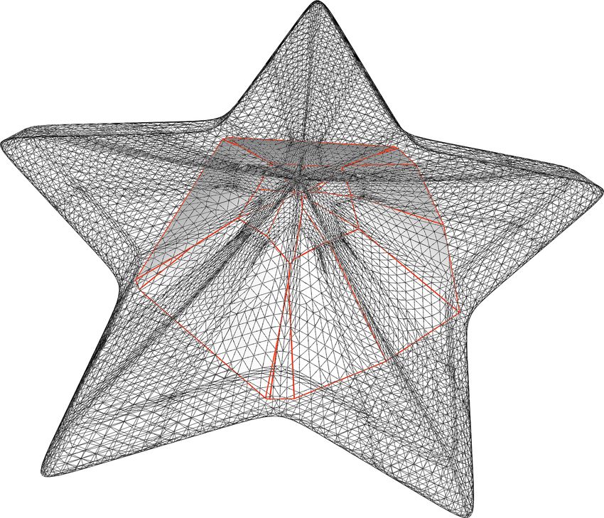
15Figure 7: Original spiral model and its first refinement, with identical kernels.
of the algebraic one by a factor around 2 in the first refinements, but in the last
two meshes the complexity increases drastically and CGAL results faster (see
Table. 2). In this case, an efficient treatment of the faces is not sufficient to hide
the quadratic nature of the geometric approach. Even the shuffle mode did not
particularly improve the performance, being the object star-shaped.
4.3 Complex models
Last, we try to compute the kernel of some more complex models, taken again
from the dataset Thingi10K and treated as single volumetric cells. Even if our
method is designed for dealing with polyhedra of relatively small size, as we
already saw in Section 4.2 our algorithms are still able to compute the kernel of
objects with thousands of vertices and faces. We filtered the Thingi10K dataset
selecting only “meaningful” models: objects with one connected component,
genus zero, Euler characteristic greater than zero, closed, not degenerate and
of size smaller than 1MB. Note that, even applying these filters, the majority
of the models are not star-shaped, i.e. with empty kernel. We discarded a few
models for computational and stability reasons, for instance because one of the
two algorithms failed to process them. The final collection, which we will call
the Thingi dataset, contains exactly 1806 distinct volumetric models.
In Fig. 9 we show the times distribution for the whole Thingi dataset, with a
particular focus on the difference between models with empty kernel and mod-
els with non-empty kernel. Globally, the overall cost of computing all kernels is
16Figure 8: Original vase model and its first refinement: small perturbations in
the faces lead to slightly different kernels.
Table 2: Computational times for the spiral and vase refinements.
mesh #vertices our CGAL ratio
spiral 64 0.004 0.01 3.07
250 0.007 0.04 6.27
994 0.02 0.14 6.56
3970 0.08 0.43 5.38
15874 0.32 1.77 5.54
63490 1.05 8.24 7.86
vase 99 0.02 0.03 1.55
390 0.04 0.12 2.56
1554 0.31 0.92 2.94
6210 3.24 6.1 1.88
24261 47.49 37.24 0.78
36988 196.7 56.75 0.29
17Figure 9: Thingi dataset times. From left to right: all Thingi dataset, models
with empty kernel, models with non-empty kernel.
173 seconds with our method against 518 seconds with CGAL, for an improve-
ment of 3 times. When the kernel is empty our algorithm is always faster than
CGAL: the main reason for this is the usage of the shuffle mode, which makes
it extremely cheap to recognise non star-shaped elements. When the model is
star-shaped the distinction between the two methods is not so clear anymore,
as the results mainly depend on the shape and size of the object.
To further investigate on this point, in Fig. 10 we present the kernel com-
putation of 10 selected star-shaped examples from this dataset. In the top
row we have models on which the geometric method is by far more efficient:
plus (ThingiID: 1120761), star (ThingiID: 313883), flex (ThingiID: 827640) and
cross (ThingiID: 313882). In the middle row, models for which the performance
are similar: part (ThingiID: 472063), super-ellipse (ThingiID: 40172), bot-eye
(ThingiID: 37276) and button (ThingiID: 1329185). Then in the bottom row we
show models on which the algebraic method is preferable: rt4-arm (ThingiID:
39353), ball (ThingiID: 58238), acorn (ThingiID: 815480), muffin (ThingiID:
101636). The computational times, together with the ones relative to the whole
dataset, are reported in Table 3.
Once again, we notice that the size of the model impacts on the performance
of our method. Looking at Fig. 9 we can see how the models for which our
method performs worse than CGAL are all in the right part of the plane, relative
to models with a high number of vertices. At the same time, the number of
vertices of the element, by itself, is not sufficient to justify the supremacy of one
method over the other. For example, models star and flex have very different
sizes and times, but their ratio is quite similar; the same holds for models parts
and super-ellipse or ball and acorn.
The shape of the object also plays an important role: over models with
numerous adjacent co-planar faces like plus, star (whose bottom is completely
flat) and cross our method is preferable even when the size grows. As already
seen in Section 4.2, the presence of coplanar faces significantly improves the per-
formance of our method. Vice-versa, over elements with significant curvatures
like rt4-arm, acorn or muffin, the algebraic method performs similarly or better
than ours even on relatively small models like bot-eye. Over these models it is
still possible to compute a correct kernel with the geometric approach, but the
18plus star flex cross
part super-ellipse bot-eye button
rt4-arm ball acorn muffin
Figure 10: Examples of our kernel evaluation for complex models. In the top
row models on which the geometric method is more efficient, in the middle
models for which the performance are similar and in the bottom row models on
which the algebraic method is preferable.
ratio between CGAL time and ours is in the order of 10−1 or even 10−2 .
4.4 Comparison with the previous version
With respect to its introduction in [25], we believe that the algorithm is now
more easy to read and to understand, thanks to the introduction of labels for
storing the position of vertices, edges and faces with respect to a plane. Another
significant difference is that the evaluation of the position of the vertices is
now computed once and for all, at the top level (in Algorithm 1), while in
the previous version every algorithm contained some vertices evaluations: this
further reduced the computational complexity. In addition, we switched from
the inexact predicates (in [25] we used the equivalent of orient3d-fast) to the
exact orient3d, which resulted in an increasing precision in the treatment of
nearly-coplanar faces, for a small extra cost which was easily compensated by
the other improvements. This switch required a small modification of the Plane
19Table 3: Computational times for complex models. The first number relative to
Thingi dataset indicates the number of models instead of the number of vertices.
mesh #vertices our-shuffle CGAL ratio
plus 448 0.004 0.09 22.75
star 9633 0.4 5.15 12.93
flex 834 0.02 0.27 12.76
cross 3914 0.19 2.1 11.12
part 5382 2.58 6.94 2.69
super-ellipse 290 0.02 0.04 2.05
bot-eye 453 0.03 0.03 0.96
button 1227 0.1 0.08 0.75
rt4-arm 655 0.13 0.09 0.67
ball 660 0.24 0.04 0.15
acorn 4114 4.35 0.55 0.13
muffin 8972 11.73 0.54 0.04
Thingi dataset 1806 172.88 518.2 2.99
class: in view of the usage of orient3d, for every plane we also store three points
on it. Last, the introduction of the shuffle mode made the computation of the
kernels of non star-shaped objects almost immediate, marking a huge difference
with respect to the algebraic method and our previous implementation. In
Table 4 we report the differences between the old version of the algorithm and
the current version in standard and in shuffle mode. Over the meshes from
Section 4.1 there is almost no differences between the three versions. For refined
models, there is an improvement of a factor 2 in the computation of the vase
refinement (we report the sum of the times for all the refinements). With
complex models we have the greatest differences; in these cases we can also
appreciate the advantage brought by the shuffle mode, which was not significant
in the other tests.
5 Conclusions
We presented an algorithm for the computation of the kernel of a polyhedron
based on the extension to the 3D case of the geometric approach commonly
adopted in two dimensions. With respect to [25] we have optimized the algo-
rithm in several ways: we now perform all the vertices comparisons in a single,
preliminary step; we have introduced the use of exact geometric predicates and
a random visiting strategy of the faces that considerably improve the perfor-
mance of the method over non star-shaped, complex objects. The algorithm
showed up to be robust and reliable, as it computed successfully the kernel of
every considered polyhedron. The efficiency of our algorithm is compared to the
CGAL implementation of the algebraic approach to the problem. From a the-
oretical point of view, the computational complexity evaluation of Section 3.5
20Table 4: Performance comparison between the current implementation and the
one presented in [25]. Only models with significant differences are reported.
mesh our-shuffle our our [25]
spiral (sum) 1.04 1.01 1.03
vase (sum) 245.61 194.91 495.63
cross 0.19 4.15 9.14
part 2.58 5.22 12.7
bot-eye 0.03 0.17 0.25
rt4-arm 0.13 0.14 0.21
button 0.1 0.11 0.15
ball 0.24 0.28 0.58
acorn 4.35 276.13 626.72
muffin 11.73 58.62 129.38
suggests that our method is in general quadratic, while the algebraic approach
has a lower bound at n log(n). Nonetheless, we proved all across Section 4 that
in several circumstances our approach outperforms the algebraic one.
The geometric approach showed up to be significantly faster than the al-
gebraic one when dealing with models satisfying at least one of the following
conditions:
1. the size of the model is small;
2. the model contains a significant number of co-planar faces;
3. the kernel is empty.
Our method performs significantly better than the algebraic approach over poly-
hedra with a limited number of vertices and faces, as shown in Section 4.1,
making it particularly suitable for the analysis of volumetric tessellations with
non-convex elements. Indeed, we point out that our algorithm is specifically de-
signed to be used with simple polyhedra, possibly composing a bigger and more
complex 3D model, rather than with a complete model itself. This behaviour is
particularly evident with model vase from Section 4.2. As long as the size of the
model remains reasonable our method is faster than CGAL, then over a certain
bound the algebraic method becomes more efficient. Again, models like super-
ellipse or flex from Section 4.3 have few or zero co-planar faces and a significant
kernel, but the size of these meshes is small and the geometric approach offers
better performance. According to Fig. 9, a bound on the number of vertices
could be possibly set at around 103 . When the size of the polyhedron increases,
our method is still particularly efficient if the model has numerous co-planar
faces, due for instance to the presence of flat regions on the surface. This is a
very common situation in models representing mechanical parts. For instance,
models star and part from Section 4.3 present large flat regions despite having a
21significant size, and again the geometric approach is faster on these models. An-
other scenario in which the geometric approach overperforms the algebraic one
is with non star-shaped objects. The differences in this case are so evident that
one could even imagine to use our algorithm to understand, in few iterations in
shuffle mode, if a model is actually star-shaped or not, even without computing
the proper kernel. On the other side, the algebraic approach is likely to re-
main preferable over domains which do not satisfy any of the above conditions:
star-shaped objects with thousands of vertices and high surface curvature.
In conclusion, with this work we do not aim at completely replacing the al-
gebraic approach for the kernel computation but instead to give an alternative
which can be preferred for specific cases, such as the quality analysis of the
elements in a 3D tessellation, in the same way as bubble-sort is to be preferred
to optimal sorting algorithms when dealing with very small arrays. As a fu-
ture development, we plan to integrate in our algorithm the promising indirect
predicates introduced in [3]. Numerical problems remain a critical issue in the
computation of geometric constructions like the kernel, independently of the
approach adopted. We believe indirect predicates could enormously help in en-
hancing the robustness of the algorithm. Moreover, we plan to include this tool
in a suite for the generation and analysis of tessellations of three dimensional
domains, aimed at PDE simulations. The kernel of a polyhedron has a great
impact on its geometrical quality, and the geometrical quality of the elements
of a mesh determines the accuracy and the efficiency of a numerical method
over it. We are therefore already using this algorithm in works like [27] for bet-
ter understanding the correlations between the shape of the elements and the
performance of the numerical simulations, and be able to adaptively generate,
refine or fix a tessellation accordingly to them.
Acknowledgements
We would like to thank Dr. M. Manzini for the precious discussions and sug-
gestions, and all the people from IMATI institute involved in the CHANGE
project. Special thanks are also given to the anonymous reviewers for their
comments and suggestions.
This work has been partially supported by the ERC Advanced Grant CHANGE
contract N.694515.
References
[1] Hyung T. Ahn and Mikhail Shashkov. Geometric algorithms for 3D in-
terface reconstruction. In Proceedings of the 16th international meshing
roundtable, pages 405–422. Springer, 2008.
[2] Paola F Antonietti, Michele Botti, Ilario Mazzieri, and Simone Nati Poltri.
A high-order discontinuous galerkin method for the poro-elasto-acoustic
22problem on polygonal and polyhedral grids. SIAM Journal on Scientific
Computing, 44(1):B1–B28, 2022.
[3] Marco Attene. Indirect predicates for geometric constructions. Computer-
Aided Design, 126:102856, 2020.
[4] Marco Attene, Silvia Biasotti, Silvia Bertoluzza, Daniela Cabiddu, Marco
Livesu, Giuseppe Patané, Micol Pennacchio, Daniele Prada, and Michela
Spagnuolo. Benchmarking the geometrical robustness of a virtual element
Poisson solver. Mathematics and Computers in Simulation, 190:1392–1414,
2021.
[5] Baeldung. Baeldung guides and courses. https://www.baeldung.com/cs/
sort-points-clockwise, 2021. Last accessed 2021-09-08.
[6] Laurenço Beirão da Veiga, Franco Brezzi, Andrea Cangiani, Gianmarco
Manzini, Donatella Marini, and Alessandro Russo. Basic principles of vir-
tual element methods. Mathematical Models and Methods in Applied Sci-
ences, 23(01):199–214, 2013.
[7] Stefano Berrone, Stefano Scialò, and Fabio Vicini. Parallel meshing, dis-
cretization, and computation of flow in massive discrete fracture networks.
SIAM Journal on Scientific Computing, 41(4):C317–C338, 2019.
[8] Boost. Boost C++ Libraries. http://www.boost.org/, 2021. Last ac-
cessed 2021-09-08.
[9] Philippe G. Ciarlet. The finite element method for elliptic problems. SIAM,
2002.
[10] Bernardo Cockburn, George E. Karniadakis, and Chi-Wang Shu. Discontin-
uous Galerkin methods: theory, computation and applications, volume 11.
Springer Science & Business Media, 2012.
[11] İlke Demir, Daniel G Aliaga, and Bedrich Benes. Near-convex decomposi-
tion and layering for efficient 3d printing. Additive manufacturing, 21:383–
394, 2018.
[12] Daniele A. Di Pietro and Jérôme Droniou. The Hybrid High-Order method
for polytopal meshes, volume 19. Springer, 2019.
[13] Todd Dupont and Ridgway Scott. Polynomial approximation of functions
in sobolev spaces. Mathematics of Computation, 34(150):441–463, 1980.
[14] Andreas Fabri and Sylvain Pion. Cgal: The computational geometry algo-
rithms library. In Proceedings of the 17th ACM SIGSPATIAL international
conference on advances in geographic information systems, pages 538–539,
2009.
23[15] Alec Jacobson and Daniele Panozzo. Libigl: prototyping geometry pro-
cessing research in c++. In SIGGRAPH Asia 2017 courses, pages 1–172.
2017.
[16] Der-Tsai Lee and Franco P. Preparata. An optimal algorithm for finding
the kernel of a polygon. J. ACM, 26(3):415–421, July 1979.
[17] Bruno Lévy and Alain Filbois. Geogram: a library for geometric algo-
rithms. /, 2015.
[18] Konstantin Lipnikov, Gianmarco Manzini, and Mikhail Shashkov. Mimetic
finite difference method. Journal of Computational Physics, 257:1163–1227,
2014.
[19] Marco Livesu. cinolib: a generic programming header only C++ library
for processing polygonal and polyhedral meshes. In Transactions on Com-
putational Science XXXIV, pages 64–76. Springer, 2019.
[20] Franco P. Preparata and Michael I. Shamos. Computational Geometry: An
Introduction. Springer-Verlag, Berlin, Heidelberg, 1985.
[21] Ridgway Scott and Susanne C. Brenner. The mathematical theory of finite
element methods. Texts in applied mathematics 15. Springer-Verlag New
York, 3 edition, 2008.
[22] Michael I. Shamos and Dan Hoey. Geometric intersection problems. In
17th Annual Symposium on Foundations of Computer Science (sfcs 1976),
pages 208–215, 1976.
[23] Jonathan Richard Shewchuk. Adaptive precision floating-point arithmetic
and fast robust geometric predicates. Discrete & Computational Geometry,
18(3):305–363, 1997.
[24] T. Sorgente, S. Biasotti, G. Manzini, and M. Spagnuolo. Polyhedral
mesh quality indicator for the virtual element method. arXiv preprint
arXiv:2112.11365, 2021.
[25] T. Sorgente, S. Biasotti, and M. Spagnuolo. A Geometric Approach for
Computing the Kernel of a Polyhedron. In P. Frosini, D. Giorgi, S. Melzi,
and E. Rodolà, editors, Smart Tools and Apps for Graphics - Eurographics
Italian Chapter Conference, pages 11–19, online, 2021. The Eurographics
Association.
[26] T. Sorgente, D. Prada, D. Cabiddu, S. Biasotti, G. Patane, M. Pennacchio,
S. Bertoluzza, G. Manzini, and M. Spagnuolo. VEM and the Mesh, vol-
ume 31 of SEMA SIMAI Springer series, chapter 1, pages 1–54. Springer,
2021. ISBN: 978-3-030-95318-8.
[27] Tommaso Sorgente, Silvia Biasotti, Gianmarco Manzini, and Michela Spag-
nuolo. The role of mesh quality and mesh quality indicators in the virtual el-
ement method. Advances in Computational Mathematics, 48(1):1–34, 2022.
24[28] Qingnan Zhou and Alec Jacobson. Thingi10k: A dataset of 10,000 3D-
printing models, 2016.
25You can also read