Are We Ready for Radar to Replace Lidar in All-Weather Mapping and Localization? - arXiv
←
→
Page content transcription
If your browser does not render page correctly, please read the page content below
Are We Ready for Radar to Replace Lidar in
                                                                     All-Weather Mapping and Localization?
                                                      Keenan Burnett*, Yuchen Wu*, David J. Yoon, Angela P. Schoellig, Timothy D. Barfoot

                                            Abstract— We present an extensive comparison between three
                                                                                                                   360◦ Radar
                                         topometric localization systems: radar-only, lidar-only, and                                               360◦ Lidar
                                         a cross-modal radar-to-lidar system across varying seasonal
                                         and weather conditions using the Boreas dataset. Contrary to                GNSS/IMU                           Camera
                                         our expectations, our experiments showed that our lidar-only
arXiv:2203.10174v2 [cs.RO] 23 May 2022

                                         pipeline achieved the best localization accuracy even during
                                         a snowstorm. Our results seem to suggest that the sensitivity
                                         of lidar localization to moderate precipitation has been ex-
                                         aggerated in prior works. However, our radar-only pipeline
                                         was able to achieve competitive accuracy with a much smaller
                                         map. Furthermore, radar localization and radar sensors still
                                         have room to improve and may yet prove valuable in extreme
                                         weather or as a redundant backup system. Code for this project
                                         can be found at: https://github.com/utiasASRL/vtr3

                                                              I. INTRODUCTION
                                            Many autonomous driving companies leverage detailed
                                         semantic maps to drive safely. These maps may include the
                                                                                                                  Fig. 1. Our platform, Boreas, includes a Velodyne Alpha-Prime (128-
                                         locations of lanes, pedestrian crossings, traffic lights, and            beam) lidar, a FLIR Blackfly S camera, a Navtech CIR304-H radar, and an
                                         more. In this case, the vehicle no longer has to detect each             Applanix POS LV GNSS-INS.
                                         of these features from scratch in real-time. Instead, given
                                         the vehicle’s current position, the semantic map can be used
                                         as a prior to simplify the perception task. However, it then             shed some light on this topic by comparing the performance
                                         becomes critical to know the pose of the robot within the                of three topometric localization systems: radar-only, lidar-
                                         map with sufficient accuracy and reliability.                            only, and a cross-modal radar-to-lidar system. We compare
                                            Dense lidar maps can be built using offline batch optimiza-           these systems across varying seasonal and weather conditions
                                         tion while incorporating IMU measurements for improved                   using our own publicly available dataset collected using
                                         local alignment and GPS for improved global alignment [1].               the vehicle shown in Figure 1 [7]. Such a comparison of
                                         Highly accurate localization can be subsequently performed               topometric localization methods has not been shown in the
                                         by aligning a live lidar scan with a pre-built map with                  literature before and forms our primary contribution.
                                         reasonable robustness to weather conditions [2], [3]. Vision-
                                         based mapping and localization is an alternative that can be                                  II. RELATED WORK
                                         advantageous in the absence of environment geometry. How-                   Automotive radar sensors now offer range and azimuth
                                         ever, robustness to large appearance change (e.g., lighting) is          resolutions approximately on par with mechanically actuated
                                         a difficult and on-going research problem [4]. Radar-based               radar. It is possible to replace a single 360 degree rotating
                                         systems present another compelling alternative.                          radar with several automotive radar panelled around a vehicle
                                            Models of atmospheric attenuation show that radar can                 [8]. Each target will then enjoy a relative (Doppler) velocity
                                         operate under certain adverse weather conditions where                   measurement, which can be used to estimate ego-motion
                                         lidar cannot [5], [6]. These conditions may include heavy                [9]. However, recent work [10], [11] seems to indicate that
                                         rain (>25mm/hr), dense fog (>0.1g/m3 ), or a dust cloud                  the target extraction algorithms built into automotive radar
                                         (>10g/m3 ). Existing literature does not describe the op-                may not necessarily be optimal for mapping and localization.
                                         erational envelope of current lidar or radar sensors for                 Thus, sensors that expose the underlying signal data offer
                                         the task of localization. Prior works have assumed that                  greater flexibility since the feature extraction algorithm can
                                         lidar localization is susceptible to moderate rain or snow               be tuned for the desired application.
                                         necessitating the use of radar. In this paper, we attempt to                Extracting keypoints from radar data and subsequently
                                           *Equal contribution. This work was supported in part by Applanix       performing data association has proven to be challenging.
                                         Corporation, the Natural Sciences and Engineering Research Council of    The first works to perform radar-based localization relied on
                                         Canada (NSERC), and General Motors. The authors are with the Uni-        highly reflective objects installed within a demonstration area
                                         versity of Toronto Institute for Aerospace Studies (UTIAS), Toronto,
                                         Ontario M3H5T6, Canada (e-mail: keenan.burnett; yuchen.wu; david.yoon;   [12] [13]. These reflective objects were thus easy to discrim-
                                         angela.schoellig; tim.barfoot [@robotics.utias.utoronto.ca]              inate from background noise. Traditional radar filtering tech-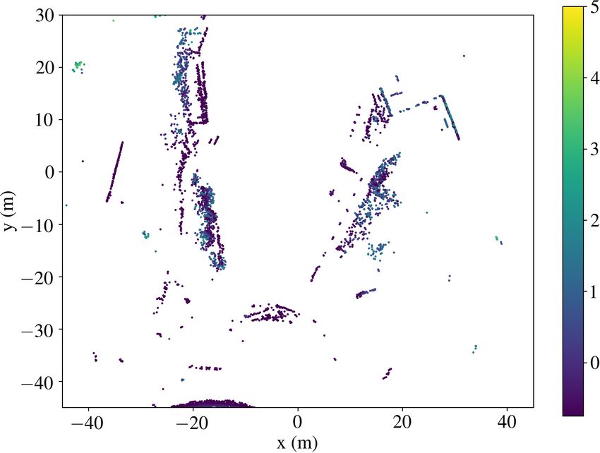
niques such as Constant False Alarm Rate (CFAR) [14] have
proven to be difficult to tune for radar-based localization.
Setting the threshold too high results in insufficient features,
which can cause localization to fail. Setting the threshold
too low results in a noisy radar pointcloud and a registration
process that is susceptible to local minima.
   Several promising methods have been proposed to improve
radar-based localization. Jose and Adams [15] demonstrated
a feature detector that estimates the probability of target
presence while augmenting their Simultaneous Localization
and Mapping (SLAM) formulation to include radar cross
section as an additional discriminating feature. Chandran
and Newman [16] maximized an estimate of map quality
to recover both the vehicle motion and radar map. Rou-
                                                                   Fig. 2.   The 8km Glen Shields route3 in Toronto. The yellow stars
veure et al. [17] and Checchin et al. [18] eschewed sparse         correspond to UTIAS, Dufferin, and Glen Shields (left to right) as in
feature extraction entirely by matching dense radar scans          Figure 5.
using 3D cross-correlation and the Fourier-Mellin transform.
Callmer et al. [19] demonstrated large-scale radar SLAM            The resulting radar pointclouds are registered to a sliding
by leveraging vision-based feature descriptors. Mullane et         window of keyframes using an Iterative Closest Point (ICP)-
al. [20] proposed to use a random-finite-set formulation of        like optimizer while accounting for motion distortion.
SLAM in situations of high clutter and data association               Other related work has focused on localizing radar scans
ambiguity. Vivet et al. [21] and Kellner et al. [9] proposed to    to satellite imagery [44]–[46], or to pre-built lidar maps [47],
use relative Doppler velocity measurements to estimate the         [48]. Localizing live radar scans to existing lidar maps built
instantaneous motion. Schuster et al. [22] demonstrated a          in ideal conditions is a desirable option as we still benefit
landmark-based radar SLAM that uses their Binary Annular           from the robustness of radar without incurring the expense of
Statistics Descriptor to match keypoints. Rapp et al. [23]         building brand new maps. However, the global localization
used Normalized Distributions Transform (NDT) to perform           errors reported in these works are in the range of 1m or
probabilistic ego-motion estimation with radar.                    greater. We demonstrate that we can successfully localize live
   Cen and Newman [24] demonstrated low-drift radar odom-          radar scans to a pre-built lidar map with a relative localization
etry over a large distance that inspired a resurgence of           error of around 0.1m.
research into radar-based localization. Several datasets have         In this work, we implement topometric localization that
been created to accelerate research in this area including         follows the Teach and Repeat paradigm [49], [50] without
the Oxford Radar RobotCar dataset [25], MulRan [26], and           using GPS or IMU measurements. Hong et al. [40] recently
RADIATE [27]. We have recently released our own dataset,           compared the performance of their radar SLAM to SuMa,
the Boreas dataset1 , which includes over 350km of data            surfel-based lidar SLAM [3]. On the Oxford RobotCar
collected on a repeated route over the course of 1 year.           dataset [25], they show that SuMa outperforms their radar
   More recent work in radar-based localization has fo-            SLAM. However, in their experiments, SuMa often fails
cused on either improving aspects of radar odometry [10],          partway through a route. Our interpretation is that SuMa
[28]–[37], developing better SLAM pipelines [38]–[40],             losing track is more likely due to an implementation detail
or performing place recognition [41]–[43]. Barnes et al.           inherent to SuMa itself rather than a shortcoming of all
[31] trained an end-to-end correlation-based radar odometry        lidar-based SLAM systems. It should be noted that Hong
pipeline. Barnes and Posner [32] demonstrated radar odom-          et al. did not tune SuMa beyond the original implementation
etry using deep learned features and a differentiable singular     which was tested on a different dataset. In addition, Hong
value decomposition (SVD)-based estimator. In [34], we             et al. tested SuMa using 32-beam lidar whereas the original
quantified the importance of motion distortion in radar odom-      implementation used a 64-beam lidar. Furthermore, Hong et
etry and showed that Doppler effects should be removed             al. only provide a qualitative comparison between their radar
during mapping and localization. Subsequently, in [35], we         SLAM and SuMA in rain, fog, and snow whereas our work
demonstrated unsupervised radar odometry, which combined           provides a quantitative comparison across varying weather
a learned front-end with a classic probabilistic back-end.         conditions. In some of the qualitative results they presented,
   Alhashimi et al. [37] present the current state of the art      it is unclear whether SuMa failed due to adverse weather or
in radar odometry. Their method builds on prior work by            due to geometric degeneracy in the environment which is a
Adolfsson et al. [36] by using a feature extraction algorithm      separate problem. Importantly, our results seem to conflict
called Bounded False Alarm Rate (BFAR) to add a constant           with theirs by showing that lidar localization can operate
offset b to the usual CFAR threshold: T = a · Z + b.               successfully in even moderate to heavy snowfall. Although,
                                                                   it is possible that topometric localization is more robust to
  1 https://www.boreas.utias.utoronto.ca/                          adverse weather since it uses both odometry and localization
  3 https://youtu.be/Cay6rSzeo1E/                                  to a pre-built map constructed in nominal weather.
III. METHODOLOGY T̂rk
A. Lidar/Radar Teach and Repeat Overview Fk=0 ... ... Fk Fr
Teach and Repeat is an autonomous route following frame-
work that manually teaches a robot a network of traversable (a) Teach Pass
paths [49], [51], [52]. A key enabling idea is the construction
of a topometric map [53] of the taught paths, represented T̂rk
as a pose graph in Figure 3. In the teach pass, a sequence Fk=0 ... Fk 0 ... Fk Fr
of sensor data (i.e., lidar or radar) from a driven route is
processed into local submaps stored along the path (vertices), Ťrm T̂rm
and are connected together by relative pose estimates (edges).
In the repeat pass, a new sequence of sensor data following Fm=0 ... Fm0 ... Fm
the same route is processed into a new branch of the
pose graph while simultaneously being localized against the
(b) Repeat Pass
vertices of the previous sequence to account for odometric
drift. By localizing against local submaps along the taught Fig. 3. The structure of the pose graph during (a) the teach pass and
paths, the robot can accurately localize and route-follow (b) the repeat pass. Fr is the moving robot frame and others are vertex
frames. We use subscript k for vertex frames from the current pass (teach
without the need for an accurate global reconstruction. In or repeat) and m for vertex frames from the reference pass (always teach).
this paper, we focus on the estimation pipeline of Teach and During both teach and repeat passes, we estimate the transformation from
Repeat (Figure 4). We divide the pipeline into: Preprocess- the latest vertex frame Fk to the robot frame Fr , T̂rk , using odometry.
For repeat passes only, we define Fk0 to be the latest vertex frame that has
ing, Odometry and Mapping, and Localization been successfully localized to the reference pass, Fm0 the corresponding
1) Preprocessing: This module performs feature extrac- map vertex of Fk0 , and Fm the spatially closest map vertex to Fr . A
tion and filtering on raw sensor data, which in our work prior estimate of the transform from Fm to Fr , Ťrm , is generated by
compounding transformations through Fm0 , Fk0 , and Fk , which is then
is from either lidar or radar sensors. More sensor-specific
used to compute the posterior T̂rm .
information is provided in III-B.
2) Odometry and Mapping: During both teach and repeat
passes, this module estimates the transformation between the as well as their covariances. We present the details of the
submap of the latest (local) vertex frame, Fk , and the latest ICP optimization in Section III-D.
live sensor scan at the current moving robot frame, Fr (i.e.,
T̂rk in Figure 3(a)). If the translation or rotation of T̂rk B. Raw Data Preprocessing
exceeds a predefined threshold (10m / 30 degrees), we add a 1) Lidar: For each incoming lidar scan, we first perform
new vertex Fk+1 connected with a new edge Tk+1,k = T̂rk . voxel downsampling with voxel size dl = 0.3m. Only one
Each edge consists of both the mean relative pose and its point that is closest to the voxel center is kept. Next, we
covariance (uncertainty) estimate. The new submap stored at extract plane features from the downsampled pointcloud by
Fk+1 is an accumulation of the last n = 3 processed sensor applying Principle Component Analysis (PCA) to each point
scans. All submaps are motion compensated and stored in and its neighbors from the raw scan. We define a feature
their respective (local) vertex frame. The live scan is also score from PCA to be
motion compensated and sent as input to the Localization
module. We present the details of our motion-compensated s = 1 − λmin /λmax , (3)
odometry algorithm, Continuous-Time Iterative Closest Point
where λmin and λmax are the minimum and maximum eigen-
(CT-ICP), in Section III-C.
values, respectively. The downsampled pointcloud is then
3) Localization: During the repeat pass, this module
filtered by this score, keeping no more than 20,000 points
localizes the motion-compensated live scan of the robot
with scores above 0.95. We associate each point with its
frame, Fr , against the submap of the spatially closest vertex
eigenvector of λmin from PCA as the underlying normal.
frame, Fm , of the previous sequence (i.e., T̂rm as shown
2) Radar: For each radar scan, we first extract point
in Figure 3(b)). Vertex frame Fm is chosen by leveraging
targets from each azimuth using the Bounded False Alarm
our latest odometry estimate and traversing through the pose
Rate (BFAR) detector as described in [37]. BFAR adds a con-
graph edges. Given the pose graph in Figure 3(b), the initial
stant offset b to the usual Cell-Averaging CFAR threshold:
estimate to Fm is
T = a·Z +b. We use the same (a, b) parameters as [37]. For
Ťrm = Trk Tkk0 Tk0 m0 Tm0 m . (1) each azimuth, we also perform peak detection by calculating
the centroid of contiguous groups of detections as is done
We localize using ICP with Ťrm as a prior, resulting in
in [24]. We obtained a modest performance improvement by
T̂rm . If ICP alignment is successful, we add a new edge
retaining the maximum of the left and right sub-windows
between the vertex of Fm and the latest vertex of the current
relative to the cell under test as in (greatest-of) GO-CFAR
sequence, Fk , by compounding the mean localization result
[14]. These polar targets are then transformed into Cartesian
with the latest odometry result,
coordinates and are passed to the Odometry and Mapping
T̂km = T̂−1
rk T̂rm , (2) module without further filtering.Preprocessing Odometry and Mapping Localization
Fk Fm
Submap Submap
Radar/Lidar Feature Map
Filtering Registration Registration
Input Extraction Maintenance
Fk+1
T̂rk Submap T̂rm
Fig. 4. The data processing pipeline of our Teach and Repeat implementation, divided into three modules: Preprocessing, Odometry and Mapping, and
Localization. See III-A for a detailed description of each module.
C. Continuous-Time ICP and expressed in Fk , and D is a constant projection that
Our odometry algorithm, CT-ICP, combines the iterative removes the 4th homogeneous element. We define R−1 j as
data association of ICP with a continuous-time trajectory either a constant diagonal matrix for radar data (point-to-
represented as exactly sparse Gaussian Process regression point) or by using the outer product of the corresponding
[54]. Our trajectory is x(t) = {T(t), $(t)}, where T(t) ∈ surface normal estimate for lidar data (point-to-plane).
SE(3) is our robot pose and $(t) ∈ R6 is the body- We optimize for xi = {Ti , $ i } iteratively using Gauss-
centric velocity. Following Anderson and Barfoot [54], our Newton, but with nearest-neighbours data association af-
GP motion prior is ter every Gauss-Newton iteration. CT-ICP is therefore per-
formed with the following steps:
Ṫ(t) = $(t)∧ T(t), 1) Temporarily transform all points qj to frame Fk using
(4)
$̇ = w(t), w(t) ∼ GP(0, Qc δ(t − τ )), the latest trajectory estimate (motion undistortion).
2) Associate each point to its nearest neighbour in the
where w(t) ∈ R6 is a zero-mean, white-noise Gaussian
map to identify its corresponding map point pjk in Fk .
process, and the operator, ∧, transforms an element of R6
3) Formulate the cost function J in (5) and perform a
into a member of Lie algebra, se(3) [55].
single Gauss-Newton iteration to update Ti and $ i .
The prior (4) is applied in a piecewise fashion between
4) Repeat steps 1 to 3 until convergence.
an underlying discrete trajectory of pose-velocity state pairs,
xi = {Ti , $ i }, that each correspond to the representative The output of CT-ICP at the timestamp of the latest sensor
timestamp of the ith sensor scan. Each pose, Ti , is the scan is then the odometry output T̂r,k .
relative transform from the latest vertex, Fk , to the robot D. Localization ICP
frame, Fr , that corresponds to the ith sensor scan (i.e., Trk ). We use ICP to localize the motion-compensated live
Likewise, $ i is the corresponding body-centric velocity. We scan of the robot frame, Fr , against the submap of the
seek to align the latest sensor scan i to the latest vertex spatially closest vertex frame, Fm , of the previous sequence.
submap in frame Fk (see Figure 3). The resulting relative transformation is T̂rm , as shown in
We define a nonlinear optimization for the latest state xi , Figure 3(b). The nonlinear cost function is
locking all previous states. The cost function is M
X 1 T
M
1 T
Jloc = φpose + eloc,j R−1
j eloc,j , (7)
2
X
−1
Jodom = φmotion + e R eodom,j . (5)
2 odom,j j
j=1
j=1
| {z } where we use Ťrm from (1) as an initial guess and a prior:
measurements
1 ∨ T −1
In the interest of space, we refer readers to Anderson and φpose = ln(Ťrm T−1 rm ) Qrm ln(Ťrm T−1 ∨
rm ) , (8)
2
Barfoot [54] for the squared-error cost expression of the where ln (·) is the logarithm map and the operator ∨ is the
motion prior, φmotion . Each measurement error term is inverse of ∧ [55]. The covariance Qrm can be computed
by compounding the edge covariances corresponding to the
eodom,j = D pjk − T(tj )−1 Trs qj , (6)
relative transformations in (1). Since all pointclouds are
where qj is a homogeneous point with corresponding times- already motion-compensated, the measurement error term is
tamp tj from the ith sensor scan, Trs is the extrinsic simply
calibration from the sensor frame Fs to the robot frame Fr , eloc,j = D pjm − T−1 (9)
rm Trs qj ,
T(tj ) is a pose from our trajectory queried at tj 4 , pjk is a
where qj is a homogeneous point from the motion-
homogeneous point from the kth submap associated to qj
compensated live scan, and pjm is the nearest neighbour
4 Through interpolation, T(t ) depends on the state variables x =
j i
submap point to qj . See Section III-C for how we define
{Ti , $ i } and xi−1 = {Ti−1 , $ i−1 } since tj > ti−1 [54]. Trs , D, and R−1
j .Teach Repeats
UTIAS
Glen Shields Dufferin 2020-11-26 2020-12-04 2021-01-26 2021-02-09 2021-03-09 2021-06-29 2021-09-08
Fig. 5. Our test sequences were collected by driving a repeated route over the source of one year. In our experiments, we use 2020-11-26 as our reference
sequence for building maps. The remaining six sequences, which include sequences with rain and snow, are used to benchmark localization performance,
which amounts to 48km of test driving. These camera images are provided for context.
Lateral Error (m) Longitudinal Error (m) Heading Error (deg)
0.5
Lidar-to-Lidar
0.6 0.6 0.6
Lidar-to-Lidar
0.4 0.4 0.4 0.0
0.2 0.2 0.2 −0.5
0 200 400 600 800 1000 1200
0.0 0.0 0.0
0.5
Radar-to-Radar
−1.00 0.00 1.00 −1.00 0.00 1.00 −2.0 0.0 2.0
0.4 0.4 0.4
0.0
Radar-to-Radar
0.2 0.2 0.2 −0.5
0 200 400 600 800 1000 1200
0.5
Radar-to-Lidar
0.0 0.0 0.0
−1.00 0.00 1.00 −1.00 0.00 1.00 −2.0 0.0 2.0
0.0
0.4 0.4 0.4
Radar-to-Lidar
−0.5
0.2 0.2 0.2 0 200 400 600 800 1000 1200
Time (s)
Lateral Error (m) Longitudinal Error (m)
0.0 0.0 0.0
−1.00 0.00 1.00 −1.00 0.00 1.00 −2.0 0.0 2.0
Fig. 7. Here we plot metric localization errors during the snowstorm
Fig. 6. These histograms show the spread of the localization error for lidar-
sequence 2021-01-26. Note that the lidar localization estimates remain
to-lidar, radar-to-radar, and radar-to-lidar, during the snowstorm sequence
accurate even with 1/4 of its field of view being blocked by a layer of
2021-01-26.
ice as shown in Figure 9.
E. Doppler-Compensated ICP
eodom,j = D pjk − T(tj )−1 Trs (qj + ∆qj ) (10)
In our prior work [34], we showed that current Navtech
where ∆qj = DT βaj aTj Dqj Ad(Tsr )$(tj ), (11)
radar sensors are susceptible to Doppler distortion and that
this effect becomes significant during mapping and local- β is Doppler distortion constant inherent to the sensor [34],
ization. A relative velocity between the sensor and the and aj is a 3 × 1 unit vector in the direction of qj . The
surrounding environment causes the received frequency to operator allows one to swap the order of the operands
be altered according to the Doppler effect. If the velocity in associated with the ∧ operator [55]. Ad(·) represents the
the sensor frame is known, this effect can be compensated adjoint of an element of SE(3) [55].
for using a simple additive correction factor ∆qj . In this
work, we include this correction factor, which depends on a IV. E XPERIMENTAL R ESULTS
continuous-time interpolation of the estimated body-centric In this section, we compare the performance of radar-
velocity $(t) at the measurement time of each target tj , in only, lidar-only, and radar-to-lidar topometric localization.
the measurement error term for radar CT-ICP: Our experimental platform, depicted in Figure 1, includes60
snow
40
20
y (m)
0
−20
−40
−60
−60 −40 −20 0 20 40 60
x (m)
(a) Radar-to-Radar (a) Lidar with snow detections
60
40
20
y (m)
0
−20
−40
−60 −40 −20 0 20 40
x (m)
(b) Lidar with outliers removed
(b) Radar-to-Lidar
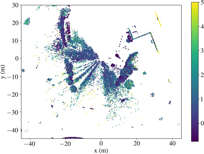
Fig. 9. This figure illustrates the noisy lidar data that was used to localize
Fig. 8. This figure shows the live radar pointcloud (blue) registered to a during the 2021-01-26 sequence. Points are colored by their z-height. In (a)
submap (red) built during the teach pass. In (a) we are performing radar-to- the ground plane has been removed and the pointcloud has been randomly
radar localization and so the submap is made up of radar points. In (b) we downsampled by 50% to highlight the snowflake detections. Note that a
are localizing a radar pointcloud (blue) to a previously built lidar submap. large forward section of the lidar’s field of view is blocked by a layer of
ice. However, as the results in Table I and Figure 7 show, lidar localization
remains quite robust under these adverse conditions. (b) shows the lidar
pointcloud after filtering points by their normal score as in Equation 3 and
a 128-beam Velodyne Alpha-Prime lidar, a FLIR Blakfly only retaining the inliers of truncated least squares. Note that the snowflake
detections seem to disappear, illustrating the robustness of our lidar pipeline.
S monocular camera, a Navtech radar, and an Applanix
POS LV GNSS-INS. Our lidar has a 40◦ vertical field of
view, 0.1◦ vertical angular resolution, 0.2◦ horizontal angular
resolution, and produces roughly 220k points per revolution the map. No GPS or IMU information is required during the
at 10Hz up to 300m. The Navtech is a frequency modulated map-building process. Note that our test sequences include
continuous wave (FMCW) radar with a 0.9◦ horizontal angu- a significant amount of seasonal variation with ten months
lar resolution and 5.96cm range resolution, which provides separating the initial teach pass and the final repeat pass.
measurements up to 200m at 4Hz. The test sequences used in Sequences 2021-06-29 and 2021-09-08 include trees with
this paper are part of our new Boreas dataset, which contains full foliage while the remaining sequences lack this. 2021-
over 350km of driving data collected by driving a repeated 01-26 was collected during a snowstorm, 2021-06-29 was
route over the course of one year [7]. Ground truth poses are collected in the rain, and 2021-09-08 was collected at night.
obtained by post-processing GNSS, IMU, and wheel encoder During each of the repeat traversals, our topometric lo-
measurements. An RTX subscription was used to achieve calization outputs a relative localization estimate between
cm-level accuracy without a base station. RTX uses data from the live sensor frame s2 and a sensor frame in the map s1 :
a global network of tracking stations to calculate corrections. T̂s1 ,s2 . We then compute root mean squared error (RMSE)
The residual error of the post-processed poses reported by values for the relative translation and rotation error as in [7].
Applanix is typically 2-4cm in nominal conditions. We separate translational error into lateral and longitudinal
In this experiment, we used seven sequences of the Glen components. Since the Navtech radar is a 2D sensor, we
Shields route (shown in Figure 2) chosen for their distinct restrict our comparison to SE(2) by omitting z errors and
weather conditions.. These sequences are depicted in Fig- reporting heading error as the rotation error.
ure 5. During the teach pass, a map is constructed using the Figure 6 depicts the spread of localization error during
reference sequence 2020-11-26. The radar-only and lidar- sequence 2021-01-26. Note that, although lidar-to-lidar lo-
only pipelines use their respective sensor types to construct calization is the most accurate, radar-to-radar localizationTABLE I
remains reasonably competitive. When localizing radar scans M ETRIC L OCALIZATION RMSE R ESULTS
to lidar maps, both the longitudinal error and heading error R EFERENCE S EQUENCE : 2020-11-26
incur a bias. The longitudinal bias could be due to some
Lidar-to-Lidar
residual Doppler distortion effects, and the heading bias lateral (m) longitudinal (m) heading (deg)
could be the result of an error in the radar-to-lidar extrinsic 2020-12-04 0.057 0.082 0.025
calibration. A video showcasing radar mapping and localiza- 2021-01-26 0.047 0.034 0.034
2021-02-09 0.044 0.037 0.029
tion can be found at this link5 . 2021-03-09 0.049 0.040 0.022
Figure 7 shows the localization errors as a function of time 2021-06-29 0.052 0.058 0.042
during the snowstorm sequence 2021-01-26. Surprisingly, 2021-09-08 0.060 0.041 0.030
mean 0.052 0.049 0.030
lidar localization appears to be unperturbed by the adverse
Radar-to-Radar
weather conditions. During the snowstorm sequence, the lateral (m) longitudinal (m) heading (deg)
lidar pointcloud becomes littered with detections associated 2020-12-04 0.130 0.127 0.223
with snowflakes and a large section of the horizontal field 2021-01-26 0.118 0.098 0.201
2021-02-09 0.111 0.089 0.203
of view becomes blocked by a layer of ice as shown in 2021-03-09 0.129 0.093 0.213
Figure 9 (a). However, in Figure 9 (b), we show that in 2021-06-29 0.163 0.155 0.241
actuality, these snowflake detections have little impact on 2021-09-08 0.155 0.148 0.231
ICP registration after filtering by normal score and only mean 0.134 0.118 0.219
retaining the inliers of truncated least squares. Charron et Radar-to-Lidar
lateral (m) longitudinal (m) heading (deg)
al. [56] previously demonstrated that snowflake detections 2020-12-04 0.132 0.179 0.384
can be removed from lidar pointclouds, although we do not 2021-01-26 0.130 0.153 0.360
use their method here. The robustness of our lidar pipeline 2021-02-09 0.126 0.152 0.389
2021-03-09 0.140 0.152 0.360
to both weather and seasonal variations is reflected in the 2021-06-29 0.159 0.161 0.415
RMSE results displayed in Table I. 2021-09-08 0.169 0.165 0.401
Our results show that, contrary to the assertions made mean 0.143 0.161 0.385
by prior works, lidar localization can be robust to moderate TABLE II
levels of precipitation and seasonal variation. Clearly, more C OMPUTATIONAL AND S TORAGE R EQUIREMENTS
work is required by the community to identify operational
conditions where radar localization has a clear advantage. Odom. Loc. Storage
These conditions may include very heavy precipitation, dense (FPS) (FPS) (MB/km)
Lidar-to-Lidar 3.6 3.0 86.4
fog, or dust clouds. Nevertheless, we demonstrated that Radar-to-Radar 5.3 5.1 5.6
our radar localization is reasonably competitive with lidar. Radar-to-Lidar N/A 5.1 86.4
Furthermore, radar localization may still be important as a
redundant backup system in autonomous vehicles. Figure 8
illustrates the live scan and submap during radar-to-radar and We used a Lenovo P53 laptop with Intel(R) Core(TM) i7-
radar-to-lidar localization. 9750H CPU @ 2.60GHz and 32GB of memory. A GPU was
It is important to recognize that the results reported in this not used. Our radar-based maps use significantly less storage
work are taken at a snapshot in time. Radar localization is (5.6MB/km) than our lidar-based maps (86.4MB/km).
not as mature of a field as lidar localization and radar sensors V. CONCLUSIONS
themselves still have room to improve. Note that incorporat-
ing IMU or wheel encoder measurements would improve the In this work, we compared the performance of lidar-to-
performance of all three compared systems. The detector we lidar, radar-to-radar, and radar-to-lidar topometric localiza-
used, BFAR [37], did not immediately work when applied tion. Our results showed that radar-based pipelines are a
to a new radar with different noise characteristics. It is viable alternative to lidar localization but lidar continues to
possible that a learning-based approach to feature extraction yield the best results. Surprisingly, our experiments showed
and matching may improve performance. Switching to a that lidar-only mapping and localization is quite robust to
landmark-based pipeline or one based on image correlation adverse weather such as a snowstorm with a partial sensor
may also be interesting avenues for comparison. blockage due to ice. We identified several areas for future
Radar-to-lidar localization is attractive because it allows work and noted that more experiments are needed to identify
us to use existing lidar maps, which many autonomous conditions where the performance of radar-based pipelines
driving companies already have, while taking advantage of exceeds that of lidar.
the robustness of radar sensing. Radar-based maps are not R EFERENCES
as useful as lidar maps since they lack sufficient detail to be [1] J. Levinson and S. Thrun, “Robust vehicle localization in urban
used to create semantic maps. environments using probabilistic maps,” in ICRA. IEEE, 2010.
In Table II, we show the computational and storage [2] R. W. Wolcott and R. M. Eustice, “Fast lidar localization using
multiresolution gaussian mixture maps,” in ICRA. IEEE, 2015.
requirements of the different pipelines discussed in this work. [3] J. Behley and C. Stachniss, “Efficient surfel-based slam using 3d laser
range data in urban environments.” in Robotics: Science and Systems,
5 https://youtu.be/okS7pF6xX7A 2018.[4] M. Gridseth and T. D. Barfoot, “Keeping an eye on things: Deep [30] ——, “Fast radar motion estimation with a learnt focus of attention
learned features for long-term visual localization,” RA-L, 2021. using weak supervision,” in ICRA. IEEE, 2019.
[5] G. M. Brooker, S. Scheding, M. V. Bishop, and R. C. Hennessy, [31] D. Barnes, R. Weston, and I. Posner, “Masking by moving: Learning
“Development and application of millimeter wave radar sensors for distraction-free radar odometry from pose information,” in Conference
underground mining,” IEEE Sensors journal, vol. 5, no. 6, pp. 1270– on Robot Learning, 2020.
1280, 2005. [32] D. Barnes and I. Posner, “Under the radar: Learning to predict robust
[6] G. Brooker, M. Bishop, and S. Scheding, “Millimetre waves for keypoints for odometry estimation and metric localisation in radar,”
robotics,” in Australian Conference for Robotics and Automation, in ICRA. IEEE, 2020.
2001. [33] Y. S. Park, Y.-S. Shin, and A. Kim, “Pharao: Direct radar odometry
[7] K. Burnett, D. J. Yoon, Y. Wu, A. Z. Li, H. Zhang, S. Lu, J. Qian, using phase correlation,” in ICRA, 2020.
W.-K. Tseng, A. Lambert, K. Y. Leung, A. P. Schoellig, and T. D. [34] K. Burnett, A. P. Schoellig, and T. D. Barfoot, “Do we need to
Barfoot, “Boreas: A multi-season autonomous driving dataset,” arXiv compensate for motion distortion and doppler effects in spinning radar
preprint arXiv:2203.10168, 2022. navigation?” RA-L, 2021.
[8] H. Caesar, V. Bankiti, A. H. Lang, S. Vora, V. E. Liong, Q. Xu, [35] K. Burnett, D. J. Yoon, A. P. Schoellig, and T. D. Barfoot, “Radar
A. Krishnan, Y. Pan, G. Baldan, and O. Beijbom, “nuscenes: A odometry combining probabilistic estimation and unsupervised feature
multimodal dataset for autonomous driving,” in CVPR, 2020. learning,” in Robotics: Science and Systems, 2021.
[9] D. Kellner, M. Barjenbruch, J. Klappstein, J. Dickmann, and K. Diet- [36] D. Adolfsson, M. Magnusson, A. Alhashimi, A. J. Lilienthal, and
mayer, “Instantaneous ego-motion estimation using doppler radar,” in H. Andreasson, “Cfear radarodometry-conservative filtering for effi-
ITSC. IEEE, 2013. cient and accurate radar odometry,” in IROS. IEEE, 2021.
[10] P.-C. Kung, C.-C. Wang, and W.-C. Lin, “A normal distribution [37] A. Alhashimi, D. Adolfsson, M. Magnusson, H. Andreasson, and A. J.
transform-based radar odometry designed for scanning and automotive Lilienthal, “Bfar-bounded false alarm rate detector for improved radar
radars,” in ICRA. IEEE, 2021. odometry estimation,” arXiv preprint arXiv:2109.09669, 2021.
[38] M. Holder, S. Hellwig, and H. Winner, “Real-time pose graph slam
[11] P. Gao, S. Zhang, W. Wang, and C. X. Lu, “Accurate automotive radar
based on radar,” in IV. IEEE, 2019.
based metric localization with explicit doppler compensation,” arXiv
[39] Z. Hong, Y. Petillot, and S. Wang, “Radarslam: Radar based large-
preprint arXiv:2112.14887, 2021.
scale slam in all weathers,” in IROS. IEEE, 2020.
[12] S. Clark and H. Durrant-Whyte, “Autonomous land vehicle navigation
[40] Z. Hong, Y. Petillot, A. Wallace, and S. Wang, “Radarslam: A
using millimeter wave radar,” in ICRA. IEEE, 1998.
robust simultaneous localization and mapping system for all weather
[13] M. G. Dissanayake, P. Newman, S. Clark, H. F. Durrant-Whyte, and conditions,” IJRR, 2022.
M. Csorba, “A solution to the simultaneous localization and map [41] D. De Martini, M. Gadd, and P. Newman, “kradar++: Coarse-to-fine
building (slam) problem,” T-RO, 2001. fmcw scanning radar localisation,” Sensors, 2020.
[14] H. Rohling, “Radar cfar thresholding in clutter and multiple target [42] Ş. Săftescu, M. Gadd, D. De Martini, D. Barnes, and P. Newman,
situations,” IEEE transactions on aerospace and electronic systems, “Kidnapped radar: Topological radar localisation using rotationally-
1983. invariant metric learning,” in ICRA. IEEE, 2020.
[15] E. Jose and M. D. Adams, “Relative radar cross section based feature [43] M. Gadd, D. De Martini, and P. Newman, “Look around you:
identification with millimeter wave radar for outdoor slam,” in IROS. Sequence-based radar place recognition with learned rotational invari-
IEEE, 2004. ance,” in PLANS, 2020.
[16] M. Chandran and P. Newman, “Motion estimation from map quality [44] T. Y. Tang, D. De Martini, D. Barnes, and P. Newman, “Rsl-net:
with millimeter wave radar,” in IROS. IEEE, 2006. Localising in satellite images from a radar on the ground,” RA-L,
[17] R. Rouveure, M. Monod, and P. Faure, “High resolution mapping of 2020.
the environment with a ground-based radar imager,” in RADAR. IEEE, [45] T. Y. Tang, D. De Martini, S. Wu, and P. Newman, “Self-supervised lo-
2009. calisation between range sensors and overhead imagery,” in Robotics:
[18] P. Checchin, F. Gérossier, C. Blanc, R. Chapuis, and L. Trassoudaine, Science and Systems, 2020.
“Radar scan matching slam using the fourier-mellin transform,” in [46] T. Y. Tang, D. De Martini, and P. Newman, “Get to the point:
FSR. Springer, 2010. Learning lidar place recognition and metric localisation using overhead
[19] J. Callmer, D. Törnqvist, F. Gustafsson, H. Svensson, and P. Carlbom, imagery,” in Robotics: Science and Systems, 2021.
“Radar slam using visual features,” EURASIP Journal on Advances in [47] H. Yin, Y. Wang, L. Tang, and R. Xiong, “Radar-on-lidar: metric
Signal Processing, 2011. radar localization on prior lidar maps,” in 2020 IEEE International
[20] J. Mullane, B.-N. Vo, M. D. Adams, and B.-T. Vo, “A random-finite-set Conference on Real-time Computing and Robotics (RCAR). IEEE,
approach to bayesian slam,” T-RO, 2011. 2020.
[21] D. Vivet, P. Checchin, and R. Chapuis, “Localization and mapping [48] H. Yin, R. Chen, Y. Wang, and R. Xiong, “Rall: end-to-end radar
using only a rotating fmcw radar sensor,” Sensors, 2013. localization on lidar map using differentiable measurement model,”
[22] F. Schuster, C. G. Keller, M. Rapp, M. Haueis, and C. Curio, IEEE Transactions on Intelligent Transportation Systems, 2021.
“Landmark based radar slam using graph optimization,” in ITSC. [49] P. Furgale and T. D. Barfoot, “Visual teach and repeat for long-range
IEEE, 2016. rover autonomy,” JFR, 2010.
[23] M. Rapp, M. Barjenbruch, M. Hahn, J. Dickmann, and K. Dietmayer, [50] M. Paton, K. MacTavish, M. Warren, and T. D. Barfoot, “Bridging
“Probabilistic ego-motion estimation using multiple automotive radar the appearance gap: Multi-experience localization for long-term visual
sensors,” Robotics and Autonomous Systems, 2017. teach and repeat,” in IROS, 2016.
[24] S. H. Cen and P. Newman, “Precise ego-motion estimation with [51] M. Paton, K. MacTavish, L.-P. Berczi, S. K. van Es, and T. D. Barfoot,
millimeter-wave radar under diverse and challenging conditions,” in “I can see for miles and miles: An extended field test of visual teach
ICRA. IEEE, 2018. and repeat 2.0,” in FSR. Springer, 2018.
[25] D. Barnes, M. Gadd, P. Murcutt, P. Newman, and I. Posner, “The [52] P. Krüsi, B. Bücheler, F. Pomerleau, U. Schwesinger, R. Siegwart, and
oxford radar robotcar dataset: A radar extension to the oxford robotcar P. Furgale, “Lighting-invariant adaptive route following using iterative
dataset,” in ICRA. IEEE, 2020. closest point matching,” JFR, 2015.
[53] H. Badino, D. Huber, and T. Kanade, “Visual topometric localization,”
[26] G. Kim, Y. S. Park, Y. Cho, J. Jeong, and A. Kim, “Mulran: Multi-
in IV, 2011.
modal range dataset for urban place recognition,” in ICRA. IEEE,
[54] S. Anderson and T. D. Barfoot, “Full steam ahead: Exactly sparse
2020.
gaussian process regression for batch continuous-time trajectory esti-
[27] M. Sheeny, E. De Pellegrin, S. Mukherjee, A. Ahrabian, S. Wang,
mation on se(3),” in IROS, 2015.
and A. Wallace, “Radiate: A radar dataset for automotive perception
[55] T. D. Barfoot, State Estimation for Robotics. Cambridge University
in bad weather,” in ICRA. IEEE, 2021.
Press, 2017.
[28] S. H. Cen and P. Newman, “Radar-only ego-motion estimation in [56] N. Charron, S. Phillips, and S. L. Waslander, “De-noising of lidar
difficult settings via graph matching,” in ICRA. IEEE, 2019. point clouds corrupted by snowfall,” in CRV. IEEE, 2018.
[29] R. Aldera, D. De Martini, M. Gadd, and P. Newman, “What could go
wrong? introspective radar odometry in challenging environments,” in
ITSC. IEEE, 2019.You can also read


