Applying spline-based phase analysis to macroeconomic dynamics
←
→
Page content transcription
If your browser does not render page correctly, please read the page content below
Dependence Modeling 2022; 10: 207–214
Research Article
Special Issue on Econometrics and Business Analytics
Gadasina Lyudmila*, Vyunenko Lyudmila
Applying spline-based phase analysis to
macroeconomic dynamics
https://doi.org/10.1515/demo-2022-0113
received September 01, 2021; accepted April 22, 2022
Abstract: The article uses spline-based phase analysis to study the dynamics of a time series of low-
frequency data on the values of a certain economic indicator. The approach includes two stages. At the
first stage, the original series is approximated by a smooth twice-differentiable function. Natural cubic
splines are used as an approximating function y . Such splines have the smallest curvature over the
observation interval compared to other possible functions that satisfy the choice criterion. At the second
stage, a phase trajectory is constructed in (t , y , y′)-space, corresponding to the original time series, and a
phase shadow as a projection of the phase trajectory onto the ( y , y′)-plane. The approach is applied to the
values of GDP indicators for the G7 countries. The interrelation between phase shadow loops and cycles of
economic indicators evolution is shown. The study also discusses the features, limitations and prospects for
the use of spline-based phase analysis.
Keywords: cubic spline, phase trajectory, phase shadow, dynamic system
MSC 2020: 65D15, 65D07, 37C50
1 Introduction
Traditionally, regression and autoregressive models are used to analyze the dynamics of macroeconomic
indicators. Such approaches require a priori definition of the model specification and rather strict assump-
tions about the data properties for example stationarity. Another approach is to consider the time series of
macroeconomic indicators as a function of the dynamic system states, it’s evolution being described by
deterministic or stochastic differential equations [5,6,9,10,11].
The values of macroeconomic indicators are aggregated and averaged over relatively long periods. This
allows us to consider them as deterministic ones and provides the basis for applying the second approach.
In this case, the main task is to reconstruct the dynamic system that generated the time series. According to
Takens’ theorem [8], a description of the phase space of a dynamical system can be obtained if, instead of
the real variables of the system, we take finite-dimensional delay vectors composed of the values series at
successive moments of time.
This study uses the approach called spline-based phase analysis to investigate a time series of low-
frequency data. It is applicable to the analysis of the macroeconomic indicators dynamics, such as GDP,
consumption, foreign trade balance, etc. Spline-based phase analysis can adequately assess the features of
the process, which remain unnoticed when using simple regression models.
* Corresponding author: Gadasina Lyudmila, Center for Econimetrics and Business Analytics (CEBA), St Petersburg State
University, 7-9, Universitetskaya nab., St Petersburg, 199034, Russian Federation, e-mail: l.gadasina@spbu.ru
Vyunenko Lyudmila: St Petersburg State University, 7-9, Universitetskaya nab., St Petersburg, 199034, Russian Federation,
e-mail: l.vyunenko@spbu.ru
Open Access. © 2022 Gadasina Lyudmila and Vyunenko Lyudmila, published by De Gruyter. This work is licensed under the
Creative Commons Attribution 4.0 International License.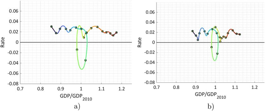
208 Gadasina Lyudmila and Vyunenko Lyudmila
The approach includes two stages. At the first one, we replace the discrete time series Yi of economic
indicators by a smooth function g (t ) that best approximates the original discrete time series according to a
certain criterion described later. The second stage consists in analyzing the joint behavior of the con-
structed function and it’s first derivative g ′(t ).
The criterion for choosing an approximating function is as follows. It should be continuous, adaptive
and provide a minimum error in the description of the data under study. The specified requirements are
simultaneously satisfied by interpolation cubic spline functions.
In a number of studies [1,2, 4,7], spline interpolation is effectively used to analyze low-frequency data.
For example, Chakroun and Abid state that “the cubic spline method is a tractable and reasonably correct
estimation method that we recommend in any market with infrequent trading” [2]. Roul and Prasad Goura
[7] demonstrate the effectiveness of using splines for the Asian option pricing problem. The authors
recommend using the cubic spline method to analyze stock quotes in any market with infrequent trading.
2 Data description and methodology
We consider historical annual data on GDP for G7 countries in 2000–2019. Data source is World Bank Group
– International Development, Poverty, & Sustainability [12].
The collected datasets have the following properties: the data are low-frequency and highly aggregated.
This means that it is free of noise and can be considered “as is.”
Note that the data source allows obtaining the indicator values under consideration in the homoge-
neous data format, i.e., the data are considered in the same units of measurement for the entire period of the
study. This is important both for economic analysis and for correct approximation of the examined time
series. Therefore, we consider the indicators at constant prices (constant 2010 US$).
To study the behavior of the indicator time series, it is necessary to construct its approximation, which
has the following properties: it is a twice continuously differentiable function with the graph connecting the
given values of a series by the curve of the minimal length.
Thus, we solve the interpolation problem. As an interpolant, we consider a one-dimensional cubic
spline g (t ), which is defined as follows.
Given a set of n + 1 data points (ti, yi ), i = 1, 2, … , n , where ti are time moments, a = t0 < t1 < ⋯ < tn = b.
The spline g (t ) is a function satisfying: g (t ) ∈ C2[a , b].
On subinterval [ti − 1, ti], i = 0, … , n, function g (t ) = gi (t ) is a polynomial of degree 3, g (ti ) = yi ,
i = 0, … , n.
Common form of notation using the coefficients of the polynomials:
3
gi (t ) = ∑ ai(k )(t − ti−1)k .
k=0
The constructing of an interpolation cubic spline is reduced to solving a system of linear algebraic
equations (with respect to the coefficients of piecewise polynomials or the node slopes). To receive a
uniquely solvable system, two additional equations are necessary. These equations are obtained from
the specified boundary conditions. The most common are the following options:
• Natural spline, which meets the boundary conditions:
g1″(t0) = gn″(tn) = 0.
• Not-a-knot spline, which meets the boundary conditions
g1‴(t1) = g2‴(t1) ,
gn‴− 1(tn − 1) = gn‴(tn − 1) .
Holladay’s theorem is true for the natural spline [3].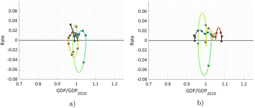
Applying spline-based phase analysis to macroeconomic dynamics 209
Theorem 1. (Holladay) If g (t ) – natural interpolation spline on [a , b] knots a = t0 < t1 < ⋯ < tn = b, f (t ) – any
function, then
E ( f ) ≥ E (g ) ,
where
b
E( f ) = ∫( f ″(t ))2dt ,
a
and the inequality is strict for f ≠ g .
For research purposes, it is important that the approximating function connects the known values by
the curve of minimum length. Taking into account Holladey’s theorem, we choose natural splines. Thus, the
constructed approximation allows replacing discrete values with a continuous smooth function. The study
of its behavior enables conclusions about the dynamics of changes in the indicators under consideration.
The second stage of the approach is related to the constructing of a phase trajectory and a phase
shadow. The concept of a phase trajectory is associated with the qualitative theory of differential equations,
in particular, with the visualization of solutions of ordinary differential equations. In the general case, a
phase shadow is a geometric representation of the dynamic system trajectories in the phase plane.
In our study, by the phase trajectory, we mean a curve in three-dimensional space (t , y , y′), where t –
observation time, y – values of the smoothing function, and y′ – the first derivative values of the smoothed
function. By the phase shadow, we mean the projection of the phase trajectory onto the plane ( y , y′). Phase
shadows enable illustrating the change in the behavior of the function under study in terms of its deviations
from the general trend, if any, and to show the stability of this trend.
3 Empirical results
To demonstrate how phase shadows allow analyzing the similarities and differences in the behavior of
macroeconomic indicators for different countries, we consider the values of the G7 countries (Germany,
France, Italy, Canada, USA, Japan) GDP over 2000–2019.
First, using the example of German GDP data, we consider the application of the outlined approach.
Figure 1 shows the GDP values for the period 2000–2019 and the graph of the corresponding natural
interpolating cubic spline gGer (t ).
Figure 1: GDP (bold points) and natural interpolating cubic spline graph (blue line) for Germany over 2000–2019.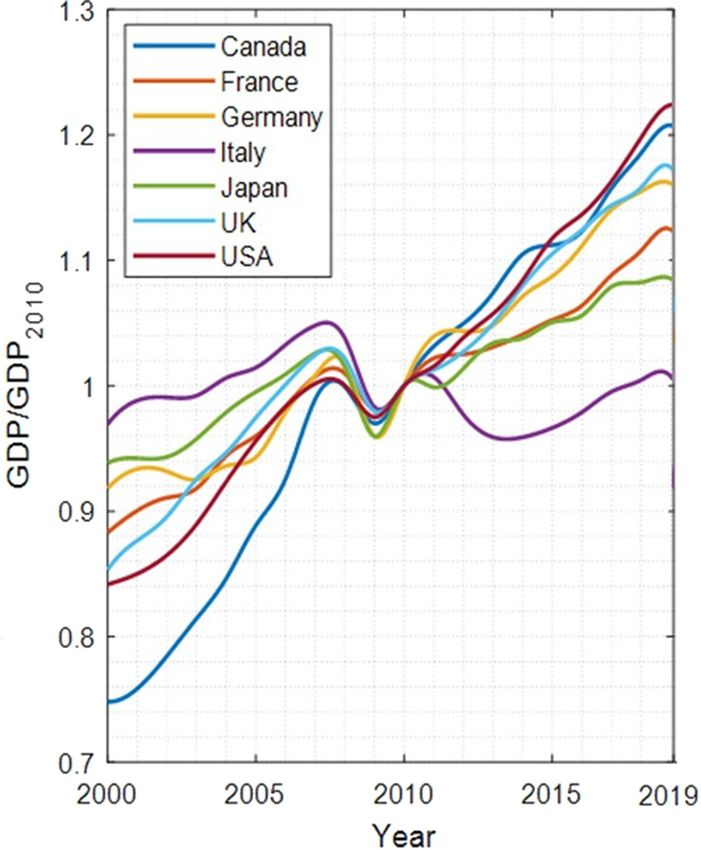
210 Gadasina Lyudmila and Vyunenko Lyudmila
Figure 2: The German GDP phase trajectory based on the spline approximation of statistical data over 2000–2019.
The approximating function being constructed, we obtain the opportunity to visualize a phase trajec-
tory (Figure 2) as a three-dimensional graph with the coordinate axes corresponding to time t in years, the
′ (t ) .
values of gGer (t ) and gGer
For the convenience of the analysis, a colorbar is used, which allows one to compare points on the
phase trajectory with a time period.
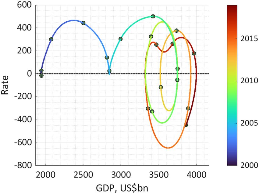
Figure 3 presents the phase shadow as a projection of the phase trajectory onto the plane (GDP, rate).
The phase shadow loop reflects the economic process characterized by the following four phases:
prosperity (expansion or upswing of economy), recession (from prosperity to recession, upper turning
point), depression (contraction or downswing of economy), and recovery (from depression to prosperity,
lower turning point). The highlighted zero-line allows you to estimate the periods of local increase and
decrease of the analyzed macroeconomic indicator.
It is known that in the early 2000s, the German economy practically stagnated. The worst growth rate
was achieved in 2002 (+1.4%), 2003 (+1.0%) This is clearly seen in Figure 3. The phase shadow contains a
loop corresponding to a cycle that began at the end of 2005 and ended in 2010. At the same time, the
slowdown in GDP growth in 2011 did not lead to the formation of a loop and did not have a strong impact on
the indicator dynamics. Thus, the phase shadow allows us to show the phases of the indicator change,
which provides additional opportunities for identifying economic cycles and their forerunners.
Phase shadows allow us to compare the dynamics of indicators for different economic entities (in our
case, countries). For this purpose, we normalize the GDP indicators, since the volumes of economies and
the rate of change in the macroeconomic indicators of the G7 countries differ significantly.
Instead of the GDP indicator, we will consider
GDP
GDPN = ,
GDP2010
where GDP2010 is the 2010 indicator value. Figure 4 shows the results of a spline approximation of the GDPN
time dependence for the G7 countries.
Phase shadow for the German normalized GDP is presented at Figure 5. The range of values on the axes
is deliberately chosen in such a way that it is possible to compare phase shadows for all seven countries.
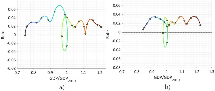
Figures 6–8 present GDP phase shadows for the six G7 countries.
Figure 6 shows the similarity in the behavior of the GDPN indicator for Canada and the United States,
when growth and slowdown are close in scale and time.
Figure 7 shows that for the United Kingdom, with the similarity of the behavior of the GDPN indicator
with France, there is a greater increase in the values of this indicator over the entire period of time. This is
not so clearly visible on the graphs of the plain GDPN time dependence for these two countries.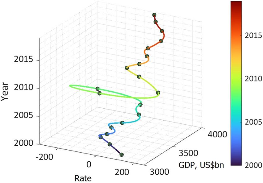
Applying spline-based phase analysis to macroeconomic dynamics 211 Figure 3: The German GDP phase shadow based on the spline approximation of statistical data over 2000–2019. Figure 4: Graphs of natural cubic splines interpolating the normalized GDP indicator for the G7 countries. Figure 5: GDP phase shadow for the German normalized GDP.
212 Gadasina Lyudmila and Vyunenko Lyudmila Figure 6: GDP phase shadows for Canada (a) and the United States (b). Figure 7: GDP phase shadows for the United Kingdom (a) and France (b). Figure 8: GDP phase shadows for Italy (a) and the Japan (b).

Applying spline-based phase analysis to macroeconomic dynamics 213
Figure 9: Phase shadow for German GDP 2000–2019: current prices (US$ billion).
In Figure 8, we can witness the complex dynamics of the GDPN indicator for Japan and Italy. At the same
time, the GDPN phase shadow for Italy shows a negative dynamics of the indicator, since a significant part of
the portrait is located in the negative range of rate values.
Important notes.
(1) When constructing phase shadow, it is important to choose model smoothing function that has the
minimal curvature on the considered time period. From this point of view, the use of, for example,
interpolation polynomials turns out to be incorrect, since it can induce false loops in phase shadows
and lead to an incorrect economic interpretation. Spline is considerably “stiffer” than a polynomial in
the sense that it has less tendency to oscillate between data points.
(2) When conducting an economic analysis, it is important to consider data in constant prices. Phase
shadows allow us to clearly identify the problem associated with the use of indicators at current prices.
Figure 9 shows a phase shadow of German GDP based on data measured in current prices. This figure
shows additional false loops that do not have a reasonable economic interpretation, whereas in Figure
3, there are no such dummy loops.
(3) When comparing the dynamics of indicators for different objects (in our case, the G7 countries), it is
necessary to normalize the initial data. In our empirical study, we normalized the GDP indicator for 2010.
4 Discussion
Empirical analysis has shown that phase shadows are an appropriate tool for studying the dynamics of
macroeconomic indicators. Herewith, interpolating by natural cubic splines is well suited for smoothing
low-frequency aggregated data.
When applying the approach outlined in the article, it is necessary to take into account the peculiarities
of calculating the analyzed indicators. It is important to consider the data in constant prices, and at the
same time, when comparing phase shadows for different subjects, it is necessary to normalize the
indicators.
The results clearly illustrate the events in the global economy. Applying the proposed method for a set
of indicators study allows identifying crises and examining their phases, both a posteriori, and forward by
making forecasts based on spline extrapolation of data. The outlined approach has a good development
prospect for frequent data as well.
Funding information: This research was funded by the project Russian Foundation for Basic Research
(RFBR). Project number: 20-010-00960.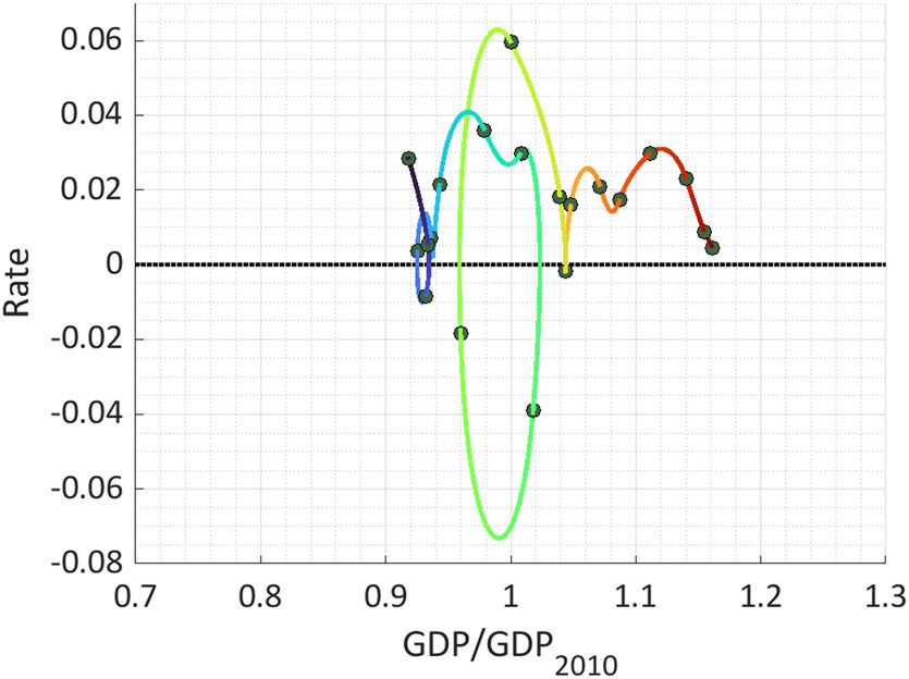
214 Gadasina Lyudmila and Vyunenko Lyudmila
Conflict of interest: The authors state no conflict of interest.
References
[1] Bao, H. X., & Wan, A. T. (2004). On the use of spline smoothing in estimating hedonic housing price models: Empirical
evidence using Hong Kong data. Real Estate Economics, 32(3), 487–507.
[2] Chakroun, F., & Abid, F. (2014). A methodology to estimate the interest rate yield curve in illiquid market. The Tunisian
Case. Journal of Emerging Market Finance, 13(3), 305–333.
[3] Holladay, J. C. (1957). Smoothest curve approximation. Mathematical Tables and Other Aids to Computation, 11(60),
233–243.
[4] Ilyasov, R. K. (2022). Flows in the digital economy: New approaches to modeling, analysis and management. In:
P. V. Trifonov & M. V. Charaeva (Eds.), Strategies and trends in organizational and project management. (DITEM 2021
(Lecture Notes in Networks and Systems, vol. 380). Cham: Springer.
[5] Leng, N., & Li, J.-C. (2020). Forecasting the crude oil prices based on Econophysics and Bayesian approach. Physica A:
Statistical Mechanics and its Applications, 554, 124663.
[6] Machado, J. A. T., & Mata, M. E. (2015). Pseudo Phase Plane and Fractional Calculus modeling of western global economic
downturn. Communications in Nonlinear Science and Numerical Simulation, 22(1–3), 396–406.
[7] Roul, P., & PrasadGoura, V. M. K. (2022). An efficient numerical method based on redefined cubic B-spline basis functions
for pricing Asian options. Journal of Computational and Applied Mathematics, 401, 113774.
[8] Takens, F. (1981). Detecting strange attractors in turbulence. Dynamical systems and turbulence, lecture notes in
mathematics, (Vol. 898, pp. 366–381). Berlin, Heidelberg: Springer.
[9] Tarasov, V. E. (2020). Fractional econophysics: Market price dynamics with memory effects. Physica A: Statistical
Mechanics and its Applications, 557, 124865.
[10] Vorontsovskiy, A. V., & Vyunenko, L. F. (2014). Constructing of economic development trajectories by approximating
conditions of stochastic models of economic growth. St Petersburg University Journal of Economic Studies, 37(3), 123–147.
[11] Waelde, K. (2011). Production technologies in stochastic continuous time models. Journal of Economic Dynamics and
Control, 35, 616–622.
[12] World Bank DatabankWorld Development Indicators. https://databank.worldbank.org/source/world-development-
indicators# (accessed on 1 February 2022).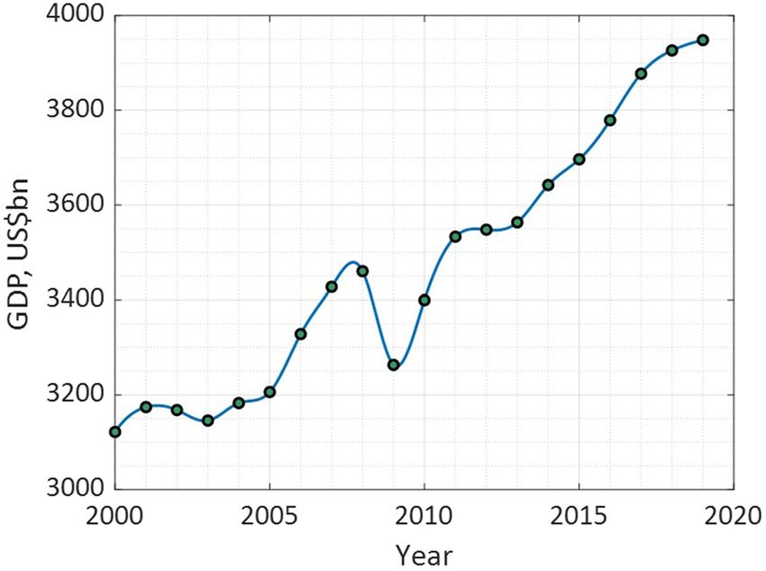
You can also read