Appendix A: Oregon Sea Otter Population Model, User Interface App
←
→
Page content transcription
If your browser does not render page correctly, please read the page content below
Appendix A: Oregon Sea Otter Population Model, User Interface App
                                   (“ORSO” v 1.0)

Dr. M. Tim Tinker
Research Biologist, Nhydra Ecological Consulting, Head of St. Margaret’s Bay, NS
Adjunct Professor, Department of Ecology and Evolutionary Biology, University of California Santa Cruz
Contents
1      Introduction/Context ........................................................................................................................... 1
2      Methods ............................................................................................................................................... 1
    2.1        Overview ...................................................................................................................................... 1
    2.2        Demographic processes ............................................................................................................... 2
    2.3        Spatial Processes .......................................................................................................................... 3
    2.4        Estimating K and Habitat Effects .................................................................................................. 6
    2.5        Establishment Phase .................................................................................................................... 6
    2.6        Model Simulations ....................................................................................................................... 8
3      Simulation Results: Sample Scenario ................................................................................................. 10
Oregon Sea Otter Population Model (ORSO), User Interface .................................................................... 14
    Overview ................................................................................................................................................ 14
    Components of ORSO App ..................................................................................................................... 15
       Setup Model Simulations Panel ......................................................................................................... 15
References ................................................................................................................................................. 25

                                                                               i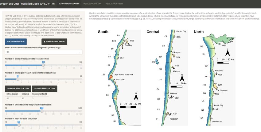
1     Introduction/Context
The Oregon sea otter population model has been developed as a user-friendly interface for community
members and managers to explore possible sea otter recovery patterns after introduction. The model
can contribute to responsible stewardship of sea otters and other nearshore marine resources. The
overall goal of the Oregon sea otter population model is to anticipate the approximate magnitude of
expected population growth and spread of sea otters in coastal Oregon in the foreseeable future, under
different scenarios of translocation/re-introduction. This information will help in evaluating
management options and anticipating ecological and socio-economic impacts in a spatially and
temporally explicit way. However, experience from prior reintroductions demonstrate that it is
extremely difficult to predict where translocated animals will settle, how many will remain following
release and how soon population growth will commence. This model is therefore not intended to
predict specific outcomes, but rather to explore a range of outcomes that may be most likely, given an
extensive range of model inputs and assumptions.

2     Methods
2.1    Overview
The model has been developed using information from published reports and previous examples of sea
otter introductions, population recovery and range expansion in the northeast Pacific. In particular, data
collected from areas of sea otter recovery in California, Washington and SE Alaska can be used to inform
our expectations for sea otter colonization and recovery in Oregon. The distinct habitats and differing
historical contexts of these neighboring populations preclude a direct translation of expected dynamics;
however, the data from studies of these populations can be used as the basis for developing a predictive
model that is tailored to the habitat configuration of Oregon.

Spatially structured population models have been constructed for other sea otter populations in North
America and have proved effective at predicting patterns of population recovery and range expansion in
diverse habitats (Udevitz et al. 1996, Monson et al. 2000a, Tinker et al. 2008, USFWS 2013, Tinker 2015,
Tinker et al. 2019a, Tinker et al. 2021). By building on these previously published model designs and
incorporating locally relevant data on sea otter vital rates, movements, habitat quality and
environmental parameters, it should be possible to define realistic boundaries for the expected patterns
of population abundance and distributional changes over time. These patterns can then be used as a
basis for designing an appropriate monitoring design for sea otters and the habitats they are expected
to affect, as change occurs over time. Such a model can also be used to combine and integrate
information on habitat impacts and sea otter monitoring data over time, allowing us to update
projections and modify monitoring methods; in essence, a quantitative tool for conducting adaptive
management.

Using data from comparable sea otter populations and geographic areas, primarily California (but also
augmented by data and models from SE Alaska and Washington), we developed a spatially explicit,
simulation-based population model for use in evaluating a range of realistic scenarios of sea otter re-
introduction to Oregon. The Oregon Sea Otter Model (ORSO) incorporates demographic structure (age
and sex), density-dependent variation in vital rates, habitat-based variation in population growth
potential, dispersal and immigration, and uses a spatial diffusion approach to model range expansion
over time.

                                                    1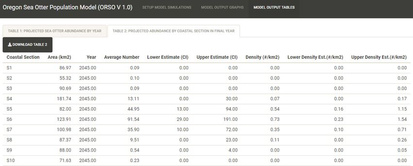
2.2   Demographic processes
As with previous sea otter models (Tinker 2015), the core of ORSO is a stage-structured projection
matrix describing demographic transitions and thus population growth over time (Caswell 2001). The
projection matrix is used to model transitions among four age/sex classes (c = 1:4): 1) juvenile females
(weaning-3 y), 2) adult females (3-20 y), 3) juvenile males
(weaning-3 y) and 4) adult males (3-20 y). Transition
probabilities are described by 3 parameters: stage-
specific annual survival (S), adult female reproductive
output (R, defined as the probability an adult female
gives birth to and successfully weans a male or female
pup into the juvenile age class), and the growth
transition parameter (G, the probability that juveniles
advance to the adult age class, conditional upon
survival). These demographic transitions can be
visualized as a loop diagram (Figure 1). Survival rates are
age- and sex-dependent and are assumed to vary
stochastically and as a function of population density
(Siniff and Ralls 1991, Eberhardt and Schneider 1994,       Figure 1 Loop Diagram of demographic transitions
Monson et al. 2000b, Tinker et al. 2006).                   for sea otters in population model

Reproductive contributions to juvenile stages by adult females are assumed to reflect a 50:50 sex ratio
at birth, and estimated as:

                                                    R f / m = Sa , f × 1 2 b × w                                        (1)

where b is birth rate (held constant at 0.98; Tinker et al 2006) and w is weaning success rate, which is
stochastic and density-dependent (Monson et al. 2000b). Note that equation 1 also reflects the fact that
pup survival is conditional upon adult female survival. Growth transitions for each sex are calculated
using the standard equation for fixed-duration age classes (Caswell 2001):

                                                   æ ( S j , f /m l )T - ( S j , f /m l )T -1 ö
                                          G f /m = ç                                          ÷                         (2)
                                                   è             ( S j , f /m l )T - 1        ø
where T is the stage duration for juveniles (2.5 years) and l is the annual rate of population growth
associated with a specified matrix parameterization. Combining all parameters into matrix form, we
estimate annual population dynamics using matrix multiplication (Caswell 2001):

                        æ n1,t +1 ö æ (1 - G f ) S j , f      Rf                 0                 0 ö æ n1,t ö
                        ç         ÷ ç                                                                    ÷ ç ÷
                        ç n2,t +1 ÷ = ç G f × S j , f        Sa , f             0                  0 ÷ ç n2,t ÷         (3)
                        ç n3,t +1 ÷ ç                                                                    ÷´
                                            0                Rm           (1 - Gm ) S j ,m         0 ÷ ç n3,t ÷
                        çç        ÷÷ ç                                                                      ç ÷
                           n
                         è 4,t +1 ø è ç     0                 0             Gm × S j ,m           Sa ,m ÷ø çè n4,t ÷ø

In equation 3, the population vector nc,t tracks the abundance of otters in each age/sex class in year t of
a model simulation. At low population abundance (defined as S nc,t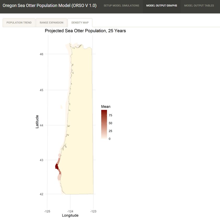
Parameterization of vital rates was based on published data for sea otter populations in California,
Alaska and Washington (Siniff and Ralls 1991, Monson and Degange 1995, Garshelis 1997, Gerber et al.
2004, Tinker et al. 2006, Laidre et al. 2009, Tinker et al. 2017, Tinker et al. 2021). Results from past work
suggests that much of the variation in age specific survival and weaning success is explained by density
with respect to carrying capacity, although individual variation and random year-to-year variation (i.e.
environmental stochasticity) can also be important (Staedler 2011, Miller et al. 2020). Accordingly,
following methods used in other simulation models (Gerber et al. 2004, Bodkin and Ballachey 2010), we
sampled from the survivorship schedules reported for populations at varying densities (ranging from
low-density, rapidly growing populations to high density populations at carrying capacity) to inform our
model. We collapsed all age-structured data down to the age/sex classes using geometric averaging of
the annual rates for year-classes in each age class, and we accounted for uncertainty by drawing from
beta distributions with means and variances corresponding to the published data sets. Re-sampling
from these distributions we created a table of 1000 sets of vital rates (survival, birth rates and weaning
success rates) reflecting the full range of potential demographic schedules for sea otter populations
having biologically feasible growth rates (0.90
efficiency, continuous diffusion dynamics can be approximated within a discretized matrix model by
incorporating key features and predictions (e.g. the asymptotic invasion speed of the frontal edge of a
population). Discretization can be especially effective if the population is divided into relatively small
sub-sections such that demographic processes vary between sub-sections but can be assumed to be
approximately homogeneous within sections.

In the case of ORSO, because range expansion was one of the key features we wished to address, we
divided the region of interest (all coastal areas of Oregon) into 42 coastal sections, each spanning
approximately 15 km of the outer coastline and/or encompassing a single coastal estuary (Figure 2).
Annual intrinsic dynamics (changes in abundance due to births and deaths) are modeled for each coastal
section using equations 3 and 4; however, each of these sub-populations is embedded within a range-
wide meta-population that allows for dispersal of animals between occupied sections. Range expansion
of the meta-population along the coast is incorporated into the model by allowing un-occupied sections
to be “colonized” by animals from neighboring occupied sections, with the rate of colonization of new
sections constrained to maintain a pre-specified rate of advance of the population front along the coast
(henceforth n, the asymptotic frontal wave speed, measured in km/year; Figure 3). We treat n as a user-
specified parameter, noting that a realistic range of values based on previous studies is 1–5 km/year
(Lubina and Levin 1988, Tinker et al. 2008).

Figure 2. Spatial configuration of coastal habitat in Oregon used for population model. Coastal habitat sections (labeled
polygons) show the basic geographic unit for modeling demographic processes, while the colored spatial grid within these
olygons show the relative expected density at carryign capcity, based on a previously-developed model of habitat-density
relationships (Tinker et al. 2021, Kone et al., in press).

                                                               4
Dispersal of sea otters between coastal sections is
modeled and tracked separately for each age/sex
class in ORSO, reflecting the different mobility and
dispersal capability of sea otters of different ages
and sex (Jameson 1989, Tarjan and Tinker 2016,
Breed et al. 2017). We used previously collected
data from radio-tagged sea otters to estimate
probabilities that otters of each age/sex class
emigrate from coastal section i to coastal section j in
a given year. To account for occasional (but
Figure 3. Schematic drawing illustrating how model
potentially important) long-distance dispersal, we
incorporates range expansion of sea otter population from
do not restrict dispersal to adjacent cells only: occupied habitat into un-occupied habitat
rather, we used the empirical distribution of annual
dispersal distances to parameterize this step. For
each tagged animal and each year of monitoring we computed “NLD”, the net annual linear
displacement (Tarjan and Tinker 2016), defined as the number of kilometers between an animal’s
location at the start of the year and its location at the end of the year in terms of the swimmable
distance along the coast1. We used maximum likelihood methods to fit exponential distributions to NLD
data collected from otters of each age/sex class (implemented using the “fitdistr” library in R). We then
used the fitted exponential distributions to calculate the cumulative distribution function (CDF) values at
zi, defined as the average distance from the centroid to the boundary of each coastal section i: these
computed CDF values correspond to the mean probability of remaining within coastal section i for an
otter of a specified age/sex class (Tinker et al. 2008), the inverse of which represents dc,i, the per-capita
probability of emigration from section i for an otter of class c.
The actual number of otters of class c emigrating from section i in year t (dc,i,t) was randomly drawn from
a Poisson distribution with rate parameter nc,i,t ·dc,i. To determine where emigrating otters dispersed to,
we first computed the swimmable distances between all pairwise combinations of section centroids, and
for each pairwise distance (Di,j) we used the fitted exponential functions to calculate the probability
density function (PDF) values at x = Di,j. Then during each year of a model simulation we identified the
set of all other currently-occupied sections (j = 1,2… J, j ¹ i), re-scaled the PDF values such that
SPDFi,j = 1, and then drew randomly from a multinomial distribution with probability parameters PDFi,j
to determine which coastal section j would “receive” the emigrating otters. In this way, emigration was
treated probabilistically and not deterministically, so that each iteration of the simulation model results
in different dispersal outcomes. We note that spatial processes (dispersal and range expansion) are
expected to differ during the post-introduction establishment phase, and thus we allow for modified
spatial dynamics during this period, as described below (section 2.5).
1
The distinction of swimmable distance is important: we used swimmable distances as opposed to Euclidean
distances because of the complex coastal topography of sea otter habitats and the fact that sea otters cannot
travel over land. This for the purpose of calculating NLD, and for all other distance calculations described in the
methods, we used a Least Cost Paths function (implemented using the “gdistance” package in R) which estimates
the shortest distance between two points while accounting for the “costs” of moving through different habitat
classes that might be encountered between the points. By assigning a prohibitively high “cost” to moving over
land, we ensure that the Least Coast Path distance is the shortest distance through water only.
52.4 Estimating K and Habitat Effects
Carrying capacity (K) is defined as the population size that can be supported in a specified environment
over the long term, and this equilibrium abundance is generally dictated by some limiting resource (i.e.
prey, nesting sites, refuge habitat). In sea otters, K is thought to be primarily determined by prey
resource abundance and productivity. Equilibrium abundances of sea otter populations have been
found to be highly variable, with local densities ranging from 0.5 sea otters per km2 of benthic habitat
(defined as benthic substrate between the low tide line and the 40 m depth contour) to over 20 sea
otters per km2. Previous studies have found that the density at K varies as a function of certain habitat
features (presumably because these habitat features are proxies for prey productivity), however the
precise nature of these relationships varies across regions (e.g. Laidre et al. 2001, Laidre et al. 2002,
Burn et al. 2003, Gregr et al. 2008, Tinker et al. 2021). In California, areas of rocky substrate were found
to support higher densities than areas of unconsolidated sediment (Laidre et al. 2001), while in
Vancouver Island it was areas of complex coastline that supported higher densities (Gregr et al. 2008),
and in SE Alaska some of the highest densities are supported in soft-sediment bays (Esslinger and Bodkin
2009). Given this variation, it is difficult to predict which habitat types in Oregon will eventually support
high or low densities of sea otters. However, given the proximity to California and the general similarity
of habitat types between these regions, we believed that California habitat-density relationships provide
the best starting point for predicting these relationships in Oregon. A recently developed model
predicting local carrying capacity as a function of biotic and abiotic habitat variables (Tinker et al. 2021)
has therefore been applied to the equivalent spatial layers of habitat variables in Oregon, in order to
project potential carrying capacity at fine scales throughout the state (Kone et al. in press). We use this
projected carrying capacity data layer to parameterize the ORSO model, interpolating projected
equilibrium densities from Kone et al. (in press) at each cell h of a hexagonal grid laid over the study area
(Figure 2). The absolute number of otters expected within grid cell h at carrying capacity is calculated as
the product of the expected equilibrium density (Khd) and the area of that cell (Ah). Summing this
product over all habitat cells contained within coastal section i (h = 1, 2,…Hi) gives the expected
abundance at K for that section (used for equation 4), and dividing by Ai (the total area of habitat in
section i) gives the mean expected density at K for coastal section i:
Hi
1
K =
i
d
Ai
åK
h =1
d
h × Ah (5)
2.5 Establishment Phase
Previous translocations and re-introductions of sea otters have shown that the years immediately after
re-introduction can be a period of great uncertainty (Jameson et al. 1982, Bodkin et al. 1999, Carswell
2008, Bodkin 2015). During this population establishment phase there is limited population growth and
often a significant decline in abundance, associated with elevated mortality and dispersal of a
substantial proportion of animals away from the release site. Otters that disperse from the introduction
site may settle at other areas of suitable habitat within the region (as occurred in SE Alaska), return to
their former home ranges if possible (as occurred at San Nicolas Island), or move entirely out of the
region (as was suspected to have occurred for some animals in the Oregon translocation, believed to
have moved north to join the Washington or BC populations), though in all cases there is likely to be
significant mortality for both dispersing and non-dispersing animals. Thus, the “typical” patterns of
density-dependent population growth, dispersal, and range expansion, described in the previous
6sections, only emerge after this establishment phase, which may extend for 5-20 years after the initial
translocation (Jameson et al. 1982, Bodkin et al. 1999, Carswell 2008, Bodkin 2015).
To model establishment phase dynamics, we define several additional parameters and associated
functions. The first of these is E, the expected duration of the establishment phase itself (in units of
years). For all years where t £ E, we adjust the baseline age and sex specific survival rates (Sc,t, the
random survival rates selected based on the solution to equation 4) such that the mean growth rate (l)
is forced to 1 (i.e., no net growth on average) but with default levels of environmental stochasticity. We
next define parameter M, the mean excess annual mortality rate during the establishment phase: this
parameter, assumed to occur within the range of 0 < M < 0.5, is used to further adjust stage-specific
annual survival rates during the establishment phase, thereby allowing for negative growth rates:
Sc' ,t = Sc,t × (1 - mt ) , where mt ~ Beta (a , b | M ) (6)
In equation (6), the annual excess mortality rate (mt) is drawn from a Beta distribution with parameters
a and b, which are set so as to create a 0 – 1 bounded distribution with mean of M and coefficient of
variance (CV) of 0.25, a level of variation consistent with previously published demographic schedules
(Gerber et al. 2004, Tinker et al. 2019b). The modified stochastic survival rates (S’c,t) are used to
parameterize the population projection matrix P (equations 1-3 above) for each year during the
establishment phase. Thus, if we define the initial population vector of introduced animals as nc,0 (where
N0 =S nc,0), then the survivors in year 1 are calculated via matrix multiplication as nc,1 = P0 * nc,0.
For those otters that survive the initial re-introduction, we assume that a substantial number will
disperse a significant distance away from the re-introduction site. We define j as the expected
probability of dispersal away from the reintroduction site during the establishment phase (0 < j < 1),
and calculate the actual number of dispersers (D*) as a random binomial variable:
D* ~ Binomial ( N1 , j ) (7)
where N1 is the number of individuals that survived the initial translocation. The stage structure of the
disperses is assigned randomly using a multinomial distribution with probabilities corresponding to the
stage structure of nc,1. Several lines of evidence suggest that the probability of post-introduction
dispersal (j) may be affected by one or more covariates, including the age structure of the introduced
population and the release site habitat. Specifically, in the case of the San Nicolas translocation it was
observed that younger animals (sub-adults) were more likely to remain at the release sites than adults,
with the latter more likely to attempt to return to their original home ranges (Carswell 2008). It has also
been suggested that otters introduced into estuarine habitats may be more likely to remain resident
(Hughes et al. 2019, Becker et al. 2020), and this may be especially true if enclosures are set up to retain
some animals until they become familiar with estuarine prey and substrates. We therefore included two
additional parameters to account for these potential covariates: we define w as the expected ratio of
dispersal probability for subadults relative to adults (0 < w < 1), and y as the expected ratio of dispersal
probability for otters in estuaries relative to outer coast habitats (0 < y < 1). If we define j as the
probability of dispersal for a group of adults in an outer-coast environment, then the realized dispersal
probability for a given section (ji’) is calculated as:
ji ' = j × ( RAd ,i + w × (1 - RAd ,i ) ) × ( (1 - Esti ) +y × ( Esti ) ) (8)
7where RAd,i is the ratio of adults to sub-adults introduced to section i, and Esti is a switch variable that
indicates whether section i is an estuary (Esti = 1) or outer coast (Esti = 0).
To allow for the likelihood that a significant proportion of the animals dispersing from the reintroduction
site will either die or else move outside of the study region (i.e., outside of coastal Oregon, possibly
joining the Washington or California populations), we define parameter W as the loss rate for dispersing
animals. The remaining dispersers, calculated as D*(1-W), are assumed to settle in one of the other
coastal sections (Figure 2), which is selected randomly from a multinomial distribution with parameters
proportional to the mean K densities of each section (equation 5), thereby assuming that the dispersers
are more likely to settle in an area of higher quality habitat.
All of the above-described parameters may be adjusted by the user to explore assumptions about the
establishment phase and its implications for success of a proposed re-introduction. We note that the
setting parameters to values close to their defaults (E = 10, M = 0.15, j = 0.9, w = 0.5, y = 0.5, W = 0.7)
will produce dynamics (on average) that match the observed population dynamics at San Nicolas Island
during the 3 decades after that translocation.
2.6 Model Simulations
Having developed and parameterized ORSO as described in the previous sections, we use this model to
conduct simulations of sea otter population dynamics in Oregon for a newly established population.
Simulations are run to evaluate population growth and range expansion under different re-introduction
scenarios and under varying sets of assumptions about population dynamics, as reflected by different
combinations of user-specified parameters (see Table 1 for complete list of user-specified parameters,
definitions, and suggested values). A stepwise description of model parameterization and dynamics
(“pseudo-code”) is as follows:
1. Select coastal sections for re-introducing sea otters and specify the numbers of animals (N0,i) to
be introduced to each section, both during the initial year of translocation, and optionally as
“supplemental” additions of more otters in subsequent years (Oi,t). The age/sex composition of
introduced otters is also specified: RAd,i is the ratio of adults to subadults, and RF,i is the ratio of
females to males.
2. User adjusts the expected values of other parameters to investigate their effects: parameters
that can be adjusted include maximum population growth rate (rmax), environmental
stochasticity in growth rates (s), the functional shape of density-dependence (q), asymptotic
wave speed for population range expansion (n), the number of years required for the population
to become established (E), the excess annual mortality rate during establishment phase (M), the
probability of dispersal for adults post-introduction (j), the dispersal probability adjustment for
subadults relative to adults (w), the dispersal probability adjustment for otters in estuaries (y)
and the proportion of dispersers lost (W).
3. Iterate a large number of simulations (“reps”), each one describing “Nyrs” years of population
dynamics (both reps and Nyrs are user-adjustable, default = 100 reps of 25 years)
4. Step through the processes of population dynamics for t = 1, 2,…Nyrs. For each year of each
simulation, the model conducts the following steps:
a. During establishment phase (t £ E), calculate proportion of animals that disperse away from
release site (accounting for age and estuary effects), stochastically chose a target coastal
8section for these dispersers, and move the dispersers to that location accounting for losses
due to death and emigration out of coastal Oregon.
b. If establishment phase complete (t > E), determine any new sections that have become
occupied since the previous time step: a section is eligible to be colonized depending on its
distance to a neighboring occupied section, the number of years the neighboring section has
been occupied, and the value of n, as illustrated in Figure 3.
c. For all sections occupied at time t, calculate intrinsic population growth rates (equation 4).
Draw random sets of vital rates corresponding to li,t and use these to parameterize
projection matrix Pi,t following equation 3. If establishment phase (t £ E), adjust rates
accordingly based on parameter M (equation 6). To account for spatial autocorrelation in
environmental stochasticity, values of ei,t are drawn from a multivariate normal distribution
with mean of 0 and co-variance matrix adjusted (using standard auto-regressive methods)
to produce standard deviation s and correlation across neighboring sections of 0.8 (Gelfand
and Vounatsou 2003).
d. If establishment phase complete (t > E), draw randomly from Poisson distribution (with rate
parameters nc,i,t ·dc,i) to determine how many (if any) otters of each age/sex class disperse
from section i (dc,i,t).
e. Draw randomly from multinomial distribution (with probability vector PDFi,j) to determine
which occupied sections will receive the dispersers from section i.
f. Calculate the stage-specific change in abundance for section i in year t as:
nc,i ,t = Pi ,t × nc,i ,t -1 - dc,i ,t + å ac, j ,i ,t + oc,i ,t (9)
j
where dc,i,t represents dispersal of animals out of section i in year t, ac,j,i,t represents otters
dispersing into section i from any other occupied section j in year t, and oc,i,t represents
additional supplemental otters introduced to section i (the numbers of these supplemental
otters, age/sex, and number of years that otters are added are all adjustable parameters).
5. Tabulate the abundance of otters in each section for each year of each model simulation.
6. Down-scale estimated densities to the scale of 1-km2 habitat cells by spatial-interpolation
between section centroids, weighted by the habitat suitability index of each cell (equation 5).
7. Summarize results graphically and in tables.
The complete R code used to run ORSO is provided in Appendix A, and digital versions of this code as
well as the associated data files needed to run it are available upon request.
The user-specified parameters can be varied independently to produce an enormous range of different
dynamics, allowing users to create and explore highly customized scenarios. For illustrative purposes we
present results for a “typical” scenario, using values provided in Table 1.
9Table 1. Default values for user-specified parameters for Haida Gwaii Sea Otter Recovery Habitat Model (HGSORHM).
User Param Default Value Explanation
reps 100 Number of replications for population simulations
Nyrs 25 Number of years to project population dynamics
Intro_Sections NA Coastal section(s) for re-introduction
N0,i 50 Number of otters introduced to each specified coastal section
Oi 3 Number otters (annually) in supplemental introductions to section i
Nyrs_add 5 Number of years for supplementary introductions
RF,i .6 Proportion of introduced animals that are female
RAd,i .25 Proportion of introduced animals that are adult
E 10 Expected years before population becomes fully "established" (i.e. before
“normal” population growth and range expansion begins)
M .15 Mean excess annual mortality rate during the establishment phase
j .7 Probability of dispersal (for adults) in establishment phase
w .5 Dispersal probability adjustment for subadults relative to adults
y .5 Dispersal probability adjustment for otters in estuaries
W .75 Proportion of post-introduction dispersers lost (die or move out of study area)
n 2 Asymptotic wave speed of range expansion, km/yr, minimum
rmax 0.18 Maximum instantaneous rate of growth: default rmax=0.2 (Note: exp(0.2) =
1.22 or 22% per year)
s 0.1 Environmental stochasticity (std. deviation in log-lambda)
q 0.9 theta parameter for theta-logistic model: for standard Ricker model, theta = 1;
for delayed onset of D-D effects, use theta > 1
3 Simulation Results: Sample Scenario
The ORSO model simulations can produce a broad range of projected patterns of growth and range
expansion, appropriately reflecting the large amount of uncertainty about the future after a re-
introduction event. The outcome after 25 years (in terms of the magnitude of growth and
extent/pattern of range spread) depends upon the re-introduction scenario and the various assumptions
implicit in the user-specified parameters (Table 1). For areas of Oregon that do become occupied, the
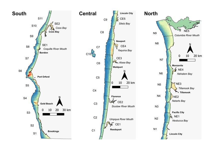
model predicts fine-scale spatial variation in sea otter densities after 25 years, explained in part by the
length of time a particular area is occupied, and in part by the suitability of the local habitat (Figure 2).
Running model simulations with “typical” values for user-specified parameters (Table 1) revealed that
that an initial translocation of 50 otters to coastal section S6 (assuming 60% female and 25% adult), with
supplemental additions of 3 juveniles per year for 5 years, could grow to a population of approximately
78 sea otters after 25 years (Figure 5), although there is considerable uncertainty around this value (CI95
= 17 - 190). Range expansion over this period is projected to be limited to the southern portion of
Oregon coast (coastal sections S1-S11; Figures 5, 6). This fairly low rate of growth and range spread
reflects a population establishment phase of 10 years as well as a relatively low diffusion rate (n = 2
km/year), which is comparable to the rate of range spread observed for California and Washington state
(Tinker et al. 2008, Laidre et al. 2009). We note that changing the user-specified parameters can lead to
considerably different projections of both population growth and range expansion.
10Figure 4. Map of coastal Oregon showing projected sea otter abundance and distribution after 25 years.
11Figure 5. Results from model simulations of sea otter population dynamics over 25 years in coastal Oregon, showing
projected population trends. Light gray band shows 95% CI for simulations; dark gray band shows 95% CI for mean.
12Figure 6. Results from model simulations of sea otter population dynamics in coastal Oregon, showing a heatmap of
mean expected abundance by Coastal Section over a 25-year period. Refer to figure 2 for locations and boundaries of
each coastal section.
13Oregon Sea Otter Population Model (ORSO), User Interface
https://nhydra.shinyapps.io/ORSO_app/
Overview
The web based ORSO app is organized into several panels, which the user can navigate between by
clicking on any of the three selection tabs embedded in the title bar at the top of the screen, as shown in
the Figure below (items A, B and C). The panel that is active by default when the app is opened is
“SETUP MODEL SIMULATIONS”, while the other two panels (“MODEL OUTPUT GRAPHS” and “MODEL
OUTPUT TABLES”) can be navigated to by the user to view model results AFTER having run simulations.
When active, the “SETUP MODEL SIMULATIONS” panel is itself divided into two main sections: a sidebar
panel at left (item D) where the user can adjust various parameters and run the simulations; and an
information panel at right (item E), which shows a map of Oregon with coastal sea otter habitat (the
nearshore zone out to 60 m of depth, plus estuaries) divided into 42 numbered coastal sections. These
coastal sections represent the main spatial units for tracking sea otter abundance and distribution over
time: the map allows the user to see the location of specific sections, as needed to initiate simulations
and interpret model results.
A B C
D
E
14Components of ORSO App
Setup Model Simulations Panel
At the top left of the sidebar panel are some simple instructions to guide the user, and two large
buttons: “Run Simulations Now” and “Download User Manual”.
The “Download User Manual” button at right allows the user to download this manual at any time. The
“Run Simulations Now” button at left is the primary action button of ORSO, used to run a set of
simulations. HOWEVER, this button should only be clicked AFTER having first selected one or more
coastal sections under consideration for a sea otter re-introduction and setting the user-adjustable
parameters in the sidebar panel that describe the details of the reintroduction and control the
underlying assumptions about the nature of population growth and range expansion. A description of
each of the user-adjustable parameters will appear when the cursor is moved over top of the name of
each parameter, and default values for each parameter are set based on data from other sea otter
populations. These user-parameter adjustment controls are illustrated and explained below:
Select coastal sections for reintroduction and numbers of otters to be added
Clicking on the selection box at top reveals a drop-down list of the 42 coastal sections (whose
geographic locations can be viewed on the map at right), from which the user can select a coastal
section where sea otters are to be introduced. Next, the two sliders below the selection box can be
used to adjust the number of otters in the initial translocation event, as well as (optionally) the annual
number of animals added to this section as part of supplementary introductions in subsequent years.
15Clicking on the “Update Introduction Table” button will add these user selections to a parameter table
below the button. The user can then repeat this process (if desired) to specify additional coastal
sections and associated translocation parameters and add those to the parameter table. To clear the
table and start again at any time, click on the “Clear Introduction Table” button.
Adjust number of iterations
This slider control is used to increase or decrease the number of simulation iterations: that is, the
number of times a population simulation is replicated with random draws of all appropriate stochastic
parameters. Increasing the number of replications of a simulation improves the precision of model
predictions but will take longer to run. At least 100 iterations are suggested.
Adjust number of years
This slider control is used to increase or decrease the number of years into the future the simulation is
run. Increasing the number of years ('N') can provide insights into conditions farther in the future, but
results become less reliable the farther ahead in time the model is projected.
Adjust number of years that supplemental introductions occur
This slider control is used to increase or decrease the number of years after the initial translocation
event in which additional otters may be added to the initial reintroduction site (supplemental
reintroductions). Adding more otters could potentially improve success of the reintroduction by
stabilizing the population during the establishment phase. These additional otters could be wild otters
or juvenile re-habilitated otters from captivity.
Adjust sex ratio of reintroduced otters
This slider control allows the user to specify the proportion of introduced otters that are female.
Including a higher proportion of females can increase the potential for growth, though there must be at
least some adult males for reproduction to occur.
16Adjust age composition of reintroduced otters
This slider control allows the user to specify the proportion of introduced otters that are adult (vs sub-
adult or juvenile). Only adult sea otters produce pups, so introducing adults can hasten reproduction.
However, in past translocations it has been found that sub-adults may be more likely to successfully
'take' to their new habitat, so a higher ratio of sub-adults may improve success.
Adjust duration of “population establishment” phase
Newly established sea otter populations often experience an initial period of reduced growth and
limited range expansion, as the population becomes established. This establishment period has varied
from 5-15 years in previous re-introductions and natural return events. This slider control allows the
user to set the expected duration of this phase. In addition to reduced survival rates and range
expansion during the establishment period, the user can specify the probability of post-introduction
dispersal away from the release site.
Adjust excess mortality during establishment
During the establishment phase of an introduced population, there may be higher than average levels of
mortality as the introduced animals become accustomed to their new habitat. In past translocations,
excess annual mortality rates of 0.1 - 0.25 have caused translocated populations to decline substantially
during the establishment phase
Adjust probability of dispersal during establishment phase (adults)
In several previous sea otter translocations, a substantial proportion of the introduced animals moved a
significant distance away from the introduction site during the establishment phase. The details and
destination of post-release dispersal is impossible to predict, but the user can set the mean expected
proportion of otters to disperse.
17Adjust probability of dispersal during establishment phase for subadults
In previous sea otter translocations, it has been observed that subadult animals may be less likely to
disperse than adults (i.e. more likely to remain near the introduction site). This parameter adjusts the
likelihood of dispersal for subadults as compared to adults: a value of 0.25 would mean that subadults
are 1/4 as likely to disperse as adults.
Adjust probability of dispersal during establishment phase for otters in estuaries
Based on several lines of evidence it has been suggested that otters re-introduced to estuaries may be
less likely to disperse (i.e. more likely to remain near release sites) than otters added to outer coast
habitats. This parameter adjusts the likelihood of dispersal for estuaries as compared to open coast: a
value of 0.25 means otters in estuaries are 1/4 as likely to disperse post-introduction.
Adjust mortality rate of otters that disperse during establishment phase
The fates of otters that disperse away from a re-introduction sites is hard to determine in most cases: in
some reintroductions there appears to have been high levels of mortality for dispersers, in others there
is emigration to a different region altogether. This parameter sets the expected loss-rate for the
dispersers: that is, the proportion that die or move entirely out of the study area (and are effectively lost
to the Oregon meta-population).
18Adjust rate of range expansion
This slider control allows the user to adjust the expected rate at which the growing population spreads
into new habitat. Distribution of the initial sea otter
population will likely be limited to a relatively small
area(s) of the coast where sea otters are introduced.
As the population grows it's distribution (range of
occupancy) will spread outwards along the coastline,
encompassing more habitat. The rate of range
expansion is measured as the speed at which the
frontal edge of the population moves along the
Schematic drawing illustrating how the model
coastline (Figure 3). In other populations, this range
incorporates range expansion of sea otter population
from occupied habitat into adjacent unoccupied habitat expansion speed has varied from 1 to 5 km/year.
Adjust maximum rate of growth
Sea otter populations tend to show the highest rate of growth at low densities: as local abundance
increases, the growth rate slows until it eventually reaches 0 when population abundance reaches
carrying capacity, or 'K'. This slider control allows the user to adjust the maximum rate of growth (at low
densities): in most sea otter populations this value is between 0.15 and 0.20.
Adjust environmental stochasticity
The average rate of growth for a re-establishing sea otter population in a given area can be predicted as
a function of the local density with respect to carrying capacity, or 'K'. However, year-to-year variation in
environmental conditions and prey population dynamics can lead to unpredictable deviations in growth
rate, referred to as 'environmental stochasticity'. This slider control can be used to adjust the degree of
annual variation in growth rates: typical values are 0.05 - 0.15.
19Adjust ‘theta’ parameter, for theta-logistic growth
The average rate of growth for a re-establishing sea otter population in a given area can be predicted as
a function of the local density with respect to carrying capacity, or 'K'. One of the parameters of this
function is 'theta', which determines the nature of the onset of reduced growth rates at higher
densities: 'theta' values 1 mean that significant reductions in growth occur only at higher densities. This slider control
can be used to adjust 'theta': typical values reported for marine mammals are between 0.8 and 2, and a
recent study in California reported a value of close to 0.9 for southern sea otters.
20MODEL OUTPUT GRAPHS Panel
After setting up and running simulations, the user can navigate to the “MODEL OUTPUT GRAPHS” panel
in order to view graphical results from model simulations. There are three separate graphs that can be
viewed, and the user can move between these by selecting one of the three graph selection tabs just
below the title bar.
Population Trend Graph
This plot shows the projected abundance over time of sea otters in Oregon, based on results from the
simulation model (EXAMPLE SHOWN IS FOR ILLUSTRATIVE PURPOSES ONLY). The horizontal axis
represents years into the future, while the vertical axis represents the expected total number of sea
otters in a given year. Uncertainty about model results is calculated based on the distribution of results
from stochastic iterations of the simulation. The solid black line represents the average abundance
trend (i.e. averaged across all iterations), the dark grey band shows the 95% CI for the mean trend (i.e.
uncertainty about the true average), and the light grey band shows the 95% CI for the full distribution of
results (i.e. uncertainty about the range of possible outcomes).
21Range Expansion Graph
This heatmap graph shows the average projected abundance and spatial distribution of sea otters over
time (EXAMPLE SHOWN IS FOR ILLUSTRATIVE PURPOSES ONLY). Each grid cell represents a coastal
section (vertical axis), as defined by the map on the front page, on a given year (horizontal axis): the
shading of the grid cells indicating the relative abundance of sea otters (darker colors = more otters,
white cells = no otters). The increase from left-to-right in the number and intensity of shaded cells
illustrates the spatiotemporal patterns of range expansion. At the left-hand side of the heatmap (year
1), the spatial distribution is constrained by the starting conditions (density = 0 at all but the section(s)
where sea otters are introduced). As one moves from left to right across the heatmap (i.e. moving
forward through time), the changes in density and distribution reflect the rates of population growth
and range expansion.
22Density Map
This map figure of coastal Oregon shows the average projected abundance and distribution of sea otters
at the end of the simulation period (EXAMPLE SHOWN IS FOR ILLUSTRATIVE PURPOSES ONLY). The
mean expected number of sea otters in each coastal section (for the specified reintroduction scenario) is
illustrated by the shading of the nearshore habitat zone, with darker shades of red-brown indicating
higher abundances of sea otters.
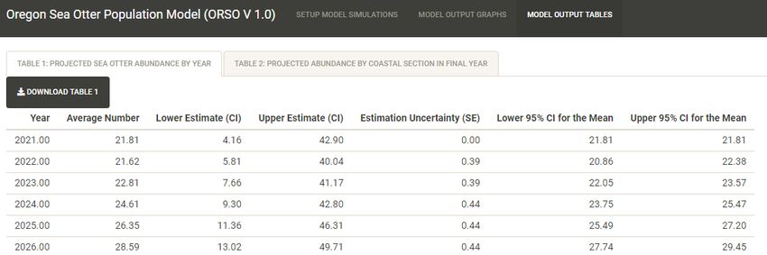
23MODEL OUTPUT TABLES Panel
The results of the simulation model can also be viewed in tabular form. After setting up and running
simulations, the user can navigate to “MODEL OUTPUT TABLES” panel, where two standardized tables
can be viewed and/or downloaded as *.csv files:
“Table 1: Projected Sea Otter Abundance by Year”
“Table 2: Projected Abundance by Coastal Section in Final Year”.
Table 1 summarizes total projected abundance across all of coastal Oregon for each year of the
simulation, and includes six metrics: average projected abundance, lower estimate 95% CI of the
projected abundance distribution, upper estimate 95% CI of the projected abundance distribution,
estimation uncertainty expressed by the standard error (SE) of the mean projected abundance, lower
95% CI for the average expected abundance, and upper 95% CI for the average expected abundance.
Table 2 summarizes the projected abundance and density in each coastal section on the final year of the
simulation: columns include area of benthic habitat in each section (km2), average projected number of
sea otters, lower estimate 95% CI of the projected abundance distribution, upper estimate 95% CI of the
projected abundance distribution, average density (number of sea otters/km2), lower 95% CI of the
projected density distribution, upper 95% CI of the projected density distribution.
In addition to viewing the tables, they can also be downloaded as csv files by clicking on the download
buttons above each table.
24References
Becker, S. L., T. E. Nicholson, K. A. Mayer, M. J. Murray, and K. S. Van Houtan. 2020. Environmental
factors may drive the post-release movements of surrogate-reared sea otters. Frontiers in
Marine Science 7.
Bodkin, J. L. 2015. Historic and Contemporary Status of Sea Otters in the North Pacific. Pages 43-61 in S.
Larson, J. L. Bodkin, and G. R. Vanblaricom, editors. Sea Otter Conservation. Academic Press,
Boston.
Bodkin, J. L., and B. E. Ballachey. 2010. Modeling the effects of mortality on sea otter populations. U.S.
Geological Survey Scientific Investigations Report. 2010–5096.
Bodkin, J. L., B. E. Ballachey, M. A. Cronin, and K. T. Scribner. 1999. Population demographics and genetic
diversity in remnant and translocated populations of sea otters. Conservation Biology 13:1378-
1385.
Bodkin, J. L., B. E. Ballachey, T. A. Dean, A. K. Fukuyama, S. C. Jewett, L. McDonald, D. H. Monson, C. E.
O'Clair, and G. R. VanBlaricom. 2002. Sea otter population status and the process of recovery
from the 1989 'Exxon Valdez' oil spill. Marine Ecology-Progress Series 241:237-253.
Breed, G. A., E. A. Golson, and M. T. Tinker. 2017. Predicting animal home-range structure and
transitions using a multistate Ornstein-Uhlenbeck biased random walk. Ecology 98:32-47.
Burn, D. M., A. M. Doroff, and M. T. Tinker. 2003. Carrying Capacity and pre-decline abundance of sea
otters (Enhydra lutris kenyoni) in the Aleutian Islands. Northwestern Naturalist 84:145-148.
Carswell, L. P. 2008. How Do Behavior and Demography Determine the Success of Carnivore
Reintroductions? A Case Study of Southern Sea Otters, Enhydra Lutris Nereis, Translocated to
San Nicholas Island. University of California, Santa Cruz.
Caswell, H. 2001. Matrix population models: construction, analysis, and interpretation. 2nd ed edition.
Sinauer Associates, Sunderland, MA.
Eberhardt, L. L., and K. B. Schneider. 1994. Estimating sea otter reproductive rates. Marine Mammal
Science 10:31-37.
Esslinger, G. G., and J. L. Bodkin. 2009. Status and trends of sea otter populations in Southeast
Alaska,1969–2003. U.S. Geological Survey Scientific Investigations Report 2009-5045., Reston,
VA.
Estes, J. A. 1990. Growth and equilibrium in sea otter populations. Journal of Animal Ecology 59:385-
402.
Garshelis, D. L. 1997. Sea otter mortality estimated from carcasses collected after the Exxon Valdez oil
spill. Conservation Biology 11:905-916.
Gelfand, A. E., and P. Vounatsou. 2003. Proper multivariate conditional autoregressive models for spatial
data analysis. Biostatistics 4:11-15.
Gerber, L. R., T. Tinker, D. Doak, and J. Estes. 2004. Mortality sensitivity in life-stage simulation analysis:
A case study of southern sea otters. Ecological Applications 14:1554–1565.
Gregr, E. J., L. M. Nichol, J. C. Watson, J. K. B. Ford, and G. M. Ellis. 2008. Estimating Carrying Capacity for
Sea Otters in British Columbia. The Journal of Wildlife Management 72:382-388.
Hughes, B. B., K. Wasson, M. T. Tinker, S. L. Williams, L. P. Carswell, K. E. Boyer, M. W. Beck, R. Eby, R.
Scoles, M. Staedler, S. Espinosa, M. Hessing-Lewis, E. U. Foster, K. M. Beheshti, T. M. Grimes, B.
H. Becker, L. Needles, J. A. Tomoleoni, J. Rudebusch, E. Hines, and B. R. Silliman. 2019. Species
recovery and recolonization of past habitats: lessons for science and conservation from sea
otters in estuaries. PeerJ 7:e8100.
Jameson, R. J. 1989. Movements, home range, and territories of male sea otters off central California.
Marine Mammal Science 5:159-172.
25Jameson, R. J., K. W. Kenyon, A. M. Johnson, and H. M. Wight. 1982. History and status of translocated
sea otter populations in North America. Wildl. Soc. Bull. 10:100-107.
Kone, D., M. T. Tinker, and L. Torres. in press. Informing sea otter reintroduction through habitat and
human interaction assessment. Endangered Species Research
https://doi.org/10.3354/esr01101.
Laidre, K. L., R. J. Jameson, and D. P. DeMaster. 2001. An estimation of carrying capacity for sea otters
along the California coast. Marine Mammal Science 17:294-309.
Laidre, K. L., R. J. Jameson, E. Gurarie, S. J. Jeffries, and H. Allen. 2009. Spatial Habitat Use Patterns of
Sea Otters in Coastal Washington. Journal of Mammalogy 90:906-917.
Laidre, K. L., R. J. Jameson, S. J. Jeffries, R. C. Hobbs, C. E. Bowlby, and G. R. VanBlaricom. 2002.
Estimates of carrying capacity for sea otters in Washington state. Wildlife Society Bulletin
30:1172-1181.
Lubina, J. A., and S. A. Levin. 1988. The spread of a reinvading species: Range expansion in the California
sea otter. American Naturalist 131:526-543.
Miller, M. A., M. E. Moriarty, L. Henkel, M. T. Tinker, T. L. Burgess, F. I. Batac, E. Dodd, C. Young, M. D.
Harris, D. A. Jessup, J. Ames, and C. Johnson. 2020. Predators, Disease, and Environmental
Change in the Nearshore Ecosystem: Mortality in southern sea otters (Enhydra lutris nereis)
from 1998-2012. Frontiers in Marine Science 7:582.
Monson, D. H., and A. R. Degange. 1995. Reproduction, preweaning survival, and survival of adult sea
otters at Kodiak Island, Alaska. Canadian Journal of Zoology 73:1161-1169.
Monson, D. H., D. F. Doak, B. E. Ballachey, A. Johnson, and J. L. Bodkin. 2000a. Long-term impacts of the
Exxon Valdez oil spill on sea otters, assessed through age-dependent mortality patterns.
Proceedings of the National Academy of Sciences of the United States of America 97:6562-6567.
Monson, D. H., J. A. Estes, J. L. Bodkin, and D. B. Siniff. 2000b. Life history plasticity and population
regulation in sea otters. Oikos 90:457-468.
Morris, W. F., and D. F. Doak. 2002. Quantitative Conservation Biology: Theory and Practice of
Population Viability Analysis. Sinauer.
Siniff, D. B., and K. Ralls. 1991. Reproduction, survival and tag loss in California sea otters. Marine
Mammal Science 7:211-229.
Staedler, M. M. 2011. Individual variation in maternal care and provisioning in the southern sea otter
(Enhydra lutris nereis): causes and consequences of diet specialization in a top predator.
Masters Thesis. University of California, Santa Cruz.
Tarjan, L. M., and M. T. Tinker. 2016. Permissible Home Range Estimation (PHRE) in Restricted Habitats:
A New Algorithm and an Evaluation for Sea Otters. PLoS One 11:e0150547.
Tinker, M. T. 2015. The Use of Quantitative Models in Sea Otter Conservation. Pages 257-300 in S.
Larson, J. L. Bodkin, and G. R. Vanblaricom, editors. Sea Otter Conservation. Academic Press,
Boston, MA.
Tinker, M. T., D. F. Doak, and J. A. Estes. 2008. Using demography and movement behavior to predict
range expansion of the southern sea otter. Ecological Applications 18:1781-1794.
Tinker, M. T., D. F. Doak, J. A. Estes, B. B. Hatfield, M. M. Staedler, and J. L. Bodkin. 2006. Incorporating
diverse data and realistic complexity into demographic estimation procedures for sea otters.
Ecological Applications 16:2293-2312.
Tinker, M. T., V. A. Gill, G. G. Esslinger, J. L. Bodkin, M. Monk, M. Mangel, D. H. Monson, W. E. Raymond,
and M. Kissling. 2019a. Trends and Carrying Capacity of Sea Otters in Southeast Alaska. Journal
of Wildlife Management 83:1073-1089.
Tinker, M. T., J. Tomoleoni, N. LaRoche, L. Bowen, A. K. Miles, M. Murray, M. Staedler, and Z. Randell.
2017. Southern sea otter range expansion and habitat use in the Santa Barbara Channel,
California. OCS Study BOEM 2017-002. U.S. Geological Survey Open File Report No. 2017-1001.
26Tinker, M. T., J. A. Tomoleoni, B. P. Weitzman, M. Staedler, D. Jessup, M. J. Murray, M. Miller, T. Burgess,
L. Bowen, A. K. Miles, N. Thometz, L. Tarjan, E. Golson, F. Batac, E. Dodd, E. Berberich, J. Kunz, G.
Bentall, J. Fujii, T. Nicholson, S. Newsome, A. Melli, N. LaRoche, H. MacCormick, A. Johnson, L.
Henkel, C. Kreuder-Johnson, and P. Conrad. 2019b. Southern sea otter (Enhydra lutris nereis)
population biology at Big Sur and Monterey, California --Investigating the consequences of
resource abundance and anthropogenic stressors for sea otter recovery. US Geological Survey
Open-File Report No. 2019-1022. US Geological Survey Open-File Report, Reston, VA.
Tinker, M. T., J. L. Yee, K. L. Laidre, B. B. Hatfield, M. D. Harris, J. A. Tomoleoni, T. W. Bell, E. Saarman, L.
P. Carswell, and A. K. Miles. 2021. Habitat features predict carrying capacity of a recovering
marine carnivore. Journal of Wildlife Management 85:303-323.
Udevitz, M. S., B. E. Ballachey, and D. L. Bruden. 1996. A population model for sea otters in Western
Prince William Sound. Exxon Valdez Oil Spill Restoration Project Final Report: Sea otter
demographics. 93043-3, U.S. National Biological Service, Alaska Science Center, Anchorage,
Alaska.
USFWS. 2013. Southwest Alaska Distinct Population Segment of the Northern sea otter (Enhydra lutris
kenyoni) - Recovery Plan., U.S. Fish and Wildlife Service, Region 7, Alaska, Anchorage, AK.
Williams, P. J., M. B. Hooten, J. N. Womble, G. G. Esslinger, M. R. Bower, and T. J. Hefley. 2017. An
integrated data model to estimate spatiotemporal occupancy, abundance, and colonization
dynamics. Ecology 98:328-336.
27You can also read