A Similarity-preserving Neural Network Trained on Transformed Images Recapitulates Salient Features of the Fly Motion Detection Circuit
←
→
Page content transcription
If your browser does not render page correctly, please read the page content below
A Similarity-preserving Neural Network Trained on
                                             Transformed Images Recapitulates Salient Features
                                                     of the Fly Motion Detection Circuit

                                                     Yanis Bahroun †       Anirvan M. Sengupta †‡    Dmitri B. Chklovskii†∗
                                                     †                    ‡                    ∗
arXiv:2102.05503v1 [cs.NE] 10 Feb 2021

                                                       Flatiron Institute Rutgers University NYU Langone Medical Center
                                                   {ybahroun,dchklovskii}@flatironinstitute.org, anirvans@physics.rutgers.edu,

                                                                                        Abstract

                                                  Learning to detect content-independent transformations from data is one of the
                                                  central problems in biological and artificial intelligence. An example of such prob-
                                                  lem is unsupervised learning of a visual motion detector from pairs of consecutive
                                                  video frames. Rao and Ruderman formulated this problem in terms of learning
                                                  infinitesimal transformation operators (Lie group generators) via minimizing image
                                                  reconstruction error. Unfortunately, it is difficult to map their model onto a biologi-
                                                  cally plausible neural network (NN) with local learning rules. Here we propose a
                                                  biologically plausible model of motion detection. We also adopt the transformation-
                                                  operator approach but, instead of reconstruction-error minimization, start with a
                                                  similarity-preserving objective function. An online algorithm that optimizes such
                                                  an objective function naturally maps onto an NN with biologically plausible learn-
                                                  ing rules. The trained NN recapitulates major features of the well-studied motion
                                                  detector in the fly. In particular, it is consistent with the experimental observation
                                                  that local motion detectors combine information from at least three adjacent pixels,
                                                  something that contradicts the celebrated Hassenstein-Reichardt model.

                                         1    Introduction

                                         Humans can recognize objects, such as human faces, even when presented at various distances, from
                                         various angles and under various illumination conditions. Whereas the brain performs such a task
                                         almost effortlessly, this is a challenging unsupervised learning problem. Because the number of
                                         training views for any given face is limited, such transformations must be learned from data com-
                                         prising different faces, or in a content-independent manner. Therefore, learning content-independent
                                         transformations plays a central role in reverse engineering the brain and building artificial intelligence.
                                         Perhaps the simplest example of this task is learning a visual motion detector, which computes the
                                         optic flow from pairs of consecutive video frames regardless of their content. Motion detector learning
                                         was addressed by Rao and Ruderman [32] who formulated this problem as learning infinitesimal
                                         translation operators (or generators of the translation Lie group). They learned a motion detector by
                                         minimizing, for each pair of consecutive video frames, the squared mismatch between the observed
                                         variation in pixel intensity values and that predicted by the scaled infinitesimal translation operator.
                                         Whereas such an approach learns the operators and evaluates transformation magnitudes correctly
                                         [32, 23, 44], its biological implementation has been lacking (see below).
                                         The non-biological nature of the neural networks (NNs) derived from the reconstruction approach has
                                         been previously encountered in the context of discovery of latent degrees of freedom, e.g. dimension-
                                         ality reduction and sparse coding [8, 27]. When such NNs are derived from the reconstruction-error-
                                         minimization objective they require non-local learning rules, which are not biologically plausible. To

                                         33rd Conference on Neural Information Processing Systems (NeurIPS 2019), Vancouver, Canada.
overcome this, [29, 30, 31] proposed deriving NNs from objectives that strive to preserve similarity
between pairs of inputs in corresponding outputs.
Inspired by [30, 31], we propose a similarity-preserving objective for learning infinitesimal translation
operators. Instead of preserving similarity of input pairs as was done for dimensionality reduction
NNs, our objective function preserves the similarity of input features formed by the outer product
of variation in pixel intensity and pixel intensity which are suggested by the translation-operator
formalism. Such objective is optimized by an online algorithm that maps onto a biologically plausible
NN. After training the similarity-preserving NN on one-dimensional (1D) and two-dimensional (2D)
translations, we obtain an NN that recapitulates salient features of the fly motion detection circuit.
Thus, our main contribution is the derivation of a biologically plausible NN for learning content-
independent transformations by similarity preservation of outer product input features.
1.1 Contrasting reconstruction and similarity-preservation NNs
We start by reviewing the NNs for discovery of latent degrees of freedom from principled objective
functions. Although these NNs do not detect transformations, they provide a useful analogy that
will be important for understanding our approach. First, we explain why the NNs derived from
minimizing the reconstruction error lack biological plausibility. Then, we show how the NNs derived
from similarity preservation objectives solve this problem.
To introduce our notation, the input to the NN is a set of vectors, xt ∈ Rn , t = 1, . . . , T , with
components represented by the activity of n upstream neurons at time, t. In response, the NN outputs
an activity vector, yt ∈ Rm , t = 1, . . . , T , where m is the number of output neurons.
The reconstruction approach starts with minimizing the squared reconstruction error:
X T h
X i
2
min ||xt − Wyt ||2 = min kxt k − 2x> > >
t Wyt + yt W Wyt , (1)
W,yt=1...T ∈Rm W,yt=1...T ∈Rm
t t=1
possibly subject to additional constraints on the latent variables yt or on the weights W ∈ Rn×m .
Without additional constraints, this objective is optimized offline by a projection onto the principal
subspace of the input data, of which PCA is a special case [25].
In an online setting, the objective can be optimized by alternating minimization [27]. After the arrival
of data sample, xt : firstly, the objective (1) is minimized with respect to the output, yt , while the
weights, W, are kept fixed, secondly, the weights are updated according to the following learning
rule derived by a gradient descent with respect to W for fixed yt :
> >
ẏt = Wt−1 xt − Wt−1 Wt−1 yt , Wt ←− Wt−1 + η (xt − Wt−1 yt ) yt> , (2)
In the NN implementations of the algorithm (2), the elements of matrix W are represented by synaptic
weights and principal components by the activities of output neurons yj , Fig. 1a [24].
However, implementing update (2)right in the single-layer NN architecture, Fig. 1a, requires non-
local learning rules making it biologically implausible. Indeed, the last term in (2)right implies that
updating the weight of a synapse requires the knowledge of output activities of all other neurons which
>
are not available to the synapse. Moreover, the matrix of lateral connection weights, −Wt−1 Wt−1 ,
in the last term of (2)left is computed as a Gramian of feedforward weights; a non-local operation.
This problem is not limited to PCA and arises in nonlinear NNs as well [27, 19].
Whereas NNs with local learning rules have been proposed [27] their two-layer feedback architecture
is not consistent with most biological sensory systems with the exception of olfaction [17]. Most
importantly, such feedback architecture seems inappropriate for motion detection which requires
speedy processing of streamed stimuli.
To address these difficulties, [30] derived NNs from similarity-preserving objectives. Such objectives
require that similar input pairs, xt and xt0 , evoke similar output pairs, yt and yt0 . If the similarity of
a pair of vectors is quantified by their scalar product, one such objective is similarity matching (SM):
T
X
min 1
2 (xt · xt0 − yt · yt0 )2 . (3)
∀t∈{1,...,T }: yt ∈Rm
t,t0 =1
2This offline optimization problem is also solved by projecting the input data onto the principal
subspace [46, 5, 20]. Remarkably, the optimization problem (3) can be converted algebraically to a
tractable form by introducing variables W and M [31]:
XT
T
min min max [ (−2x> > >
t Wyt +yt Myt )+T Tr(W W)− Tr(M> M)]. (4)
{yt ∈Rm }T
t=1
W∈R n×m M∈Rm×m
t=1
2
In the online setting, first, we minimize (4) with respect to the output variables, yt , by gradient
descent while keeping W, M fixed [30]:
ẏt = W> xt − Myt . (5)
To find yt after presenting the corresponding input, xt , (5) is iterated until convergence. After the
convergence of yt , we update W and M by gradient descent and gradient ascent respectively [30]:
Wij ← Wij + η (xi yj − Wij ) , Mij ← Mij + η (yi yj − Mij ) . (6)
Algorithm (5), (6) can be implemented by a biologically plausible NN, Fig. 1b. As before, activity
(firing rate) of the upstream neurons encodes input variables, xt . Output variables, yt , are computed
by the dynamics of activity (5) in a single layer of neurons. The elements of matrices W and M
are represented by the weights of synapses in feedforward and lateral connections respectively. The
learning rules (6) are local, i.e. the weight update, ∆Wij , for the synapse between ith input neuron
and j th output neuron depends only on the activities, xi , of ith input neuron and, yj , of j th output
neuron, and the synaptic weight. Learning rules (6) for synaptic weights W and −M (here minus
indicates inhibitory synapses, see Eq.(5)) are Hebbian and anti-Hebbian respectively.
A B
x1
A B AC B
(a) x1 (b) x1 (c) x1x x y1
2
x2 y1 x2 y1 x2x y1
-M
...
...
-M -M
...
...
- WTW ...
...
...
yk
...
...
...
yk yk yk
xn W
xn W xn W xnx W
Hebbian anti-Hebbian synapses
Non-local Hebbian anti-Hebbian synapses Hebbian
Principal anti-Hebbian synapses
Rectification
Rectification
Figure 1: Single-layer NNs performing online (a) reconstruction error minimization (1) [24, 27], (b)
similarity matching (SM) (3) [30], and (c) nonnegative similarity matching (NSM) (7) [29].
We now compare the objective functions of the two approaches. After dropping invariant terms, the
reconstructive objective function has the following interactions among input and output variables:
−2x> > > > >
t Wyt + yt W Wyt (Eq 1). The SM approach leads to −2xt Wyt + yt Myt , ( Eq 4). The
term linear in yt , a cross-term between inputs and outputs, −2x>t Wy t , is common in both approaches
and is responsible for projecting the data onto the principal subspace via the feedforward connections
in Fig.1ab. The terms quadratic in yt ’s decorrelate different output channels via a competition
implemented by the lateral connections in Fig.1ab and are different in the two approaches. In
particular, the inhibitory interaction between neuronal activities yj in the reconstruction approach
depends upon W> W, which is tied to trained W in a non-local way. In contrast, in the SM approach
the inhibitory interaction matrix M is learned for yj ’s via a local anti-Hebbian rule.
The SM approach can be applied to other computational tasks such as clustering and learning
manifolds by tiling them with localized receptive fields [35]. To this end we modify the offline
optimization problem (3) by constraining the output, yt ∈ Rm
+ , which represents assignment indices
(as e.g. in the K-means algorithm):
T
X
min 1
2 (xt · xt0 − yt · yt0 )2 . (7)
∀t∈{1,...,T }: yt ∈Rm
+
t,t0 =1
Such nonnegative SM (NSM), just like the optimization problem (3), (7) can be converted alge-
braically to a tractable form by introducing similar variables W and M [29]. The synaptic weight
update rules presented in (6) remain unchanged and the only difference between the online solutions
of (3) and (7) is the dynamics of neurons which, instead of being linear, are now rectifying, Fig. 1c.
3In the next section, we will address transformation learning. Similarly, we will review the recon-
struction approach, identify the key term analogous to the cross-term −2x> t Wyt , and then alter the
objective function, so that the cross-term is preserved but the inhibition between output neurons can
be learned in a biologically plausible manner.
2 Learning a motion detector using similarity preservation
Now, we focus on learning to detect transformations from pairs of consecutive video frames, xt , and
xt+1 . We start with the observation that much of the change in pixel intensities in consecutive frames
arises from a translation of the image. For infinitesimal translations, pixel intensity change is given by
a linear operator (or matrix), denoted by Aa , multiplying the vector of pixel intensity scaled by the
magnitude of translation, denoted by θa . Because for a 2D image multiple directions of translation
are possible, there is a set of translation matrices with corresponding magnitudes. Our goal is to learn
both the translation matrices from pairs of consecutive video frames and compute the magnitudes of
translations for each pair. Such a learning problem will reduce to the one discussed in the previous
section, but performed on an unusual feature – the outer product of pixel intensity and variation of
pixel intensity vectors.
2.1 Reconstruction-based transformation learning
We represent a video frame at time, t, by the pixel intensity vector, xt , formed by reshaping an image
matrix into a vector. For infinitesimal transformations, the difference, ∆xt , between two consecutive
frames, xt and xt+1 is:
K
X
∆xt = xt+1 − xt = θta Aa xt , ∀t ∈ {1, . . . , T − 1}. (8)
a=1
where, for each transformation, a ∈ {1, . . . K}, between the frames, t and t + 1, we define a
transformation matrix Aa and a magnitude of transformations, θta . Whereas for image translation
Aa is known to implement a spatial derivative operator, we are interested in learning Aa from data in
unsupervised fashion.
Previously, unsupervised algorithms for learning both Aa and θta were derived by minimizing with
respect to Aa and θta the prediction-error squared [32] where optimal Aa and θta minimize the
mismatch between the actual image and the one computed based on the learned model:
X K
X Xh K
X K
X i
k∆xt − θta Aa xt k2 = k∆xt k2 − 2∆x>
t θta Aa xt + k θta Aa xt k2 . (9)
t a=1 t a=1 a=1
Whereas solving (9) in the offline setting leads to reasonable estimates of Aa and θta [32], it is rather
non-biological. In a biologically plausible online setting the data are streamed sequentially and θta
(Aa ) must be computed (updated) with minimum latency. The algorithm can store only the latest
pair of images and a small number of variables, i.e. sufficient statistic, but not any significant part of
the dataset. Although a sketch of neural architecture was proposed in [32], it is clear from Section
1.1 that due to the quadratic term in the output, θta , a detailed architecture will suffer from the same
non-locality as the reconstruction approach to latent variable NNs (1).
As the cross-term in (9) plays a key role in projecting the data (Section 1.1), we re-write it as follows:
X K
X X X X
∆x>
t θta Aa xt = ∆xt,i θta Aai,j xt,j = θta Aai,j ∆xt,i xt,j = Θt AVec(∆xt x>
t ) , (10)
t a=1 i,j,t,a i,j,t,a t
2
where we introduced A ∈ RK×n , the matrix whose components represents the vectorized version
a={1...K} >
of the generators, Aa,: = Vec(Aa ), ∀a ∈ {1, . . . , K} and Θt = (θt ) , the vector whose
components represent the magnitude of the transformation, a, at time, t.
Eq. (10) shows that the cross-term favors aligning Aa,: in the direction of the outer product of pixel
intensity variation and pixel intensity vectors, Vec(∆xx> ). Although central to the learning of
transformations in (9), the outer product of pixel intensity variation and pixel intensity vectors was
not explicitly highlighted in the transformation-operator learning approach [32, 10, 23].
42.2 Why the outer product of pixel intensity variation and pixel intensity vectors?
Here, we provide intuitions for using outer products in content-independent detection of translations.
For simplicity, we consider 1D motion in a 1D world. Motion detection relies on a correspondence
between consecutive video frames, xt and xt+1 .
One may think that such correspondences can be detected by a neuron adding up responses of the
displaced filters applied to xt and xt+1 . While possible in principle, such neuron’s response would
be highly dependent on the image content [21, 22]. This is because summing the outputs of the two
filters amounts to applying an OR operation to them which does not selectively respond to translation.
To avoid such dependence on the content, [21] proposed to invoke an AND operation, which is
implemented by multiplication. Specifically, consider forming an outer product of xt and xt+1 and
summing its values along each diagonal. If the image is static then the main diagonal produces
the highest correlation. If the image is shifted by one pixel between the frames then the first
sub(super)-diagonal yields the highest correlation. If the image is shifted by two pixels - the second
sub(super)-diagonal yields the highest correlation and so on. Then, if the sum over each diagonal
is represented by a different neuron, the velocity of the object is given by the most active neuron.
Other models relying on multiplications are "mapping units" [15], "dynamic mappings" [43] and
other bilinear models [26].
Our algorithm for motion detection adopts multiplication to detect correspondences but computes an
outer product between the vectors of pixel intensity, xt , and pixel intensity variation, ∆xt . Compared
to the approach in [21], one advantage of our approach is that we do not require separate neurons to
represent different velocities but rather have a single output neuron (for each direction of motion),
whose activity increases with velocity. Previously, a similar outer product feature was proposed in
[3] (for a formal connection - see Supplement A). Another advantage of our approach is a derivation
from the principled SM objective motivated by the transformation-operator formalism.
2.3 A novel similarity matching objective for learning transformations
Having identified the cross-term in (9) analogous to that in (1), we propose a novel objective function
where the inhibition between output neurons is learned in a biologically plausible manner. By analogy
with (Eq.3), we substitute the reconstruction-error-minimization objective by an SM objective for
2
transformation learning. We denote the vectorized outer product between ∆xt and xt as χt ∈ Rn :
χt,α = (∆xt x>
t )i,j , with α = (i − 1)n + j, (11)
We concatenate these vectors into a matrix, χ ≡ [χ1 , . . . , χT ], as well as the transformation magni-
tude vectors, Θ ≡ [Θ1 , . . . , ΘT ]. Using these notations, we introduce the following SM objective:
T T
1 XX >
min kχ> χ − Θ> Θk2F = min (χt χt0 − Θ> 2
t Θt0 ) . (12)
Θ∈RK×T Θ1 ,...,ΘT T2 t 0
t
To reconcile (9) and (12), we first show that the cross-terms are the same by introducing the following
2
optimization over a matrix, W ∈ RK×n as:
T T T
" T # T
1 XX > > 1 X > X > 2X >
Θ t Θ 0 χ
t t t χ 0 = Θ Θ 0 χ
t t0 χ t = max Θt Wχt − TrW> W (13)
T 2 t=1 0 T 2 t=1 t 0 W T
t=1
t =1 t =1
Therefore, the SM approach yields the cross-term, Θ> >
t Wχt which is the same as Θt AVec(∆xt xt )
>
a
in [32]. We can thus identify the rows Wa,: with the vectorized transformation matrices, Vec(A ),
Fig. 2a. Solutions of (12) are known to be projections onto the principal subspace of χ, the vectorized
outer product of ∆xt and xt which are equivalent, up to an orthogonal rotation, to PCA.
If we constrain the output to be nonnegative (NSM):
min kχ> χ − Θ> Θk2F . (14)
Θ∈RK×T
+
then by analogy with Sec. 1.1 [29], this objective function clusters data or tiles data manifolds [35].
52.4 Online algorithm and NN
To derive online learning algorithms for (12) and (14) we follow the similarity matching approach [30].
The optimality condition of each online problem is given by [29, 30] for SM and NSM respectively:
SM: Θ∗t = Wχt − MΘ∗t ; NSM: Θ∗t = max(Wχt − MΘ∗t , 0) , (15)
2
with W and M found using recursive formulations, ∀a ∈ {1, . . . , K}, ∀α ∈ {1, . . . , n }:
Waα ← Waα + Θt−1,a (χt−1,α − Waα Θt−1,a ) Θ̂t,a (16)
Maa0 6=a ← Maa0 + Θt−1,a (Θt−1,a0 − Maa0 Θt−1,a ) Θ̂t,a (17)
Θ̂t,a = Θ̂t−1,a + (Θt−1,a )2 . (18)
This algorithm is similar to the model proposed in [30], but it is more difficult to implement in
a biologically plausible way. This is because χt is an outer product of input data and cannot be
identified with the inputs to a single neuron. To implement this algorithm, we break up W into rank-1
components, each of which is computed in a separate neuron such that:
X X X
Θ∗t,a = ∆xt,i Wija xt,j − Maa0 Θ∗t,a0 . (19)
i j a0
Each element of the tensor, Wija will be encoded in the weight of a feedforward synapse from
the j-th pixel onto i-th neuron encoding a-th transformation (see Fig. 2a). Biologically plausible
implementations of this algorithm are given in Section 3.
2.5 Numerical experiments
Here, we implement the biologically plausible algorithms presented in the previous subsection and
report the learned transformation matrices. To validate the results of SM and NSM applied to the
outer-product feature, χ, we compare them with those of PCA and K-means, respectively, also applied
to χ as formally defined in in Supplement B. These standard but biologically implausible algorithms
were chosen because they perform similar computations in the context of latent variable discovery.
The 1D visual world is represented by a continuous profile of light intensity as a function of one
coordinate. A 1D eye measures light intensity in a 1D window consisting of n discrete pixels. To
imitate self-motion, such window can move left and right by a fraction of a pixel at each time step.
For the purpose of evaluating the proposed algorithms and derived NNs, we generated artificial
training data by subjecting a randomly generated 1D image (Gaussian, exponentially correlated noise)
to known horizontal subpixel translations. Then, we spatially whitened the discrete images by using
the ZCA whitening technique [2].
We start by learning K = 2 transformation matrices using each algorithm. After the rows of the
synaptic weights, W, are reshaped into n × n matrices, they can be identified with the transformation
operators, A. Then the magnitude of the transformation given by ∆x> t Axt , Fig. 2a.
SM and PCA. The filters learned from SM are shown in Fig.2c and those learned from PCA - in
Fig.2e. The left panels of Fig.2ce represent the singular vectors capturing the maximum variance.
They replicate the known operator of translation, a spatial derivative, found in [32]. The right panels
of Fig.2ce show the singular vector capturing the second largest variance, which do not account for a
known transformation matrix. In the absence of a nonnegativity constraint a reversal of translation is
represented by a change of sign of the transformation magnitude.
NSM and K-means. The filters learned by NSM are shown in Fig.2d and those learned by K-means
- in Fig. 2f. They are similar to the first singular vector learned by SM, PCA and [32]. However, in
NSM and K-means the output must be nonnegative, so representing the opposite directions of motion
requires two filters, which are sign inversions of each other.
For the various models, the rows of the learned operators, Aa , are identical except for a shift, i.e. the
same operator is applied at each image location. As expected, the learned filters compute a spatial
derivative of the pixel intensity, red rectangle in Fig.2a. The learned weights can be approximated by
61th Principal Component 2th Principal Component
W+,: x",& − x",% x!,# x!,$ x!,%
x",% ≈ [Δx",& Δx",% Δx",' Δx",( Δx",)] x",&-x",'
x &
[Δx",& Δx",% Δx",' Δx",( Δx",)] x",%-x",(
x",' &'
+ -
x",( x",'−x",)
(a) x",) x",( (b)
x",: Δx!,# ×(x!,# −x!,% )
Δx",:
3th Principal Component 4th Principal Component
(c) (d) (e) (f)
Figure 2: The rows of the synaptic weight matrix Wa,: are reshaped into n × n transformation
matrices Aa . Then, the magnitude of the transformation is ∆x> a
t A xt . Such a computation can be
approximated by the cartoon model (b). Synaptic weights learned from 1D translation on a vector of
size 5 pixels by (c) SM, (d) NSM, (e) PCA (decreasing eigenvalues), and (f) K-means.
the filter keeping only the three central pixels, Fig.2 which we name the cartoon model of the motion
detector. It computes a correlation between the spatial derivative denoted by ∆i xt,i and the temporal
derivative, ∆t xt . Such algorithm may be viewed as a Bayesian optimal estimate of velocity in the
low SNR regime (Supplement C) appropriate for the fly visual system[38].
The results presented in Fig.2 were obtained with n = 5 pixels, but the same structure was observed
with larger values of n. Similar results were also obtained with models trained on moving periodic
sine-wave gratings often used in fly experiments.
We also trained our NN on motion in the four cardinal directions, and planar rotations of two-
dimensional images as was done in [32] and showed that our model can learn such transformations.
By using NSM we can again distinguish between motion in the four cardinal directions, and clockwise
and counterclockwise rotations, which was not possible with prior approaches (see Supplement D).
3 Learning transformations in a biologically plausible way
In this section, we propose two biologically plausible implementations of a motion detector by taking
advantage of the decomposition of the outer product feature matrix into single-row components (19).
The first implementation models computation in a mammalian neuron such as a cortical pyramidal
cell. The second models computation in a Drosophila motion-detecting neuron T4 (same arguments
apply to T5). In the following, for simplicity we focus on the cartoon model Fig.2b.
3.1 Multi-compartment neuron model
Mammalian neurons can implement motion computation by representing each row of the trans-
formation matrix, W, in a different dendritic branch originating from the soma (cell body). Each
such branch forms a compartment with its own membrane potential [14, 39] allowing it to perform
its own non-linear computation the results of which are then summed in the soma. Each dendrite
compartment receives pixel intensity variation from only one pixel via a proximal shunting inhibitory
synapse [42, 16] and the pixel intensity vector via more distal synapses, Fig. 3a. We assume that
the conductance of the shunting inhibitory synapse decreases with the variation in pixel intensity.
The weights of the more distal synapses represent the corresponding row of the outer product feature
matrix. When the variation in pixel intensity is low, the shunting inhibition vetoes other post-synaptic
currents. When the variation in pixel intensity is high, the shunting is absent and the remaining
post-synaptic currents flow into the soma. A formal analysis shows that this operation can be viewed
as a multiplication [42, 16]. Different compartments compute such products for variation in intensity
of different pixels, after which these products are summed in the soma (19), Fig. 3a.
The weight of a distal synapse is updated using a Hebbian learning rule applied to the corresponding
pixel intensity available pre-synaptically and the transformation magnitude modulated by the shunting
inhibition representing pixel intensity variation, Fig. 3b. The transformation magnitude is computed in
the soma and reaches distal synapses via backpropagating dendritic spikes [40]. Such backpropagating
signal is modulated by the shunting inhibition, thus implementing multiplication of the transformation
7magnitude and pixel intensity variation (16), Fig. 3b . Competition between the neurons detecting
motion in different directions is mediated by inhibitory interneurons [28].
Neural activity computed according to (19) Synaptic update by dendritic backpropagation
! ! !
Θ∗t,a = ∆xt,i Wija xt,j − Maa′ Θ∗t,a′ . according to (16-18)
i j a′
xi#' xi#'
xi#$ xi#$
xi xi
xi%$ xi%$
xi%' xi%'
∆xi%$ ∆xi%$
!"a !"a
(a) Soma (b) Soma
xi#' xi#$ xi xi%$ xi%' ∆xi xi#' xi#$ xi xi%$ xi%' ∆xi
Excitatory Inhibitory Shunting Dendritic
connection connection Inhibition Backpropagation
Figure 3: A multi-compartment model of a mammalian neuron. (a) Each dendrite multiplies pixel
intensity variation signaled by the shunting inhibitory synapse and the weighted vector of pixel
intensities carried by more distal synapses. Products computed in each dendrite are summed in the
soma to yield transformation magnitude encoded in the spike rate. (b) Synaptic weights are updated
by the product of the corresponding pre-synaptic pixel intensities and the backpropagating spikes
modulated by the shunting inhibition.
3.2 A learned similarity preserving NN replicates the structure of the fly motion detector
The Drosophila visual system comprises retinotopically organized layers of neurons, meaning that
nearby columns process photoreceptor signals (identified with xi below) from nearby locations
in the visual field. Unlike the implementation in the previous subsection, motion computation is
performed across multiple neurons. The local motion signal is first computed in each of the hundreds
of T4 neurons that jointly tile the visual field. Their outputs are integrated by the downstream giant
tangential neurons. Each T4 neuron receives light intensity variation from only one pixel via synapses
from neurons Mi1 and Tm3 and light intensities from nearby pixels via synapses from neurons Mi4
and Mi9 (with opposite signs) [41], Fig. 3c. Therefore, in each T4 neuron ∆x is a scalar and W is a
vector and local motion velocity can be computed by a single-compartment neuron. If the weights of
synapses from Mi4 and Mi9 of different columns represent W, then the multiplication of ∆x and
Wx can be accomplished as before using shunting inhibition. Competition among T4s detecting
different directions of motion is implemented by inhibitory lateral connections.
Pixel i − 1 Pixel i Pixel i + 1 Column i − 1 Column i Column i + 1
Column 1 Column 2 Column 3
∆xi%& xi%& ∆xi xi ∆xi'& xi'& Mi1/Tm3 Mi9 Mi4 Mi1/Tm3 Mi9 Mi4 Mi1/Tm3 Mi9 Mi4
Mi1/Tm3 Mi9 Mi4 Mi1/Tm3 Mi9 Mi4 Mi1/Tm3 Mi9 Mi4T4 right
EMD right T4
i i e e i i
- x +
i i e e i i
T4 left
(a) (b) (c)
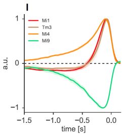
Figure 4: An NN trained on 1D translations recapitulates the motion detection circuit in Drosophila.
(a) Each motion-detecting neuron receives pixel intensity variation signal from pixel i and pixel
intensity signals at least from pixels i − 1 and i + 1 (with opposite signs). (b) In Drosophila, each
retinotopically organized column contains neurons Mi1/Tm3, Mi9, and Mi4 [41] which respond to
light intensity in the corresponding pixel according to the impulse responses shown in (c) (from [1]).
Each T4 neuron selectively samples different inputs from different columns [41]: it receives light
intensity variation via Mi1/Tm3 and light intensity via Mi4 and Mi9 (with opposite signs).
Our model correlates inputs from at least three pixels in agreement with recent experimental results
[41, 1, 11, 34], instead of two in the celebrated Hassenstein-Reichardt detector (HRD)[33]. In the
fly, outputs of T4s are summed over the visual field in downstream neurons. The summed output of
our detectors is equivalent to the summed output of HRDs and thus consistent with multiple prior
behavioral experiments and physiological recordings from downstream neurons (see Supplement E).
There is experimental evidence for both nonlinear interactions of T4 inputs [34, 13] supporting a
multiplicative model but also for the linear summation of inputs [11, 45]. Even if summation is linear,
the neuronal output nonlinearity can generate multiplicative terms for outer product computation.
8The main difference between our learned model (Fig.2a) and most published models is that the
motion detector is learned from data using biologically plausible learning rules in an unsupervised
setting. Thus, our model can generate somewhat different receptive fields for different natural image
statistics such as that in ON and OFF pathways potentially accounting for minor differences reported
between T4 and T5 circuits [41].
A recent model from [34] also uses inputs from three differently preprocessed inputs. Unlike our
model that relies on a derivative computation in the middle pixel, the model in [34] is composed of a
shared non-delay line flanked by two delay lines.
As shown in Supplement E, after integration over the visual field, the global signal from our cartoon
model Fig.2b is equivalent to that from HRD. Same observation has been made for the model in [34].
Yet, the predicted output of a single motion detector in our model is different from both HRD and
[34].
3.3 Experimentally established properties of the global motion detector
Until recently, most experiments confirmed the predictions of the HRD model. However, almost all
of these experiments measured either the activity of downstream giant neurons integrating T4 output
over the whole visual field or the behavioral response generated by these giant neurons. Because after
integration over the visual field, the global signal from our cartoon model Fig.2b is equivalent to that
from HRD, various experimental confirmations of the HRD predictions are inherited by our model.
Below, we list some of the confirmed predictions.
Dependence of the output on the image contrast. Because HRD multiplies signals from the two
photoreceptors its output should be quadratic in the stimulus contrast. Similarly, in our model, the
output should be proportional to contrast squared because it is given by the covariance between time
and space derivatives of the light intensity Supplement C each proportional to contrast. Note that
this prediction differs from [32] whose output is contrast-independent. Several experiments have
confirmed these predictions in the low SNR regime [12, 7, 9, 37, 4]. Of course, the output cannot
grow unabated and, in the high SNR regime, the output becomes contrast independent. A likely cause
is the signal normalization between photoreceptors and T4 [12].
Oscillations in the motion signal locked to the visual stimulus. In accordance with the oscillating
output of HRD in response to moving periodic stimulus, physiological recordings have reported such
phase-locked oscillations [6]. Our model reproduces such oscillations.
Dependence of the peak velocity on the wavelength. In our model, just like in the HRD, output
first increases with the velocity of the visual stimulus and then decreases. The optimal velocity is
proportional to the spatial wavelength of the visual stimulus because then the temporal frequency of
the optimal stimulus is a constant given by the inverse of the time delay in one of the arms.
In conclusion, we learn transformation matrices using a similarity-preserving approach leading to a
biologically plausible model of a motion detector. Generalizing our work to the learning of other
content-preserving transformation will open a path towards principled biologically plausible object
recognition.
Acknowledgments
We are grateful to P. Gunn, and A. Genkin for discussion and comments on this manuscript. We thank
D. Clark, J. Fitzgerald, E. Hunsicker, and B. Olshausen for helpful discussions.
References
[1] Alexander Arenz, Michael S Drews, Florian G Richter, Georg Ammer, and Alexander Borst.
The temporal tuning of the drosophila motion detectors is determined by the dynamics of their
input elements. Current Biology, 27(7):929–944, 2017.
[2] Anthony J Bell and Terrence J Sejnowski. The “independent components” of natural scenes are
edge filters. Vision research, 37(23):3327–3338, 1997.
[3] Matthias Bethge, Sebastian Gerwinn, and Jakob H Macke. Unsupervised learning of a steerable
basis for invariant image representations. In Human Vision and Electronic Imaging XII, volume
6492, page 64920C. International Society for Optics and Photonics, 2007.
9[4] Erich Buchner. Elementary movement detectors in an insect visual system. Biological cybernet-
ics, 24(2):85–101, 1976.
[5] Trevor F Cox and Michael AA Cox. Multidimensional scaling. Chapman and hall/CRC, 2000.
[6] Martin Egelhaaf and Alexander Borst. A look into the cockpit of the fly: visual orientation,
algorithms, and identified neurons. The Journal of Neuroscience, 13(11), 1993.
[7] G Fermi and W Reichardt. Optomotor reactions of the fly, musca domestica. dependence of
the reaction on wave length, velocity, contrast and median brightness of periodically moved
stimulus patterns. Kybernetik, 2:15–28, 1963.
[8] Peter Földiák. Learning invariance from transformation sequences. Neural Computation,
3(2):194–200, 1991.
[9] KG Götz. Optomoter studies of the visual system of several eye mutants of the fruit fly
drosophila. Kybernetik, 2(2):77, 1964.
[10] David B Grimes and Rajesh PN Rao. Bilinear sparse coding for invariant vision. Neural
computation, 17(1):47–73, 2005.
[11] Eyal Gruntman, Sandro Romani, and Michael B Reiser. Simple integration of fast excitation and
offset, delayed inhibition computes directional selectivity in drosophila. Nature neuroscience,
21(2):250, 2018.
[12] Juergen Haag, Winfried Denk, and Alexander Borst. Fly motion vision is based on reichardt
detectors regardless of the signal-to-noise ratio. Proceedings of the National Academy of
Sciences, 101(46):16333–16338, 2004.
[13] Juergen Haag, Abhishek Mishra, and Alexander Borst. A common directional tuning mechanism
of drosophila motion-sensing neurons in the on and in the off pathway. Elife, 6:e29044, 2017.
[14] Michael Häusser and Bartlett Mel. Dendrites: bug or feature? Current opinion in neurobiology,
13(3):372–383, 2003.
[15] Geoffrey F Hinton. A parallel computation that assigns canonical object-based frames of
reference. In Proceedings of the 7th international joint conference on Artificial intelligence-
Volume 2, pages 683–685. Morgan Kaufmann Publishers Inc., 1981.
[16] Christof Koch, Tomaso Poggio, and Vincent Torre. Nonlinear interactions in a dendritic tree:
localization, timing, and role in information processing. Proceedings of the National Academy
of Sciences, 80(9):2799–2802, 1983.
[17] Alexei A Koulakov and Dmitry Rinberg. Sparse incomplete representations: a potential role of
olfactory granule cells. Neuron, 72(1):124–136, 2011.
[18] Holger G Krapp and Roland Hengstenberg. Estimation of self-motion by optic flow processing
in single visual interneurons. Nature, 384(6608):463, 1996.
[19] Daniel D Lee and H Sebastian Seung. Learning the parts of objects by non-negative matrix
factorization. Nature, 401(6755):788–791, 1999.
[20] KV Mardia, JT Kent, and JM Bibby. Multivariate analysis. Academic press, 1980.
[21] Roland Memisevic. Learning to relate images: Mapping units, complex cells and simultaneous
eigenspaces. arXiv preprint arXiv:1110.0107, 2011.
[22] Roland Memisevic. Learning to relate images. IEEE Transactions on pattern analysis and
machine intelligence, 35(8):1829–1846, 2013.
[23] Xu Miao and Rajesh PN Rao. Learning the lie groups of visual invariance. Neural computation,
19(10):2665–2693, 2007.
[24] E Oja. Principal components, minor components, and linear neural networks. Neural Networks,
5(6):927–935, 1992.
[25] Erkki Oja. Simplified neuron model as a principal component analyzer. J. Math. Biol., 15(3):267–
273, 1982.
[26] Bruno A Olshausen, Charles Cadieu, Jack Culpepper, and David K Warland. Bilinear models
of natural images. In Human Vision and Electronic Imaging XII, volume 6492, page 649206.
International Society for Optics and Photonics, 2007.
10[27] Bruno A Olshausen and David J Field. Emergence of simple-cell receptive field properties by
learning a sparse code for natural images. Nature, 381:607–609, 1996.
[28] Cengiz Pehlevan and Dmitri Chklovskii. A normative theory of adaptive dimensionality
reduction in neural networks. In Advances in neural information processing systems, pages
2269–2277, 2015.
[29] Cengiz Pehlevan and Dmitri B Chklovskii. A Hebbian/anti-Hebbian network derived from
online non-negative matrix factorization can cluster and discover sparse features. In 2014 48th
Asilomar Conference on Signals, Systems and Computers, pages 769–775. IEEE, 2014.
[30] Cengiz Pehlevan, Tao Hu, and Dmitri B Chklovskii. A Hebbian/anti-Hebbian neural network
for linear subspace learning: A derivation from multidimensional scaling of streaming data.
Neural computation, 27(7):1461–1495, 2015.
[31] Cengiz Pehlevan, Anirvan M Sengupta, and Dmitri B Chklovskii. Why do similarity matching
objectives lead to Hebbian/anti-Hebbian networks? Neural Computation, 30(1):84–124, 2018.
[32] Rajesh PN Rao and Daniel L Ruderman. Learning lie groups for invariant visual perception. In
Advances in neural information processing systems, pages 810–816, 1999.
[33] Werner Reichardt. Autocorrelation, a principle for the evaluation of sensory information by the
central nervous system. Sensory communication, pages 303–317, 1961.
[34] Emilio Salazar-Gatzimas, Margarida Agrochao, James E Fitzgerald, and Damon A Clark. The
neuronal basis of an illusory motion percept is explained by decorrelation of parallel motion
pathways. Current Biology, 28(23):3748–3762, 2018.
[35] Anirvan Sengupta, Cengiz Pehlevan, Mariano Tepper, Alexander Genkin, and Dmitri Chklovskii.
Manifold-tiling localized receptive fields are optimal in similarity-preserving neural networks.
In Advances in Neural Information Processing Systems, pages 7080–7090, 2018.
[36] Eero Peter Simoncelli. Distributed representation and analysis of visual motion. PhD thesis,
Massachusetts Institute of Technology, 1993.
[37] Sandra Single and Alexander Borst. Dendritic integration and its role in computing image
velocity. Science, 281(5384):1848–1850, 1998.
[38] Shiva R Sinha, William Bialek, and Rob R van Steveninck. Optimal local estimates of visual
motion in a natural environment. arXiv preprint arXiv:1812.11878, 2018.
[39] Nelson Spruston. Pyramidal neurons: dendritic structure and synaptic integration. Nature
Reviews Neuroscience, 9(3):206, 2008.
[40] Greg Stuart, Nelson Spruston, Bert Sakmann, and Michael Häusser. Action potential initiation
and backpropagation in neurons of the mammalian cns. Trends in neurosciences, 20(3):125–131,
1997.
[41] Shin-ya Takemura, Aljoscha Nern, Dmitri B Chklovskii, Louis K Scheffer, Gerald M Rubin,
and Ian A Meinertzhagen. The comprehensive connectome of a neural substrate for ‘on’motion
detection in drosophila. Elife, 6, 2017.
[42] V Torre and T Poggio. A synaptic mechanism possibly underlying directional selectivity to mo-
tion. Proceedings of the Royal Society of London. Series B. Biological Sciences, 202(1148):409–
416, 1978.
[43] Christoph Von Der Malsburg. The correlation theory of brain function. In Models of neural
networks, pages 95–119. Springer, 1994.
[44] Jimmy Wang, Jascha Sohl-Dickstein, and Bruno Olshausen. Unsupervised learning of lie group
operators from image sequences. In Frontiers in Systems Neuroscience. Conference Abstract:
Computational and systems neuroscience, volume 1130, 2009.
[45] Carl FR Wienecke, Jonathan CS Leong, and Thomas R Clandinin. Linear summation underlies
direction selectivity in drosophila. Neuron, 99(4):680–688, 2018.
[46] Christopher KI Williams. On a connection between kernel pca and metric multidimensional
scaling. In Advances in neural information processing systems, pages 675–681, 2001.
11Supplementary Materials
This is the supplementary material for NeurIPS 2019 paper: "A Similarity-preserving Neural Network
Trained on Transformed Images Recapitulates Salient Features of the Fly Motion Detection Circuit"
by Y. Bahroun, A. M. Sengupta, and D. B. Chklovksii.
A Alternative features for learning transformations
As described in Section 2.2 (main text), our algorithm for motion detection adopts multiplication to
detect correspondences, it computes an outer product between the vectors of pixel intensity, xt , and
pixel intensity variation, ∆xt . Although an outer product feature was proposed in [21], our model
most resembles that of [3]. We show in the following that in the first order our model and that of [3]
are related.
Let us consider a mid-point in time between t and t + 1, denoted by t + 1/2. Using the same
approximation as before, xt+1/2 can be expressed as function of either xt or xt+1 as
1
= xt + θt Aa xt
xt+1/2 (20)
2
1
= xt+1 − θt Aa xt+1 (21)
2
By subtracting the two equations above we obtain
1
xt+1 − xt =θt Aa (xt+1 + xt ). (22)
2
We can thus rephrase the reconstruction error as:
X K
1X a a
mina k∆xt − θ A (xt+1 + xt )k2 (23)
θt ,A
t
2 a=1 t
leading to the cross-term θt Aa (xt+1 + xt )∆x> t , which corresponds to one proposed by [3]. An
interesting observation regarding the outer product (xt+1 + xt )∆x>t , is that, unlike the one used in
the main text, this feature has a time-reversal anti-symmetry. This helps detecting the direction of
change.
Another feature considered in [3] is
xt+1 x> >
t − xt xt+1 (24)
which exhibits an anti-symmetry both in time and in indices.
The anti-symmetric property of the learnable transformation operators is expected to arise from the
data rather than by construction. In fact, only elements of the algebra of SO(n) are anti-symmetric,
which, in all generality, constitute only a subset of all possible transformations in GL(n). Nevertheless,
we obtain again in the first order:
xt+1 x> >
t − xt xt+1 = (xt + θAxt )x>
t − xt (xt + θAxt )
>
= θAxt x> > >
t − (θAxt xt ) . (25)
B K-means and PCA for transformation learning
We proposed to evaluate the SM and NSM model for transformation learning in relation with
associated K-means and PCA models for transformation learning. The models are respectively
defined as the solution of the following optimization problems:
X
min 2 kχt − A> Aχt k2 s.t. AA> = I , (26)
A∈RK×n t
X K
X
min Θt,a kχt − A>
a,: k
2
s.t. Θt,a = 1 ∀t ∈ {1, . . . , T } . (27)
Θ∈RK×T ,A> n2
+ a,: ∈R t,a a=1
12C Detecting motion by correlating spatial and temporal derivatives
In the following we consider the approximation of the learned filters Fig.2a by the cartoon version
Fig. 2b (main text). The magnitude of translation can be evaluated by solving a linear regression
between the temporal, ∆t xt , and spatial, ∆i xt , derivatives of pixel intensities. Conventionally, this
is done by minimizing the mismatch squared,
min k∆t xt + θt ∆i xt k2 + λθt2 , (28)
θt
where the first term enforces object constancy [36] and the second second term is a regularizer which
may be thought to arise from a Gaussian prior on the velocity estimator. By differentiating (28) with
respect to θt and setting the derivative to zero, we find:
θt = ∆t x> 2 >
t ∆i xt /(k∆i xt k + λ) ≈ ∆t xt ∆i xt /λ . (29)
The latter approximation is justified by the fact that the regularizer λ dominates the denominator in
the realistic setting [38]. This demonstrates that the magnitude of translation per frame is given by
the normalized correlation of the spatial and temporal derivatives across the visual field.
The spatial gradient of pixel intensity, ∆i xt,i at pixel i can be computed as the mean of the differences
with the right and the left nearest pixels [36] :
1 1
∆i xt,i = ((xt,i+1 − xt,i ) + (xt,i − xt,i−1 )) = (xt,i+1 − xt,i−1 ) = [Axt ]i , (30)
2 2
where matrix, A, matches the generator of translation learned by the various models above.
0 +1 0 0 0
1
−1 0 +1 0 0
A = 0 −1 0 +1 0 . (31)
2 0 0 −1 0 +1
0 0 0 −1 0
Then, the magnitude of translation, θt , is proportional to:
.. > ..
. .
∆t xi−1,t xt,i − xt,i−2
> >
∆t xt ∆i xt = ∆t xt Axt = ∆t xi,t xt,i+1 − xt,i−1 . (32)
∆ x x
t i+1,t t,i+2 − xt,i
.. ..
. .
D Learning rotations and translations of 2D images
In addition to learning 1D translations of 1D images, SM and NSM can learn other types of transfor-
mations.
D.1 Planar rotations of 2D images
We applied our model to pairs of randomly generated two-dimensional images rotated by a small
angle relative to each other. To this end, we first generated seed images with random pixel intensities.
From each seed image, we generated a transformed image by applying small clockwise and counter-
clockwise rotations with different angles. We then presented these pairs to the algorithms. Again, we
chose K = 2, and the models were evaluated against standard PCA and K-means as described in the
main text Section 3.
NSM applied to rotated 5 × 5 pixel images learns transformation matrix of clockwise and counter-
clockwise rotations, Fig.5a and 5b. Similarly, K-means recovers both generators of rotations (results
not shown). As before, SM and PCA recover only one rotation generator. In their work Rao et al.
[32] could also also only account for one direction of rotation, either clockwise or counter-clockwise
as it is the case for SM and PCA.
13∆!&,:
!&,:
!:,$
∆!:,$
(a) (b) (c)
Figure 5: Learning and evaluation of rotations of 2D images. The filters learned by NSM (a)
accounting for clockwise rotation are displayed as an array of weights that, for each pixel of
∆xt ∈ R5×5 , shows the strength of its connection to each of the xt ’s matrix pixels. Similarly for (b)
the filters accounting for counterclockwise rotations. In (c) the learned filter accounting for clockwise
rotation is applied multiple times to diagonal bar (read left to right, top to bottom).
A naive evaluation of the accuracy of the learned filters was performed by applying a learned filter to
a diagonal bar on a 5 × 5 pixel image as shown in Fig. 5c. After multiple application of the rotation
operator, artifacts start to appear. We can here observe the limitations of the Lie algebra generators
instead of the Lie groups and exponential maps, which would account for large transformations.
Reshaping the filters shows that each component of the filter connects ∆xt,i,j only to nearby
xt,i±1,j±1 and the connection between ∆xt,i,j and xt,i,j is absent as before. This generalizes the
three-pixel model to another type of transformation. It plausibly explain how the Drosophila circuit
responsible for detecting roll, pitch and yaw [18] is learned.
D.2 Translations of 2D images
In the case of 1D translations and 2D rotations there is only one generator of transformation (for
sign-unconstrained output), which explains the choice of K = 2 for signed-constrained output. In the
case of 2D images undergoing both horizontal and vertical motions our model learns two different
generators, left-right and up-down motion (K = 4 for sign-constrained output). Fig.6a-b-c-d show
the filters learned by our model, each accounting for a motion in a cardinal direction. These generators
were also reported in [23].
∆!&,:
!&,:
!:,$
∆!:,$
(a) (b) (c) (d)
Figure 6: Learning of translations of 2D images. The filters learned by NSM (a) accounting for
right-to-left horizontal motion are displayed as an array of weights such that, for each pixel of
∆xt ∈ R5×5 , shows the strength of its connection to each of the xt ’s matrix pixels. Similarly for (b)
the filters accounting for left-to-right horizontal, (c) downward and (d) upward motions.
E Equivalence of Global Motion Estimators
Using the expression for translation magnitude derived in the previous section we can show that
the integration of the three-pixel model output over the visual field produces the same result as that
of the integration of the output of the popular Hassenstein-Reichardt detector (HRD) [33]. This is
done by considering the discretized time derivative ∆t xt = xt − xt−τ , where τ would identify as a
14time-delay in HRD. The following holds true when the learned filters Fig.2a are approximated by the
cartoon version Fig. 2b (main text).
Consider first the central pixel i for which the temporal derivative is taken. The output activity of our
detector, yi (t), can be obtained as follows:
yi (t) = xi (t) − xi (t − τ ) × xi+1 (t) − xi−1 (t) (33)
= xi (t)xi+1 (t) − xi (t)xi−1 (t)
−xi (t − τ )xi+1 (t) + xi (t − τ )xi−1 (t) (34)
Consider now pixel i + 1 as central. Then
yi+1 (t) = xi+1 (t) − xi+1 (t − τ ) × xi+2 (t) − xi (t)
= xi+1 (t)xi+2 (t) − xi+1 (t)xi (t) − xi+1 (t − τ )xi+2 (t) + xi+1 (t − τ )xi (t)
Then after adding yi (t) and yi+1 (t) given above, the terms depending on (t) but not on (t − τ ) cancel
each other. The other terms, with a dependence in (t − τ ) can be combined to produce HR detectors
leading to the following
yi (t) + yi+1 (t) = −xi (t)xi−1 (t) + xi+1 (t)xi+2 (t)
+xi (t − τ )xi−1 (t)
+xi+1 (t − τ )xi (t) − xi (t − τ )xi+1 (t)
−xi+1 (t − τ )xi+2 (t).
By denoting HR(i, t) = xi+1 (t − τ )xi (t) − xi (t − τ )xi+1 (t) and by adding successive elements
one can obtain the following:
n
X n−1
X
yi (t) = HR(i, t)
i=−n i=−n
+x−n−1 (t − τ )x−n−1 (t) − xn (t − τ )xn+1 (t)
−x−n (t)x−n−1 (t) + xn (t)xn+1 (t) (35)
This proves a formal equivalence between the proposed model and the HRD when averaged over the
pixels of the visual field. See illustration in Fig.7, since for large fields the boundary contribution
vanishes.
xi+ 1 t xi t xi( 1 t xi) 1 t xi t xi* 1 t
, , ,
* * * ,- ,- ,-
+ - + - + -
+ - + -
Σ
Σ i+n
!i t ~ # xj t − xj t − ' × xj)1 t − xj*+ t
j=i−n+1
i+n i+n
!i t ~ # xj t × xj() t − * − xj t − * × xj() t !i t ~ # xj t − ' ×xj)+ t − xj t − ' ×xj*+ t − '
(a) j=i−n+1 (b) j=i−n+1
Figure 7: Equivalence between (a) HRD and (b) the cartoon version of the learned model and after
integration over the visual field
Interestingly, the expression (35) can be evaluated by the neural circuit suggested by fly connectomics.
The visual field is tiled by EMD neurons each EMD neuron, i, computing a product between ∆t xi,t
and Ai,: xt . Then the outputs of the EMD neurons throughout the visual field are summed in a giant
neuron signaling global motion.
Therefore, the calculation in (32) can account for the three arms of the neural EMD, suggesting that
each EMD neuron receives the temporal derivative of the middle pixel light intensity and multiplies it
by the difference of the light intensity between the left- and the right- nearest pixel.
15You can also read