A hydrological simulation dataset of the Upper Colorado River Basin from 1983 to 2019
←
→
Page content transcription
If your browser does not render page correctly, please read the page content below
www.nature.com/scientificdata

               OPEN           A hydrological simulation dataset
Data Descriptor               of the Upper Colorado River Basin
                              from 1983 to 2019
                              Hoang Tran1 ✉, Jun Zhang2, Mary Michael O’Neill3, Anna Ryken4, Laura E. Condon2 &
                              Reed M. Maxwell1,5

                              This article presents a hydrological reconstruction of the Upper Colorado River Basin with an hourly
                              temporal resolution, and 1-km spatial resolution from October 1982 to September 2019. The validated
                              dataset includes a suite of hydrologic variables including streamflow, water table depth, snow water
                              equivalent (SWE) and evapotranspiration (ET) simulated by an integrated hydrological model, ParFlow-
                              CLM. The dataset was validated over the period with a combination of point observations and remotely
                              sensed products. These datasets provide a long-term, natural-flow, simulation for one of the most over-
                              allocated basins in the world.

                              Background & Summary
                              The Upper Colorado River Basin (UCRB) is one of the most over-allocated basins in the world. It provides water
                              for 40 million people in Colorado and downstream states of Arizona, California, Nevada, and Utah. However,
                              the UCRB water capacity is decreasing as a combined result of climate change1–8 and anthropogenic activi-
                              ties1,5,9–11. Understanding the dynamic of the UCRB water cycle is crucial for long-term and short-term water
                              resources management.
                                  While understanding the overallocation of an important headwaters system is challenging and depends on
                              many factors, data (in the form of observations and data products) can help provide insight. There are currently
                              three data sources for studying the UCRB’s water resources, namely, point observations, remote sensing prod-
                              ucts and model output products. All three are valuable tools to quantify the quantity and flux of water in the
                              system, but each are incomplete.
                                  Point observations, such as the streamflow monitoring network, have existed since the early 20th century in
                              the UCRB. While some observations have dense networks (e.g. there are 630 and 490 monitoring locations for
                              streamflow and air temperature, respectively), others, such as evapotranspiration (ET) and groundwater depth,
                              are more sparse. For example, there is only one AmeriFlux station measuring ET in the entire UCRB (approxi-
                              mately 280,000 km2).
                                  Remote sensing products have become a valuable source of earth systems data and are often used on their
                              own or to complement in-situ point observations. For example, a family of the Moderate Resolution Imaging
                              Spectroradiometer (MODIS) products has been used globally to study various water cycle components and
                              extremes such as snow12,13, flood14,15, and drought16,17. Remote sensing products’ temporal and spatial resolu-
                              tions may be limited for some applications. For example, the GRACE remote sensing product have been success-
                              fully applied to understand large scale depletion of groundwater worldwide18, but its native spatial resolution, at
                              hundreds of kilometers laterally, can be prohibitively coarse for many hydrological applications19.
                                  Hydrologic models are also useful tools to understand the quantity and flux of water in the UCRB. A prime
                              example of models used to understand water states and fluxes is the North American Land Data Assimilation
                              System (NLDAS) platform. NLDAS is a collaborative project between NASA, NOAA and a group of the univer-
                              sities and incorporates many different hydrologic models: Mosaic20,21, Noah-2.822,23, Soil moisture Accounting
                              Model (SAC24,25) and Variable Infiltration Capacity (VIC26,27). While useful tools, all hydrologic models simplify

                              1
                                Department of Civil and Environmental Engineering, Princeton University, Princeton, NJ, USA. 2Department of
                              Hydrology and Atmospheric Sciences, The University of Arizona, Tucson, AZ, USA. 3NASA/GSFC, Greenbelt, USA.
                              4
                                Department of Geology and Geological Engineering, Colorado School of Mines, Golden, CO, USA. 5High Meadows
                              Environmental Institute, Princeton University, Princeton, NJ, USA. ✉e-mail: hoangtran@Princeton.edu

  Scientific Data |   (2022) 9:16 | https://doi.org/10.1038/s41597-022-01123-w                                                                 1
www.nature.com/scientificdata/                                                                    www.nature.com/scientificdata

                            some aspects of the hydrologic cycle, demonstrate some mismatch between simulated output and observations,
                            and provide output at a discrete spatial and temporal resolution.
                               Here we present an integrated hydrologic simulation of UCRB spanning from October 1982 to September
                            2019 at high spatial (1 km) and temporal (hourly) resolutions. The model that we used, ParFlow-CLM, increases
                            both the number of processes simulated over the UCRB (deep groundwater to the top of the canopy) and the
                            spatial and temporal resolution at which these processes are simulated. To build confidence in the simulation
                            results, ParFlow is exhaustively compared to available observations and data products. While still an imperfect
                            representation of the hydrology of the UCRB, this dataset pushes our modeling capabilities forward and aug-
                            ments existing observations and data products to help provide a more complete understanding of this important
                            watershed.

                            Methods
                            Site.    The Upper Colorado River Basin (UCRB) is a snowmelt-dominated system that covers about 280,000
                            km2. It extends from headwaters in the Rockies in Colorado and Wyoming to Lee’s Ferry in Northern Arizona
                            with elevation ranges between 3300 m and 900 m. During the winter season, from October to the end of April,
                            the snow cover area (SCA) for the UCRB ranges from 50,000 km2 to 280,000 km2 which plays a crucial role in
                            energy28 and hydrological cycles29.

                            ParFlow-CLM. The hydrologic simulation of the UCRB was conducted using the integrated hydrologic
                            model, ParFlow-CLM30–32. ParFlow computes both the surface and subsurface fluxes by solving the Richards
                            equation33 in three spatial dimensions together with the kinematic wave equation over a terrain following grid.
                            Furthermore, ParFlow is coupled to a land surface model (Common Land Model; CLM), ParFlow-CLM, to
                            resolve the energy and water balances from the canopy to the ground surface.
                                The technical details of ParFlow-CLM are well-documented in Maxwell and Miller30, Kollet and Maxwell31,34,
                            Kollet et al.35, Maxwell et al.36, Jefferson and Maxwell37, Maxwell and Condon38 and Kuffour et al.39. ParFlow
                            integrates groundwater and surface water systems using a free surface overland flow boundary condition31. In
                            other words, the surface water and variably saturated groundwater flow equations directly exchange fluxes with-
                            out a conductance layer. In ParFlow, streams are formed by either Hortonian (excess infiltration40) or Dunne
                            (excess saturation41) runoff without the need of a priori embedded rivers.
                                CLM is the land surface component of the model. CLM solves the terrestrial energy balance (e.g. net radia-
                            tion, sensible, latent and ground heat fluxes) in addition to a multi-layer snow model42 and a complete canopy
                            water balance. Sensible and latent heat are solved through a resistance scheme including soil, vegetation and
                            atmospheric resistances43. The ground heat is calculated based on the one-dimensional heat conduction equa-
                            tion35. Ground and sensible heat fluxes are directly dependent on the water content in soil layers which is solved
                            by ParFlow34. Conversely, soil moisture is also dependent on infiltration and plant uptake which is passed back
                            to ParFlow by CLM34,37,44.

                            Input datasets. The main inputs in this study can be divided into two groups: dynamic atmospheric forcing
                            and static model parameters. The first group of inputs includes a subset from the North American Land Data
                            Assimilation System (NLDAS) project. The second group of inputs includes two types of model parameters:
                            surface information (i.e. topographic slopes and land cover) and subsurface information (i.e. soil, geology and
                            bedrock types and their characteristics).
                                The NLDAS project is a collaboration between NASA, NOAA and a group of universities to provide high
                            accuracy and consistent datasets for a wide variety of hydrologic studies. Studies modeling streamflow45,46, soil
                            moisture47,48 and snow49,50 have been using NLDAS as inputs. Thus, we decided to use a subset of the NLDAS
                            dataset for this simulation which includes eight variables, namely, precipitation, air temperature, short-wave
                            radiation, long-wave radiation, east-west wind speed, south-north wind speed, atmospheric pressure and spe-
                            cific humidity. The NLDAS has two versions which were used in this study: NLDAS-151,52 which spans from 1983
                            to 2002 and NLDAS-245,53 which spans from 2003 to 2019. Major improvements from NLDAS-1 to NLDAS-2
                            include additional measurement sources of precipitation such as gauge (Climate Prediction Center - CPC prod-
                            uct), radar (National Centers for Environmental Prediction-NCEP 4-km hourly Doppler radar Stage II) and
                            satellite (CPC MORPHing technique – CMORPH)45.
                                The model parameters consist of two types: surface and subsurface. The surface parameters, topographic
                            slopes and land cover, were computed as follows. Topographic slopes were calculated using the Priority Flow
                            toolbox54 with an elevation input from the Hydrological data and maps based on Shuttle Elevation Derivatives at
                            multiple Scales (HydroSHEDS). Land cover information was obtained from the National Land Cover Database
                            (NLCD) at 30-m resolution. The obtained land cover dataset was then upscaled to model resolution at 1-km.
                            Land cover values are based on the International Geosphere-Biosphere Program (IGBP) classifications.
                                The subsurface of the ParFlow domain consists of four soil layers at the top and one geology layer at the bot-
                            tom. Categories for the soil units were obtained from the Soil Survey Geographic Database (SSURGO; https://
                            websoilsurvey.sc.egov.usda.gov) and hydrogeologic categories were obtained from a global permeability map
                            developed by Gleeson et al.55. Parameters such as saturated hydraulic conductivity and van Genuchten rela-
                            tionships of those soil and hydrogeology layers were obtained from Schaap and Leij56. More details about the
                            subsurface parameters and configurations can be found in Condon and Maxwell57, and Maxwell et al.36.

                            Model spinup. A model spinup is the initialization process used to bring the system into a more realistic
                            set of initial conditions when the true starting point of the model (for example, the pressures everywhere in the
                            UCRB) is unknown. This starting point is particularly important for groundwater systems which take longer time
                            to evolve than the surface systems.

Scientific Data |   (2022) 9:16 | https://doi.org/10.1038/s41597-022-01123-w                                                                2
www.nature.com/scientificdata/                                                                    www.nature.com/scientificdata

                            Fig. 1 (a) Location and type of observations used to compare observations and data products to model
                            simulations, (b) Locations of the UCRB and its major sub-basins.

                               In preparation for the 37-year simulation, we completed a model spinup in two steps. First, potential recharge
                            (calculated as Precipitation Minus Evapotranspiration (PME)) was applied to the model until the change in sub-
                            surface storage was less than 3% of the total storage. The potential recharge PME was derived from the average
                            precipitation and evapotranspiration products for the period between 1950 and 2000 by Maurer et al.58. For the
                            second step, the hourly atmospheric forcing for the initial water year (1983) was repeatedly applied to bring the
                            model into quasi-equilibrium.

                            Simulation from 1983 to 2019. The spinup process described above provided an initial pressure model of
                            the UCRB for the 37-year simulation. To do this, we simulated each year for a time period spanning from October
                            to the end of September next year, often known as the Water Year (WY) which better matches with the precipita-
                            tion cycle that occurs in late autumn. All simulations were executed on the Cheyenne supercomputer operated by
                            the National Center for Atmospheric Research (NCAR). On average, one WY simulation used about 6,100 cores
                            hours, which resulted in about a day of wall-clock time given parallel computing and batch submission processes.
                            The entire 37-year simulation used approximately 220,000 core hours of computing time, spanning about 1.2
                            months of wall-clock time.

                            Observation datasets used for comparison. A comprehensive comparison between model simulation
                            results, observations and remotely sensed products was conducted. A summary of each dataset is provided below.
                                Streamflow observations were compiled from the USGS Water Data web service. Since this was a
                            pre-development simulation (i.e. excluding surface water management and groundwater pumping), we filtered
                            out observations from stations that are clearly affected by anthropogenic activities. Although small drainage
                            area basins can have water withdrawals and irrigation ditches, the effect of anthropogenic activities on these
                            basins are much less compared to larger drainage area basins, especially in monthly or annual scales59,60. Thus,
                            we defined a drainage area threshold of 500 km2; stations whose drainage areas are larger than the threshold
                            were then manually inspected. For example, we removed the station at Lee’s Ferry (drainage area: 289,560 km2)
                            located right after the Glen Canyon Dam.
                                In total, there were a total of 602 UGSG stream stations in the UCRB with observations from 1983 to 2019
                            (shown as blue stars in Fig. 1). Eight stations situated at the outlet of watersheds that represent medium to
                            large drainage areas were used for comparison demonstration in Fig. 2. These stations were: Green River at
                            Green River (116,160 km2), Colorado River near Cisco (62,419 km2), San Juan River near Bluff (59,570 km2),
                            Yampa River at Deerlodge (20,541 km2), Gunnison River near Grand Junction (20,520 km2), Colorado River
                            below Glenwood Springs (15,576 km2), San Juan River at Four Corners (37,813 km2), and East River at Almont
                            (749 km2).
                                In addition to the USGS stream observations, we also used the Bureau of Reclamation natural flow data-
                            set61–66 which is available for 20 stations in the UCRB from 1906 to 2020. The natural flow was constructed by
                            combining history gauge flow with consumptive uses and losses64 and reservoir regulation66. The dataset has
                            been used in several other studies including drought analysis in the UCRB67–69.

Scientific Data |   (2022) 9:16 | https://doi.org/10.1038/s41597-022-01123-w                                                               3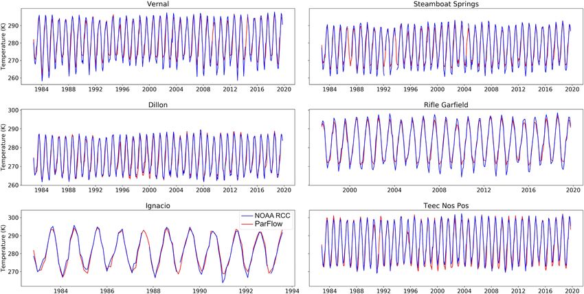
www.nature.com/scientificdata/                                                                     www.nature.com/scientificdata

                            Fig. 2 Plots of simulated and observed streamflow for eight gages within the UCRB. Streamflow predicted by
                            ParFlow is shown using the red line while streamflow predicted by the natural flow model is shown in blue.

                                The next observational set was the USGS groundwater database (https://waterdata.usgs.gov/nwis/gw). All
                            data from wells that have at least two months of observations during the period between 1983 and 2019 were
                            used for comparison here. Measurements that did not pass the USGS quality control (i.e. flagged for potential
                            measurement inconsistency or negative outlier values) were filtered out. Also, wells with water table depths
                            (WTD) below 52 m (i.e. below the depth for the center of the bottom grid cell in the model domain) were
                            removed. A total of 36 wells were used to compare water table levels after this filtering process (shown as blue
                            hexagons in Fig. 1).
                                In addition to these temporal groundwater observations, there are a total of 3,865 well locations in the UCRB
                            from the Fan et al.70 water table observations. Fan et al.70 compiled this water table observational dataset by
                            calculating the average WTD for USGS sites between 1927 and 2009. While Fan et al.70 noted that about 90%
                            of the wells have only one observation at different times, they found that wells whose WTD were above 20 m
                            aligned well with their global simulated WTD. Based on these findings, their dataset was determined to be an
                            appropriate resource to validate model performance.
                                We also employed a derived snow cover extent from MODIS for comparison to simulations. The daily
                            cloud-free snow cover dataset71 was developed via a series of mitigated cloud filters and the Variational
                            Interpolation algorithm to the MODIS-Snow Cover Area (SCA) Daily (MOD10C1 and MYD10C1) version
                            6 product12,72. The product has been proved to effectively capture the dynamic changes of snow from 2000 to
                            2017 with the average of Probability Of Detection and False Alarm Ratio are 0.955 and 0.179, respectively71. The
                            cloud-free product’s spatial and temporal resolutions are 0.05° and daily, respectively.
                                The Snow Water Equivalent (SWE) data was obtained from the Snow Telemetry (SNOTEL) network. There
                            was a total of 133 SNOTEL stations used for comparison. SNOTEL stations have an average elevation of nearly
                            2,900 m with the station in the highest elevation of more than 3,500 m at the Italian Creek, CO.
                                Total water storage (TWS) change measured by the Gravity Recovery and Climate Experiment (GRACE)
                            mission was used to compare with simulated TWS. Launched in 2002, GRACE estimates monthly changes
                            in terrestrial water storages globally based satellite location (http://www2.csr.utexas.edu/grace/RL05_mascons.
                            html). The data used in this study, CSR Release-06 GRACE Mascon Solutions, was released from the Center for
                            Space Research (CSR), the University of Texas at Austin. Mass fluxes (measured in terms of mass concentra-
                            tion—mascon) derived directly from raw GRACE data often have north-south stripes due to modeling errors,
                            measurement noise and observability issues73. To decrease the uncertainty in these mass fluxes, a series of filters
                            were applied to GRACE gravity information in a 1° geodesic grid domain. Those filters include (1) mascon geo-
                            desic grid correction, (2) Glacial Isostatic Adjustment (GIA) correction, (3) Degree-1 coefficients (Geocenter)
                            corrections and (4) C20 (degree 2 order 0) replacement. The final total water storage change is obtained by sub-
                            tracting the mean from 2003 to 2009. Please note that GRACE measures the storage anomaly at approximately
                            monthly intervals, but it does not measure total quantity of water stored. GRACE storage anomalies were avail-
                            able monthly from April 2002 to June 2017 at the time of this analysis with a spatial resolution of 1°. Given the
                            relatively low spatial resolution, Scalon et al.19 suggested to use GRACE only for watersheds which have areas
                            greater than 100,000 km2 (The area of the UCRB is approximately 280,000 km2). Uncertainty analysis for CSR
                            RL06 is not available yet, however, uncertainty value suggested for the RL05 version is roughly 2 cm73.
                                Four stations from the Community Collaborative Rain, Hail and Snow Network (CoCoRaHS) provide
                            potential ET estimates. Additionally, the AmeriFlux station at Niwot Ridge, CO (US-NR174,75) provides latent

Scientific Data |   (2022) 9:16 | https://doi.org/10.1038/s41597-022-01123-w                                                                 4
www.nature.com/scientificdata/                                                                               www.nature.com/scientificdata

                             Characteristic        Variables
                             Model outputs         Pressure; Saturation; CLM output
                             Data type             ParFlow Binary data
                             Data format           .pfb
                                                   ‘+proj = lcc +lat_1 = 30 +lat_2 = 60 +lat_0 = 40.00000762944445
                             Projection            +lon_0 = −97 +x_0 = 0 +y_0 = 0 +a = 6370000 +b = 6370000
                                                   +units = m +no_defs’
                             Spatial Coverage      −427000.645–468000.345; −1315000.309–708000.309
                             Spatial Resolution    1 km × 1 km
                             Temporal Coverage     October 1, 1982 to September 31, 2019
                             Temporal Resolution   1 hour

                            Table 1. Descriptive characteristics of the ParFlow output dataset.

                            heat observations (which can be translated directly to ET by dividing to a unit of latent heat of evaporation of
                            water 2256 kJ/kg). While ET stations are scarce in the UCRB, because of the diversity in their locations and
                            temporal coverage, we feel that those observations still play a crucial role in the simulation evaluation. First is
                            the range of elevation and land cover that those stations represent: two high elevation stations located at Niwot
                            Ridge, CO (3050 m) and Crested Butte, CO (2912 m), one moderate elevation station located at Carbondale, CO
                            (1887 m) and two low altitude stations located at Grand Junction, CO (1428 m) and Castle Valley, UT (1464 m).
                            With respect to land cover, stations at Carbondale, CO and Crested Butte, CO are located in evergreen forest;
                            stations at Niwot Ridge, CO and Grand Junction, CO are located in deciduous forest; the station at Castle Valley,
                            UT is located in shrubland. We compared ParFlow simulations with CoCoRaHs data from June 2012 to present
                            and AmeriFlux data from 1999 to present, respectively.
                                In addition to ET estimated from stations, we also used remotely sensed ET from Simplified Energy Balance
                            (SSEBop) MODIS product to compare with simulated ET. The SSEBop model provides daily and 1-km ET esti-
                            mations for the whole UCRB from 2000 to the end of the validation period and has been shown to be reliable in
                            various regions76,77. Senay et al.78 simulates ET in SSEBop by using pre-defined hot and cold boundary condi-
                            tions. Each pixel is assigned a hot and cold boundary values based on maximum air temperature and differential
                            temperature. Based on land surface temperature (K) obtained from MODIS images, ET fraction is computed
                            and then multiplied with a short grass reference (mm.d−1) and a scaling coefficient to produce final ET79.
                                Lastly, ground temperature data from the National Oceanic and Atmospheric Administration (NOAA)
                            Regional Climate Center (RCC) was used for comparison. The NOAA RCC data consist of observations com-
                            piled from the Global Historical Climatology Network (GHCN80) database, and other federal and regional agen-
                            cies. There are a total of 490 stations that monitor temperature. These stations are well distributed over the UCRB
                            (green diamonds in Fig. 1).
                                Two of the remotely sensed products used for comparison, namely, MODIS-SCA and GRACE, are down-
                            scaled to match with the dataset’s spatial resolution of 1-km and geographic projection (specified at Table 1).
                            Specifically, MODIS-SCA and GRACE data were downscaled from 5-km and 100-km, respectively, to 1-km
                            using the Nearest Neighbor algorithm.

                            Evaluation metrics.         For timeseries data, we primarily used two metrics to evaluate model performance,
                            Spearman’s Rho and Total Absolute Relative Bias. As explained in Maxwell and Condon38, plotting these two met-
                            rics against one another produces a figure that will concisely describe a model’s ability to reproduce appropriate
                            timing and magnitude of flows. We hereafter refer to this type of figure as a Condon Diagram. Spearman’s Rho
                            was used to assess the differences in the simulated and observed variables timing while the relative bias measures
                            differences in their volumes. If simulations are closed to observation, we expect high Speaman’s Rho value and
                            low relative bias value. Spearman’s Rho is computed as:

                                                                                              6∑ ni =1d i2
                                                                            srho = 1 −
                                                                                             n(n 2 − 1)                                     (1)
                            where di is the difference in the independent ranking for the simulated and observed values at i time step, n is the
                            number of values in each time series. The Total Absolute Relative Bias is calculated as:
                                                                                        n           n
                                                                                      ∑ i =1Si − ∑ i =1Oi
                                                                         bias =                n
                                                                                            ∑ i =1Oi                                        (2)
                            where S and O are simulated and observed timeseries, respectively, and n is the number of values in each time
                            series.
                                Additionally, we used the Kling-Gupta Efficiency (KGE81,82) to evaluate the streamflow performance. The
                            KGE coefficient is proposed by Gupta et al.81 to achieve a more balanced evaluation of simulated mean flow, flow
                            variability and daily correlation than the traditional Nash-Sutcliffe efficiency (NSE83)84,85.
                                For spatial data, we used two categorical validation indices, namely, Probability of Detection and False Alarm
                            Ratio:

Scientific Data |   (2022) 9:16 | https://doi.org/10.1038/s41597-022-01123-w                                                                  5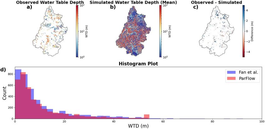
www.nature.com/scientificdata/                                                                                       www.nature.com/scientificdata

                             Variable                           Abbreviation      Unit      Spatial resolution
                             Visible or short-wave radiation    DSWR              W/m2      1 km
                             Long wave radiation                DLWR              W/m2      1 km
                             Precipitation                      APCP              mm/s      1 km
                             Air Temperature                    Temp              K         1 km
                             East-West wind speed               UGRD              m/s       1 km
                             South-North wind speed             VGRD              m/s       1 km
                             Atmospheric pressure               Press             pa        1 km
                             Specific humidity                  SPFH              kg/kg     1 km

                            Table 2. Hourly NLDAS inputs for the simulation.

                             File                                       Description
                             UpperCO.slope[x/y].rivth1500.pfb           Topographic slopes in x and y directions
                             UpperCO_init_press_1982.pfb                Initial pressure after the spin up process
                             UpperCO_IndicatorFile_v2.pfb               3-D indicator file of different soil, geology and bedrock types
                             UpperCO_v2.pfsol                           3-D solid file of the model domain
                             Drv_clmin_v2.dat                           Parameters of CLM model
                             Drv_vegm_v2.UC.dat                         Vegetation type, cartesian coordinates for each grid of the domain
                             Drv_vegp.dat                               Vegetation parameters for the IGBP classification

                            Table 3. Files that contain the model input parameters for the simulation.

                                                                                                   Hit
                                                                                  POD =
                                                                                               Hit + Miss                                       (3)

                                                                                                  False
                                                                                  FAR =
                                                                                               Hit + False                                      (4)
                            where Hit is grid where both simulated and observed events occurred; Miss is grid cell where the observed event
                            occurred but the simulated one did not; False is a grid cell where the simulated event occurred but the observed
                            one did not.

                            Data Records
                            The dataset is available to the public through an unrestricted data repository hosted by CyVerse86. All the
                            inputs for the simulation are included, namely, NLDAS (Table 2), related hydrologic and land-surface variables
                            (Table 3) and a TCL script that contains the complete list of ParFlow input keys for the simulation.
                                For each WY of simulation time, there are three output files per hourly timestep, namely, pressure, saturation
                            and CLM output.
                                The hourly outputs shown in Table 4 and inputs shown in Table 2 were averaged into monthly variables for
                            comparison to observations. Some additional quantities were calculated from ParFlow outputs (e.g. water table
                            depth). These variables are listed in Table 5.
                                ParFlow grid data is stored in a ParFlow binary file format (.pfb) which is written as BIG ENDIAN binary
                            bit ordering. More information about ParFlow binary file format can be found in the ParFlow manual (https://
                            github.com/parflow/parflow/blob/master/parflow-manual.pdf). Developed modules that read the ParFlow
                            binary files can be found at https://github.com/parflow/parflow/tree/master/pftools/prepostproc and https://
                            github.com/hydroframe/parflowio.
                            Technical Validation
                            In this section we compared simulated water and energy fluxes to a wide range of datasets for the UCRB from
                            1983 to 2019, including station measurements and modeled outputs to validate the fidelity of the simulation and
                            prioritize for future model improvement. The available station measurements were streamflow, water table depth
                            (WTD), snowpack, water storage and evapotranspiration (Fig. 1). The available modeled outputs were Snow
                            Cover Area, Total Water Storage Anomalies, and evapotranspiration.

                            Streamflow comparisons. We compared simulated and observed monthly streamflow for eight represent-
                            ative stations within the UCRB (Fig. 2). Streamflow varied over two orders of magnitude with peak flow from
                            around 2000 (ft3/s) at East River at Almont station to around 40,000 (ft3/s) at Colorado River near Cisco station
                            and at Green River at Green River station. Simulated streamflow reflected accurately wet (1983–1985, 1993–1996,
                            2008–2010) and dry (1989–1992, 2002–2004, 2011–2013,2018) periods. In general, simulated flows matched
                            observed ones well with average relative bias and Spearman’s Rho of 0.15 and 0.51, respectively.

Scientific Data |   (2022) 9:16 | https://doi.org/10.1038/s41597-022-01123-w                                                                         6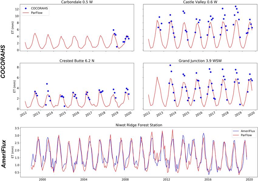
www.nature.com/scientificdata/                                                                                      www.nature.com/scientificdata

                             Variable                                                      Unit         Files
                             Pressure Head at every grid cell (3D)                         [m]          ParFlow Pressure
                             Saturation at every grid cell (3D)                            [m3/m3]      ParFlow Saturation
                             total latent heat flux                                        [W/m2]       CLM layer 0
                             total upward LW radiation                                     [W/m2]       CLM layer 1
                             total sensible heat flux                                      [W/m2]       CLM layer 2
                             ground heat flux                                              [W/m2]       CLM layer 3
                             net veg. evaporation and transpiration and soil evaporation   [mm/s]       CLM layer 4
                             ground evaporation                                            [mm/s]       CLM layer 5
                             soil evaporation                                              [mm/s]       CLM layer 6
                             vegetation evaporation (canopy) and transpiration             [mm/s]       CLM layer 7
                             transpiration                                                 [mm/s]       CLM layer 8
                             infiltration flux                                             [mm/s]       CLM layer 9
                             SWE                                                           [mm]         CLM layer 10
                             ground temperature                                            [K]          CLM layer 11
                             irrigation flux                                               [na]         CLM layer 12
                             Soil temperature layer 1                                      [K]          CLM layer 13
                             Soil temperature layer 2                                      [K]          CLM layer 14
                             Soil temperature layer 3                                      [K]          CLM layer 15
                             Soil temperature layer 4                                      [K]          CLM layer 16

                            Table 4. Hourly ParFlow-CLM output variables and units.

                             Variables                    Unit            Source
                             Water Ponding Depth          m               ParFlow Pressure output
                             Water Table Depth            m               ParFlow Pressure output
                             Snow Water Equivalent        mm/month        ParFlow CLM output
                             Total Water Storage          mm/month        ParFlow Pressure and Saturation output
                             Evapotranspiration           mm/day          ParFlow CLM output
                             Ground Temperature           K               ParFlow CLM output
                             Precipitation                mm/day          NLDAS Input
                             Soil Moisture                —               ParFlow Saturation output and static Porosity Input

                            Table 5. Monthly variables derived from the ParFlow output/input datasets.

                                The simulated and observed streamflow were in good agreement at Colorado River near Cisco station and
                            at Green River at Green River station with low relative bias of 0.4 and 0.35 and high Spearman’s Rho of 0.52 and
                            0.73, respectively. Simulated flows at stations from the San Juan River had moderate bias between 1989 and 1992,
                            but the bias reduced later. In the drought years between 1989 and 1992, we found NLDAS indicated more snow
                            than one measured from SNOTEL and snow melt later than from SNOTEL, this snow component in NLDAS
                            caused the moderate bias in streamflow simulation.
                                We found some discrepancies between streamflow simulations and observations in the station San Juan River
                            near Bluff which could be attributed to anthropogenic activities. Model results were also compared to the Bureau
                            of Reclamation natural flow dataset. Figure 3 shows examples of streamflow performances for two stations that
                            are affected by upstream dams: San Juan River near Bluff and Colorado River at Lees Ferry. Overall, the ParFlow
                            results shown in Fig. 3 are in good agreement with the naturalized flows. In the Colorado River at Lees Ferry sta-
                            tion, the natural flow and ParFlow showed similar peaks and low streamflow bias across the comparison period.
                            The mean monthly hydrograph comparisons highlighted a good correlation in seasonal cycles between the
                            ParFlow results and the naturalized flows (Fig. 3). However, the ParFlow results were lower than the naturalized
                            flows during summer and early winter in both stations (Fig. 3).
                                Streamflow performance using Spearman’s Rho and relative bias is shown in Fig. 4 for all stations inside the
                            UCRB. Stations were considered to have a good shape (i.e. matching temporal pattern) when their Spearman’s
                            Rho values are greater than 0.5 and bad shape when their Spearman’s Rho values were smaller than 0.5. Likewise,
                            stations were considered as low bias if their relative biases were smaller than 1 and high bias if their relative
                            biases were greater than 1. Hence, there were four types of streamflow performance: (1) stations with good shape
                            and low bias – green stations; (2) stations with good shape and high bias – blue stations; (3) stations with bad
                            shape and low bias – purple stations; (4) stations with bad shape and high bias – red stations.
                                Despite the complex terrain of the UCRB, most of the stations (94%) had relative bias lower than 1. The
                            majority of stations (52%) had both low bias and good shape (i.e. relative bias smaller than 1 and Spearman’s Rho
                            greater than 0.5), most of them located in the upstream part of rivers originating from the Rocky Mountains,
                            namely, the Gunnison, Yampa and San Juan. Simulated flows matched with observed ones along the Green River

Scientific Data |   (2022) 9:16 | https://doi.org/10.1038/s41597-022-01123-w                                                                        7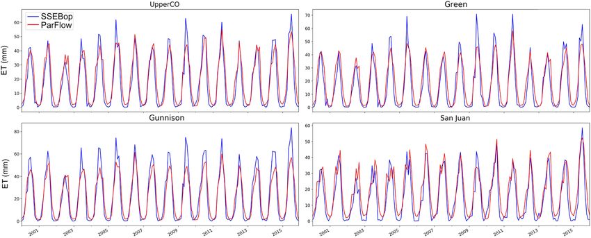
www.nature.com/scientificdata/                                                                     www.nature.com/scientificdata

                            Fig. 3 Natural flow comparison for two stations that are affected by upstream dams: San Juan River near Bluff
                            and Colorado River at Lees Ferry. Streamflow predicted by ParFlow is shown using the red line while streamflow
                            predicted by the natural flow model is shown in blue. Two panels above indicate monthly streamflow and two
                            panels bellow indicate mean monthly for each month during the simulation period.

                            Fig. 4 (a) The Condon-diagram streamflow performance plot, (b) the performance category of each gage
                            within the UCRB domain.

                            (Figs. 2 and 4). Stations with bad shape generally fall into two categories: (1) impacted by anthropogenic activ-
                            ities (e.g. stations along the Colorado River); (2) located in relatively small streams (e.g. western tributaries of
                            the Green River or tributaries of the San Juan River). The results agreed well with previous ParFlow streamflow
                            evaluations of the UCRB38,87.

                            Water table depth comparisons.                 A representative sample of wells is taken for comparison between
                            observed and simulated WTD (Fig. 5). ParFlow-CLM accurately simulated both timing and magnitude for most
                            of the wells, however there were some points of discrepancy.
                                Overall, both streambank and deep wells had good agreements between simulations and observations with
                            the relative bias for 14 wells out of 24 wells was smaller than 0.3. Simulated WTDs at the Lower Gunnison River
                            Basin (LGRB) matched close to observations in mean depth and temporal variability. Similarly, simulated stre-
                            ambank wells (e.g. at station 09205000 (left) and at station 09209400 (left and right) showed a good agreement
                            with observed WTD. An exception to this close agreement was the well at the right bank of station 09205000
                            where simulated WTD showed much greater seasonal cycles than observed.

Scientific Data |   (2022) 9:16 | https://doi.org/10.1038/s41597-022-01123-w                                                                  8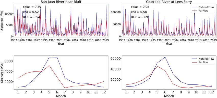
www.nature.com/scientificdata/                                                                   www.nature.com/scientificdata

                            Fig. 5 Time series plots of predicted and observed water table depths for available USGS wells within the basin.

                                Deep wells with WTD of around 20 m such as 19–105-10bbb01 Rock Springs (near Rock Springs, WY)
                            and (D-36-22)22daa-1 (near Blanding, UT), showed decreasing and increasing trends, respectively, over time
                            and simulated WTD shows similar trends. With wells that are close to the maximum WTD of the domain (e.g.
                            (D-33-24)30dab-1), simulated WTD did not reflect the observed multi-year cycle in these locations. This bias
                            was likely caused by the model spatial resolution. Deeper wells are often located in mountainous areas where the
                            topography is complex. ParFlow-CLM’s 1-km resolution may not be sufficient to capture this type of behavior.
                            Please note that all wells were mapped to the closest grid cell center with no further adjustment.
                                We also compared the average simulated WTD (Fig. 6b) with the average USGS WTD dataset compiled
                            from Fan et al. 2013 (Fig. 6a). Most of the wells had WTD differences of less than 1 m compared to the simu-
                            lations, and some deep wells (around 40-m depth) in the Green and San Juan sub basins were 2–4 m deeper
                            than the simulated. The observed dataset had more shallow water tables than simulated (Fig. 6c,d) and sim-
                            ulated WTD had more points which reach the maximum depth of 52-m (Fig. 6d). The output WTD was on
                            average over one square kilometer (model grid spatial resolution). Most of the “max depth” points were in
                            the mountainous areas where the average output WTD was often dominated by WTD that is close to 52-m.
                            This often led to overestimation of the depth (i.e. WTDs are deeper than in observation wells). However, the
                            WTD average for most of the well was consistent with the observations with nearly 2,650 wells (70%) having
                            absolute differences smaller than 0.5 m. Lastly, the average of absolute difference in depth for all the wells
                            was 1.042 m.

                            Snow covered extent comparison. We compared the simulated SCA to one obtained from the cloud-free
                            MODIS product (Fig. 7a). Model outputs were upscaled and averaged to match with the cloud-free product’s
                            spatial and temporal resolutions. Simulated SCA had consistent high Probability of Detection (average 0.82)
                            throughout the period of 17 year (Fig. 7b). False Alarm Ratio was often high (around 0.4) during accumulating
                            and melting months (i.e. October and April, respectively). During winter, simulated SCA accurately reflected the
                            dynamic of SCA with almost 100% snow pixel captured and below 5% overestimated snow pixels. For typically
                            dry years such as 2001, 2002 and 2016, ParFlow-CLM tended to produce slightly more SCA.
                                Figure 7c shows a snapshot of comparison between simulated and cloud-free MODIS SCA in a melting
                            month of April 2008. Both SCAs agreed well in the Green and Gunnison river basins. Cloud-free MODIS SCA
                            indicated that snow had already melted in various places along the Colorado River and Northern Arizona (lower
                            left of the UCRB) while it was contrasting in the simulated SCA. Lastly, the model missed some snowpack in
                            Northern New Mexico (lower right of the UCRB). A detailed discussion regarding sources of bias in snow sim-
                            ulation is covered in the next section.
                            Snow water equivalent comparisons. All SWE stations were mapped to the closest grid cell center with
                            no adjustments made to scale point value to grid block or to adjust for differences between the station’s eleva-
                            tion and the mean grid cell elevations. Comparison results for six representative stations from Green, Gunnison
                            and San Juan basins are shown in Fig. 8. While Rock Creek and Strawberry Divide stations are in Green basin,
                            Summit Ranch and Butte stations are in Gunnison basin, Cascade and Mineral Creek are in San Juan basin
                            (Fig. 9). Elevations of these stations ranges from the lowest of 2403 m (Rock Creek) to the highest of 3100 m
                            (Butte). In general, simulated and observed SWE agreed on peak timing and magnitude trend over the period.

Scientific Data |   (2022) 9:16 | https://doi.org/10.1038/s41597-022-01123-w                                                               9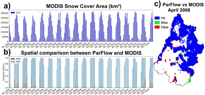
www.nature.com/scientificdata/                                                                  www.nature.com/scientificdata

                            Fig. 6 Spatial comparisons of water table depth averaged over the entire simulation. (a) Average WTD for
                            USGS sites between 1927 and 2009 from Fan et al. (2013), (b) The average WTD from this simulation, (c)
                            observed-simulated WTD, (d) histogram of simulated and observed WTD.

                            Fig. 7 (a) MODIS monthly snow cover area (SCA) for the Upper Colorado River Basin from 2000 to 2016.
                            (b) Spatial comparison between ParFlow and MODIS SCA using two categorical validations, namely,
                            Probability of Detection and False Alarm Ratio. (c) An example of spatial comparison between ParFlow SCA
                            and MODIS SCA.

                            Simulated SWE accurately reflected drought periods (i.e. 1988–1990, 2002–2004, 2012–2014 and 2018) and wet
                            periods (1983–1985, 1993–1995 and 2008–2010).
                                However, before 2003, simulated SWE was systematically lower than observed in all stations. This dry bias
                            was worst in the Strawberry Divide station, where simulated peak monthly SWE was often 200 mm lower than
                            the observed. A potential source of bias was directly linked to the NLDAS dataset. Earlier version of NLDAS
                            used in this simulation from WY 1983 to WY 2002 has been shown to have SWE bias from: (1) dry bias in
                            annual precipitation, (2) air temperatures are systematically lower in winter and higher in spring, (3) coarse
                            spatial resolution of 1/8° 49,50. For simulation from WY 2003, we used a newer version of NLDAS which was
                            greatly enhanced in precipitation and temperature estimations88. The dry SWE bias was much alleviated overall
                            although the bias persisted during some drought years of 2012 and 2013.

Scientific Data |   (2022) 9:16 | https://doi.org/10.1038/s41597-022-01123-w                                                           10
www.nature.com/scientificdata/ www.nature.com/scientificdata
Fig. 8 Time series plots of predicted and observed (SNOTEL) SWE over the simulation time period for six
SNOTEL stations within the UCRB.
Fig. 9 (a) Predicted-observed bias for all the SNOTEL stations within the UCRB, and (b) plot of the fraction of
SNOTEL stations with snow compared to the equivalent model simulated output.
Figure 9 shows an interesting contradiction. While simulated maximum annual SWE was lower than
observed SWE for most of the stations (Fig. 9a), when doing monthly average by year, ParFlow-CLM simu-
lated earlier snow accumulation and later snow melt than observations (Fig. 9b). In the Green basin, maxi-
mum annual SWEs were often lower by 100 m than observations. In contrast, basins in higher altitude such as
Gunnison and San Juan had both underestimated (smaller by 200 mm) and overestimated (greater by 100 mm)
stations.
Beside bias in forcing, there always existed an inconsistency when comparing point measurements with
the model 1-km grid. The model grid resolution could smooth out the dynamic changes of snowpack in high
altitude regions. Figure 9b shows a reverse pattern of fraction of station with snow between SNOTEL and
ParFlow-CLM that Maxwell and Condon (2016) found in water year 1985. The reverse pattern could be a result
of replacing forcing inputs in the second half of the decadal simulation.
GRACE terrestrial water storage comparison. Changes in water storage from GRACE were com-
pared with the ParFlow-CLM simulation from 2002 and 2017 (Fig. 10). Water storage change from GRACE
was obtained by subtracting the water storage mean from 2004 to 2009. We also did the same process with out-
puts from ParFlow-CLM to ensure the consistency in comparison. Thus, we compared between the products
basin-wide.
Two products agreed well from 2003 to 2011. Drought years of 2003 and 2004 were accurately reflected as
well as wet years of 2005, 2008 and 2011. During periods of data discrepancy from GRACE (i.e. 2002 and from
2011 to 2017), GRACE showed much lower water storage anomaly than ParFlow-CLM.
Scientific Data | (2022) 9:16 | https://doi.org/10.1038/s41597-022-01123-w 11www.nature.com/scientificdata/ www.nature.com/scientificdata
Fig. 10 Time series plot of the total water storage anomaly from the model simulations and the GRACE
estimates.
ET comparisons. Direct observations of ET and/or latent heat were from two sources: (1) AmeriFlux
network (one station, data from 1999) and (2) COCORAHS (four stations, data from 2012). Stations from
COCORAHS measure potential evaporation. Measuring potential ET rather than actual ET by COCORAHS
explained the systematic underestimation of simulated ET in months of June and July for Grand Junction and
Crested Butte and in months of May, June and July for Castle Valley, as potential ET would be greater than actual
ET. For other summer months, ParFlow-CLM simulated accurately with observations (Fig. 11).
The Niwot Ridge Forest station from the AmeriFlux network is located at 3050 m elevation in subalpine
forest. Flux magnitude and trend from both simulated and observed ET were overall matching (Fig. 11). Niwot
Ridge station showed small amounts of evaporation (around 1.5 mm) during winters of 1999, 2000, 2007, 2009
and 2014 while ParFlow-CLM did not show winter ET values.
When comparing with a remotely sensed product (SSEBop) over the entire basin, the simulated ET had
lower ET peak than SSEBop in the Green, Gunnison and ultimately Upper Colorado River basins (Fig. 12).
In the San Juan basin, the two ET estimates agreed well over the period. The SSEBop’s estimation approach is
fundamentally different from the physical based modelling of ParFlow-CLM, and thus requires detailed com-
parisons of model specifications in order to examine the difference in ET.
Land surface temperature comparison. Simulated and observed ground temperature matched closely
throughout the study period. Out of 490 NOAA RCC stations, 263 stations had Spearman’s Rho value greater than
0.95, 486 stations had relative bias smaller than 0.05. Figure 13 shows comparison for six representative stations
for the Green, Gunnison and San Juan basins (Vernal and Steamboat Springs in Green, Dillon and Rifle Garfield
in Gunnison, Ignacio and Teec Nos Pos in San Juan). We can see great matches between simulations and observa-
tions in different terrains and temperature ranges.
Comparison summary. We compared seven variables output from the decadal simulation, (1) streamflow,
(2) water table depth, (3) snow cover area, (4) snow water equivalent, (5) actual evapotranspiration, (6) total stor-
age water anomalies and (7) ground temperature, to observations and data products. In general, this comparison
demonstrates good agreements between model and observations and data products.
A summary of comparisons is given in Tables 6, 7. The average relative bias for streamflow, WTD, SWE,
ET and temperature was 0.123. For this pre-development simulation, more than half of the stream gauges
(53%) had good timing correlation (Spearman’s Rho > 0.5) between simulated and observed streamflow. This
simulation accurately captured the mean WTD with 70% of the wells having absolute difference in mean
WTD smaller than 0.5 m. Other land surface variables such as: SWE, ET, TWSA and ground temperature also
showed a good match to observations and had an average relative bias of 0.078 and an average Spearman’s Rho
of 0.838.
Sources of bias in simulated streamflow and WTD were due to four reasons: (1) lateral and vertical resolu-
tions; (2) water management operations; (3) bias in meteorological forcing data; (4) uncertainties in subsurface
properties.
Usage Notes
In the CyVerse repository, beside ParFlow output files, we also provided necessary input files to reproduce the
simulation. Specifically, we included (1) NLDAS data; (2) ParFlow and CLM parameter files (e.g. vegetation
parameter file, subsurface indicator file and topographic information files); (3) A tcl script for running the sim-
ulation. More information can be found in the repository readme file.
Interested users are encouraged to use the newly developed parflowio tool (https://github.com/hydroframe/
parflowio) to work with.pfb format files.
While it was shown that anthropogenic activities reflected in USGS streamflow and WTD still contributed
to the comparison bias, the results are encouraging with most of the gauges and wells having low relative bias
and high Spearman’s Rho scores. As Maxwell and Condon38 indicated that the ParFlow simulation platform
Scientific Data | (2022) 9:16 | https://doi.org/10.1038/s41597-022-01123-w 12www.nature.com/scientificdata/ www.nature.com/scientificdata
Fig. 11 Comparison between simulated ET and estimates of ET based on observations. The upper four panels
are potential evaporation from the COCORAHS network, the bottom panel actual ET from the Niwot Ridge
eddy covariance station.
Fig. 12 Comparisons between the SSEBop remote sensing product and model simulations for ET for the entire
domain (UpperCO) and three major sub-basins.
is evolving with more refined surface89 and subsurface and more anthropogenic activities coupled, the model
formulation will be improved.
The dataset produced in this study is useful in hydrological studies due to its high spatial and temporal reso-
lutions and validated accuracy. Moreover, having more consistent data about the groundwater dynamic, one can
study its impact on the full water cycle of the UCRB and possibly other river basins. We hope the dataset will be
used for a wide range of stakeholders from decision makers to ecologic scientists.
Scientific Data | (2022) 9:16 | https://doi.org/10.1038/s41597-022-01123-w 13www.nature.com/scientificdata/ www.nature.com/scientificdata
Fig. 13 Land surface temperature comparison plots for model simulations and observations at six stations
within the UCRB.
Variable Measured Average Monthly Average Monthly Average Depth Number of
Point Observation (unit) Relative Bias Spearman’s Rho Difference Stations
USGS stream gauges Discharge (ft3/s) 0.043 0.460 — 602
Bureau of Reclamation’s natural flow Discharge (ft3/s) 0.05 0.68 20
USGS wells WTD (m) 0.356 0.432 — 36
Fan et al. Compile WTD WTD (m) — — 1.042 3865
SNOTEL SWE (mm) 0.213 0.840 — 133
CoCoRaHS Potential ET (mm/d) 0.123 0.667 — 4
AmeriFlux Actual ET (mm/d) 0.001 0.854 — 1
NOAA RCC Temperature (K) 0.001 0.958 — 490
Table 6. Comparison summary for point observations.
Remotely sensed Variable Temporal Average Monthly Average Monthly Average Average Monthly
Product Measured (unit) Coverage Relative Bias Spearman’s Rho Monthly POD FAR
Cloud-free March 2000–
SCA (km2) — — 0.737 0.193
MODIS SCA February 2017
Actual ET March 2000–
MODIS SSEBop 0.050 0.866 — —
(mm/month) December 2015
CSR GRACE Total water storage April 2002–
0.069 0.863 — —
RL06 Mascon change (mm) June 2017
Table 7. Comparison summary for remotely sensed products.
Code availability
These simulations were conducted using ParFlow version 3.6.0 (https://github.com/parflow/parflow/tree/v3.6.0/).
The data processing step was done using Python3.5 programming language with necessary toolboxes including
NumPy (https://numpy.org/), the Geospatial Data Abstraction Library (GDAL; https://gdal.org/) and the Python
Data Analysis Library (PANDAS; https://pandas.pydata.org/).
Received: 6 January 2021; Accepted: 10 December 2021;
Published: xx xx xxxx
References
1. Christensen, N. S., Wood, A. W., Voisin, N., Lettenmaier, D. P. & Palmer, R. N. The effects of climate change on the hydrology and
water resources of the Colorado River basin. Clim. Change 62, 337–363 (2004).
2. Christensen, N. S. & Lettenmaier, D. P. A multimodel ensemble approach to assessment of climate change impacts on the hydrology
and water resources of the Colorado River Basin. Hydrol. Earth Syst. Sci. 11, 1417–1434 (2007).
Scientific Data | (2022) 9:16 | https://doi.org/10.1038/s41597-022-01123-w 14www.nature.com/scientificdata/ www.nature.com/scientificdata
3. McCabe, G. J. & Wolock, D. M. Warming may create substantial water supply shortages in the Colorado River basin. Geophys. Res.
Lett. 34 (2007).
4. Milly, P. C. D. & Dunne, K. A. Colorado River flow dwindles as warming-driven loss of reflective snow energizes evaporation. Science
(80-.). 367, 1252–1255 (2020).
5. Ficklin, D. L., Stewart, I. T. & Maurer, E. P. Climate change impacts on streamflow and subbasin-scale hydrology in the Upper
Colorado River Basin. PLoS One 8 (2013).
6. Overpeck, J. T. & Udall, B. Climate change and the aridification of North America. Proceedings of the National Academy of Sciences
of the United States of America. 117, 11856–11858 (2020).
7. National Research Council. Colorado River Ecology and Dam Management: Proceedings of a Symposium, May 24–25, 1990 Santa Fe,
New Mexico. (1991).
8. Belnap, J. & Campbell, D. Effects of climate change and land use on water resources in the Upper Colorado River Basin. https://doi.
org/10.3133/fs20103123 (2011).
9. Andersen, D. C., Cooper, D. J. & Northcott, K. Dams, floodplain land use, and riparian forest conservation in the semiarid Upper
Colorado River Basin, USA. Environ. Manage. 40, 453–475 (2007).
10. DeWine, J. M. & Cooper, D. J. Effects of river regulation on riparian box elder (Acer negundo) forests in canyons of the upper
Colorado River Basin, USA. Wetlands 27, 278–289 (2007).
11. Woodhouse, C. A., Gray, S. T. & Meko, D. M. Updated streamflow reconstructions for the Upper Colorado River Basin. Water
Resour. Res. 42 (2006).
12. Hall, D. K., Riggs, G. A., Salomonson, V. V., DiGirolamo, N. E. & Bayr, K. J. MODIS snow-cover products. Remote Sens. Environ. 83,
181–194 (2002).
13. Maurer, E. P., Rhoads, J. D., Dubayah, R. O. & Lettenmaier, D. P. Evaluation of the snow-covered area data product from MODIS.
Hydrol. Process. 17, 59–71 (2003).
14. Policelli, F. et al. The NASA Global Flood Mapping System. in 47–63, https://doi.org/10.1007/978-3-319-43744-6_3 (2017).
15. Tran, H. et al. Improving hydrologic modeling using cloud-free modis flood maps. J. Hydrometeorol. 20, 2203–2214 (2019).
16. Gu, Y. et al. Evaluation of MODIS NDVI and NDWI for vegetation drought monitoring using Oklahoma Mesonet soil moisture
data. Geophys. Res. Lett. 35 (2008).
17. Caccamo, G., Chisholm, L. A., Bradstock, R. A. & Puotinen, M. L. Assessing the sensitivity of MODIS to monitor drought in high
biomass ecosystems. Remote Sens. Environ. 115, 2626–2639 (2011).
18. Rodell, M. et al. Emerging trends in global freshwater availability. Nature 557, 651–659 (2018).
19. Scanlon, B. R. et al. Global evaluation of new GRACE mascon products for hydrologic applications. Water Resour. Res. 52,
9412–9429 (2016).
20. Koster, R. D. & Suarez, M. J. Modeling the land surface boundary in climate models as a composite of independent vegetation stands.
J. Geophys. Res. 97, 2697–2715 (1992).
21. Koster, R. D. & Suarez, M. J. The components of a ‘SVAT’ scheme and their effects on a GCM’s hydrological cycle. Adv. Water Resour.
17, 61–78 (1994).
22. Chen, F. et al. Modeling of land surface evaporation by four schemes and comparison with FIFE observations. J. Geophys. Res. Atmos.
101, 7251–7268 (1996).
23. Koren, V. et al. A parameterization of snowpack and frozen ground intended for NCEP weather and climate models. J. Geophys. Res.
Atmos. 104, 19569–19585 (1999).
24. Burnash, R., Ferral, R. & McGuire, R. A generalized streamflow simulation system - Conceptual modeling for digital computers. (U.S.
Department of Commerce, 1973).
25. Anderson, E. A. National Weather Service River Forecast System - Snow Accumulation and Ablation Model. NOAA Technical
Memorandum NWS HYDRO-17. NOAA Technical Memorandum NWS HYDRO-17, 1–87 (1973).
26. Liang, X., Lettenmaier, D. P., Wood, E. F. & Burges, S. J. A simple hydrologically based model of land surface water and energy fluxes
for general circulation models. J. Geophys. Res. 99 (1994).
27. Wood, E. F., Lettenmaier, D., Liang, X., Nijssen, B. & Wetzel, S. W. Hydrological modeling of continental-scale basins. Annu. Rev.
Earth Planet. Sci. 25, 279–300 (1997).
28. Painter, T. H., Skiles, S. M. K., Deems, J. S., Bryant, A. C. & Landry, C. C. Dust radiative forcing in snow of the Upper Colorado River
Basin: 1. A 6 year record of energy balance, radiation, and dust concentrations. Water Resour. Res. 48 (2012).
29. Liu, Y., Peters-Lidard, C. D., Kumar, S. V., Arsenault, K. R. & Mocko, D. M. Blending satellite-based snow depth products with in situ
observations for streamflow predictions in the Upper Colorado River Basin. Water Resour. Res. 51, 1182–1202 (2015).
30. Maxwell, R. M. & Miller, N. L. Development of a coupled land surface and groundwater model. J. Hydrometeorol. 6, 233–247 (2005).
31. Kollet, S. J. & Maxwell, R. M. Integrated surface-groundwater flow modeling: A free-surface overland flow boundary condition in a
parallel groundwater flow model. Adv. Water Resour. 29, 945–958 (2006).
32. Maxwell, R. M. A terrain-following grid transform and preconditioner for parallel, large-scale, integrated hydrologic modeling. Adv.
Water Resour. 53, 109–117 (2013).
33. Richards, L. A. Capillary conduction of liquids through porous mediums. J. Appl. Phys. 1, 318–333 (1931).
34. Kollet, S. J. & Maxwell, R. M. Capturing the influence of groundwater dynamics on land surface processes using an integrated,
distributed watershed model. Water Resour. Res. 44 (2008).
35. Kollet, S. J. et al. The Influence of Rain Sensible Heat and Subsurface Energy Transport on the Energy Balance at the Land Surface.
Vadose Zo. J. 8, 846–857 (2009).
36. Maxwell, R. M., Condon, L. E. & Kollet, S. J. A high-resolution simulation of groundwater and surface water over most of the
continental US with the integrated hydrologic model ParFlow v3. Geosci. Model Dev. 8, 923–937 (2015).
37. Jefferson, J. L. & Maxwell, R. M. Evaluation of simple to complex parameterizations of bare ground evaporation. J. Adv. Model. Earth
Syst. 7, 1075–1092 (2015).
38. Maxwell, R. M. & Condon, L. E. Connections between groundwater flow and transpiration partitioning. Science (80-.). 353, 377–380
(2016).
39. Kuffour, B. N. O. et al. Simulating coupled surface-subsurface flows with ParFlow v3.5.0: Capabilities, applications, and ongoing
development of an open-source, massively parallel, integrated hydrologic model. Geosci. Model Dev. 13, 1373–1397 (2020).
40. Horton, R. E. The Rôle of infiltration in the hydrologic cycle. Eos, Trans. Am. Geophys. Union 14, 446–460 (1933).
41. Dunne, T. Relation of field studies and modeling in the prediction of storm runoff. J. Hydrol. 65, 25–48 (1983).
42. Ryken, A., Bearup, L. A., Jefferson, J. L., Constantine, P. & Maxwell, R. M. Sensitivity and model reduction of simulated snow
processes: Contrasting observational and parameter uncertainty to improve prediction. Adv. Water Resour. 135 (2020).
43. Dai, Y. et al. The common land model. Bull. Am. Meteorol. Soc. 84, 1013–1023 (2003).
44. Condon, L. E. & Maxwell, R. M. Systematic shifts in Budyko relationships caused by groundwater storage changes. Hydrol. Earth
Syst. Sci. 21, 1117–1135 (2017).
45. Xia, Y. et al. Continental-scale water and energy flux analysis and validation for the North American Land Data Assimilation System
project phase 2 (NLDAS-2): 1. Intercomparison and application of model products. J. Geophys. Res. Atmos. 117 (2012).
46. Lohmann, D. et al. Streamflow and water balance intercomparisons of four land surface models in the North American Land Data
Assimilation System project. J. Geophys. Res. Atmos. 109 (2004).
Scientific Data | (2022) 9:16 | https://doi.org/10.1038/s41597-022-01123-w 15You can also read