When Nudges Fail to Scale: Field Experimental Evidence from Goal Setting on Mobile Phones
←
→
Page content transcription
If your browser does not render page correctly, please read the page content below

// NO.20-039 | 08/2020

DISCUSSION
     PAPER
    / / A N D R E A S L Ö S C H E L , M AT T H I A S R O D E M E I E R ,
                         A N D M A D E L I N E W E R T H S C H U LT E

When Nudges Fail to Scale:
Field Experimental Evidence
from Goal Setting on Mobile
Phones
When Nudges Fail to Scale: Field Experimental Evidence from
                Goal Setting on Mobile Phones

           Andreas Löschel† , Matthias Rodemeier‡ , Madeline Werthschulte∗

                                                July 29, 2020

                                                    Abstract
           Non-pecuniary incentives motivated by insights from psychology (“nudges”) have been
       shown to be effective tools to change behavior in a variety of fields. An often unanswered
       question relevant for public policy is whether these promising interventions can be scaled up.
       In cooperation with a large public utility in Germany, we develop an energy savings application
       for mobile phones that can be used by the majority of the population. The app randomizes a
       goal-setting nudge prompting users to set themselves energy consumption targets. The roll-out
       of the app is promoted by a mass-marketing campaign and large financial incentives. Results
       document low demand for the energy app in the general population and a tightly estimated null
       effect of the nudge on electricity consumption among app users. A likely mechanism of the
       null effect is unfavorable self-selection into the app: users are characterized by an already low
       baseline energy consumption and exhibit none of the behavioral biases that typically explain
       why goal setting affects behavior. We also find that the nudge significantly decreases the like-
       lihood to use the app over time. Structural estimates imply that the average user is willing to
       pay 7.41 EUR to avoid the nudge and the intervention would yield substantial welfare losses if
       implemented nationwide.
JEL Classification: C93, D91, Q49
Keywords: Nudging, goal setting, scalability, field experiments, energy, behavioral welfare eco-
nomics, mobile phones

Acknowledgments: We are grateful to Eszter Czibor, Lorenz Götte, Ken Gillingham, Sébastien Houde, Jörg Lingens,
John List, Martin Kesternich, Mike Price, Matthew Rabin, Julia Nafziger, and Jeroen van de Ven for insightful discus-
sions about this project. We also thank seminar participants at ANU, Chicago, ETH Zürich, Hamburg, NHH Bergen,
and AERE 2020 for helpful comments. Anna Beikert, Lukas Reinhardt and especially Malte Lüttmann provided ex-
cellent research assistance. The experiment was pre-registered at the AEA RCT Registry as trial AEARCTR-0003003.
Financial support for this project by the European Union’s Horizon 2020 research and innovation program under grant
agreement No 723791 is gratefully acknowledged.
†
  Löschel: University of Münster, CESifo, and ZEW; loeschel@uni-muenster.de.
‡
  Rodemeier: University of Münster and Becker Friedman Institute at the University of Chicago; rodemeier@uni-
muenster.de.
∗
  Werthschulte: University of Münster and ZEW; werthschulte@uni-muenster.de.

                                                         1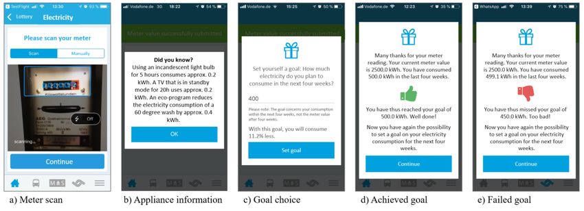
1       Introduction
Policymakers increasingly rely on tools that leverage insights from psychology and behavioral eco-
nomics to affect people’s behavior. These mostly non-pecuniary incentives, referred to as “nudges,”
simplify choice environments and help individuals to implement privately or socially desirable ac-
tions. While nudges have been shown to affect behavior in a large variety of studies, the question
of how these interventions perform at scale often remains unanswered. Understanding the scala-
bility of nudges is arguably of fundamental importance for cost-benefit analyses of nudges and the
optimal choice of policy instruments.
     This study investigates how an underexplored energy conservation nudge performs when im-
plemented as a large-scale policy intervention. The design of the nudge is motivated by a young
literature showing that prompting people to set themselves goals and to make plans helps them fol-
low through with desired behavior. Our study is the first to test the role of goal-setting prompts for
energy conservation in a randomized controlled trial. To take the intervention to scale, we coop-
erate with a large public utility and a specialized IT company and develop an energy savings app
accessible to the majority of the German population.
     Within this app, we randomize a goal-setting feature that prompts users to set themselves en-
ergy consumption targets for the upcoming month. In addition, we randomize a financial incentive
that allows us to monetize the effect of the goal-setting prompt on consumer welfare. We then
promote the rollout of the developed technology through a mass-marketing campaign and a set of
sizable financial incentives. To maximize the chances of successful technology diffusion, we rely
on established industry experts in creating and promoting the mobile app.
     We observe behavior over a total period of seven months, with the following main results. First,
app utilization is strikingly low despite substantial efforts in promoting the app. Second, we find
a precisely estimated null effect of the goal-setting prompt on electricity consumption across all
observed periods. The nudge does not affect behavior, although users set themselves meaningful
goals that are highly predictive of future consumption. Poor targeting properties of the app might
explain the null effect of the nudge. As a complementary survey shows, marginal consumers are
characterized by an already low baseline energy consumption and high levels of energy-related
knowledge. Further, the average marginal consumer is neither present-focused nor loss averse, two
features commonly used in the theoretical literature to explain how goal setting affects behavior
(Koch and Nafziger 2011, Hsiaw 2013).
     Third, we find that the goal-setting nudge causes disutility to consumers, as it significantly
reduces app utilization. Based on a simple theoretical model and experimentally induced price
variation, we estimate that consumers are willing to give up 7.41 EUR to avoid the nudge. Adding
up changes in consumer surplus and nudge provision costs, the nudge causes a large deadweight
loss of 48 EUR per user over a period of only four weeks. These results cast doubt on the prospects
of mobile technologies as cost-effective scaling devices for behaviorally-motivated energy policies.
     Our study makes three main contributions. It is the first study that uses randomly assigned
goal-setting prompts to evaluate its causal effect on energy conservation. Based on the literature,
prompting people to make plans and set goals has shown to help them reduce smoking (Armitage
and Arden 2008), eat healthier (Achtziger, Gollwitzer, and Sheeran 2008), get vaccinated (Milkman
et al. 2011), and vote during elections (Nickerson and Rogers 2010).1 An overview article of the
effectiveness of plan-making by Rogers et al. (2013) concludes that goal-setting prompts should
    1
    There are also few studies that find no effect of planning prompts. For instance, a recent study by (Carrera et al.
2018) asks gym visitors to make plans and estimates a precise null effect of plan-making on gym visits.

                                                          1
play a larger role in public policy. It is therefore a natural step to analyze the role of these promising
interventions in encouraging resource conservation and combating climate change.
    Previous behavioral interventions have proven to be effective tools to reduce resource consump-
tion, such as the widely used social norm comparisons (e.g., Allcott 2011, Ferraro, Miranda, and
Price 2011, Ferraro and Price 2013, Dolan and Metcalfe 2015, Pellerano et al. 2017, Andor et al.
2018, and many others). In the area of goal-setting prompts, we are aware of only one related
study on self-set energy consumption goals. Harding and Hsiaw (2014) use an event study design
to evaluate the effects of an energy savings program in the United States that asked households to
set themselves a target for their electricity consumption. The study finds that self-set goals reduced
consumption by, on average, 8 percent in the short term, but identification hinges on the assumption
that the timing of program take-up is quasi-random. Our estimated confidence intervals rule out
these optimistic treatment effects. Interestingly, we estimate similar saving effects of our interven-
tion if we use the same event study design for our treatment subjects. This implies that at least for
our sample, an event study design fails to identify the causal effect of goals on consumption.
    Second, we add to the emerging literature on the scalability of policy interventions by answering
the following questions: how do goal-setting nudges perform at scale, and are mobile devices an
appropriate scaling device for behaviorally-motivated interventions? Policymakers often need to
base their decisions on studies from small-scale and highly selected samples, which may yield
disappointing results when the intervention is brought to scale (Al-Ubaydli, List, and Suskind 2017,
Al-Ubaydli, List, and Suskind 2019, Czibor, Jimenez-Gomez, and List 2019, DellaVigna and Linos
2020). Our study directly mimics a large-scale policy intervention, targets a representative sample
of households, and thereby circumvents many of the issues that inflate treatment effect estimates.
    We also provide first evidence how smartphones perform in scaling up energy policies. The
medical literature has identified nudges on smartphones as one of the most promising interventions
to improve people’s behavior at scale. Comprehensive overview articles by Vervloet et al. (2012)
and Sarabi et al. (2016) conclude that smartphone applications that include reminders increase pa-
tient compliance with medication intake in the vast majority of the existing studies. The remarkable
success of digital interventions in medicine has led economists to advocate for more studies that
use smartphones for behavioral policy interventions (Al-Ubaydli et al. 2017). Mobile phones are
particularly attractive for scaling up interventions, as they are easy to use and are accessible to the
majority of the population in most countries. Marginal costs of treating subjects are often close
to zero because once a mobile app is developed, it is nearly costless to use. Our understanding
of how these digital technologies can help people to follow through with plans is very limited de-
spite the fact that there is substantial demand for goal-setting apps. Two examples are apps such
as “Goal Meter” or “Goalmap,” which have over 1.1 million downloads combined in the “Android
Playstore.”
    Third, our experiment joins a small set of studies estimating the welfare effects of nudges and
provides the first estimate of the welfare effects of goal-setting prompts. Understanding how nudges
affect consumer surplus and social welfare is fundamental for the identification of optimal policy.
In our setting, a complete cost-benefit calculation must not only weigh the energy cost savings
to consumers with the nudge provision costs. Such a comparison yields misleading conclusions
because it does not fully take into account how the nudge changes consumer utility. For example,
the nudge may yield direct disutility to consumers by pressuring them to save energy. It may also
cause consumers to give up energy service consumption they would otherwise enjoy. To capture
the full effect on consumer well-being, it is therefore crucial to obtain an estimate of their valuation
of the nudge.

                                                    2
For this purpose, we develop a simple model of technology adoption and goal-setting nudges to
derive sufficient statistics to estimate consumers’ willingness-to-pay for the nudge and the resulting
welfare implications. In the experiment, we randomly offer users of the mobile app a lottery if they
continue to use it. The lottery effectively creates exogenous variation in the opportunity cost of
using the app. Comparing app usage between subjects who receive the lottery treatment and those
who receive the goal-setting prompt allows us to approximate the average willingness-to-pay for
the nudge.
We find that the average consumer is willing to give up a large amount of 7.41 EUR to avoid the
nudge. This estimate compares negatively to the prominent social comparison nudges that show
households their peers’ energy consumption (Allcott 2011). Allcott and Kessler (2019) estimate
an average willingness-to-pay of up to USD 4.36 (around 3.93 EUR) for a bundle of four compar-
ison letters. The stark difference in willingness-to-pay in our study highlights the importance of
estimating structural parameters of behavioral models to advance our understanding of how differ-
ent nudges affect utility. Our study is the first to allow for a quantitative comparison between the
welfare effects of underexplored energy conservation nudges to these well-established social com-
parison interventions that are widely employed by policymakers across the world. Only a handful
of other studies have taken a structural approach to behavioral economics to natural field experi-
ments: DellaVigna, List, and Malmendier (2012), DellaVigna et al. (2016), and Butera et al. (2019)
who estimate social preferences; and Rodemeier and Löschel (2020) who estimate informational
biases.2
We structure the presentation of our study as follows. Section 2 describes the experimental
design, the energy app, and the technology diffusion strategy. Section 3 presents reduced-form
results and underlying mechanisms. In Section 4, we estimate the welfare effects of the goal-setting
nudge based on a simple theoretical model. Section 5 discusses our results in relation to previous
evidence. Section 6 concludes.
2 Experimental Design
The experiment was conducted in cooperation with the utility provider of the municipality Münster,
a German city with over 310,000 inhabitants. The utility is a subsidiary company of the munici-
pality and is the default provider in the area, supplying about 80 percent of the households in the
municipality. The experiment spans over a total period of seven months and was implemented in
2018. In the following, we first lay out the design of the mobile app and our treatment. We then
elaborate on how the technology was diffused. The experimental design was pre-registered at the
AEA RCT Registry.3
2
DellaVigna (2018) provides an overview of studies estimating structural behavioral parameters using lab, field,
and observational data. Resulting policy implications of these models are also discussed in Bernheim and Taubinsky
(2019).
3
The trail number is AEARCTR-0003003. When we pre-registered the experiment, we intended to have one addi-
tional treatment arm, in which subjects could re-adjust their pre-set goal at any point in time. Since the first month of
our experiment was the same for all treatments, we were able to adjust our design based on the surprisingly low sign-up
rate. We decided to drop this additional treatment arm to have enough statistical power to identify the causal effect of
goals on energy conservation.
32.1 The Energy App
Our experiment intends to use a promising behavioral intervention and take it to a large scale.
Mobile devices are often considered suitable scaling devices, as they are easily accessible by the
majority of the population. For this reason, we developed a mobile app that integrated a goal-
setting feature prompting users to set themselves energy consumption targets. To causally identify
the effect of a goal-setting feature on energy consumption, the availability of the feature is randomly
assigned among app users. The randomization of the treatment also implies that the app needs to
include other desirable features such that users in the control group find it worthwhile to use. The
app we developed therefore provided two useful features to every user irrespective of treatment
assignment.
First, the app allowed households to scan their meter with their phone and to submit the meter
reading to the utility electronically. This is a useful feature in the German context because the vast
majority of German households do not have smart electricity meters. For meter readings, they are
required to schedule an annual meeting with a representative of the utility who then reads the elec-
tricity meter manually. The app circumvents the hassle of manual meter readings by allowing for an
electronic submission. As depicted in Figure 1a), the developed feature automatically recognizes
and reads the electricity meter if the user points her phone’s camera toward the meter. The user then
only needs to confirm the scan by clicking a button to upload the data to the utility provider’s server.
In case the user experiences technical issues with the scanning process, she can also manually enter
the meter value. However, the app always takes a picture of the meter so that the self-reported meter
value can be verified. Both the digital scans and the actual pictures are available to us.
Second, the app provides simple information on the electricity usage of various household ap-
pliances. Figure 1b) shows a screenshot of the information translated into English. This information
is provided to all subjects irrespective of the experimental group assignment. Providing consumers
with information becomes especially important for the treatment group because saving goals are
likely to only affect consumption if subjects can set meaningful targets and know how to save en-
ergy in the first place. Of course, the information provided may also affect consumption without the
goal-setting feature such that subjects in the control group alter their behavior. Our study therefore
identifies the causal effect of a goal-setting nudge when consumers are informed about the energy
consumption of their appliances. This also means that our design avoids the rather uninteresting
interpretation that goals may simply not affect behavior because people do not understand how
choices map into outcomes.
Figure 2 gives an overview of the experimental timeline. For each app user, the experiment
lasts for four experimental periods, where each period corresponds to 30 days. Upon signing up for
the app, users get randomly assigned to a control and a treatment group with equal probabilities of
one-half. Users need to enter their meter number, zip code, and meter type to exclude the possibility
that the same household participates with multiple devices.4 Participants then conduct a first digital
meter reading with their phone. After subjects have done the first scan, they are informed that the
next scan is due in 30 days. They are given the option to automatically save the due dates of all
upcoming meter scans in the calendar on their phone. As we will discuss in more detail in the
next section, subjects gathered a lottery ticket for every regular meter scan they submitted. The
lottery assured that meter scans were incentivized for all subjects. Throughout the experiment, all
participants received reminders to scan their meter one day before, one day after, and exactly on the
4
The combination of meter number and zip code uniquely identifies a household. The meter type is either a regular
meter or an HT-NT meter. An HT-NT meter records peak electricity consumption separately from off-peak consump-
tion. This information is needed for the scanner functions, as with an HT-NT meter, two scans have to be made.
4due date. We offered participants a grace period to scan their meter from two days before the due
date to two days after the due date. If participants failed to scan the meter within this grace period,
the scanning function was deactivated until another 26 days had passed. After this deactivation
period, they could continue to use the scanning function.
We call the first experimental period our baseline period since these 30 days are identical for
treatment and control. After having completed the second scan after 30 days, participants in the
treatment and control groups receive the aforementioned information on the energy consumption
of different appliances. Afterwards, participants in the treatment group are asked to set themselves
an energy consumption goal for the upcoming 30 days. Figure 1c) shows the goal-setting screen.
Participants enter their desired consumption in kilowatt-hours for the next 30 days. The app also
tells the subject how the consumption goal translates into percentage savings relative to the baseline
period, allowing them to try out different values and get a feeling for a realistic consumption goal.
After the third scan has been submitted, participants in the treatment group are informed of
whether they have reached their goal. If they consumed less than or equal to the planned amount,
they are congratulated and are shown a “thumbs up,” as depicted in panel d) of Figure 1. If they fall
short of their goal by consuming more than intended, they are shown a ”thumbs down” (see panel
e)). Subjects are always also told how many kilowatt-hours they consumed and how this compares
to their target consumption. Afterwards, participants set a new goal for the next 30 days.
The control group does not have this goal-setting feature and just completes the third scan.
In experimental period 4 we randomize an additional treatment among all subjects that provides
a financial incentive to save energy (see Figure A.5 for a screenshot). This “energy saving subsidy”
treatment appears immediately after the fourth scan has been submitted and after a subject has
potentially set a goal for the final period. Specifically, with a probability of one-half, the user is
informed that she participates in a lottery. If she wins the lottery, she receives 1 EUR per kilowatt-
hour saved in month 4 relative to her electricity consumption in month 3. The total amount a
subject may receive from saving energy is limited to 100 EUR. Prizes are paid out in the form
of vouchers for the online shop Amazon.com. The lottery draws 15 users with equal probability
(and no replacement) from the pool of eligible users, which results in a winning probability of
approximately 1.85 percent. The winning probability is the same for every eligible user and is
communicated to the subject. With an average electricity price of 0.30 EUR per kWh, our savings
subsidy corresponds to an increase in the expected electricity price of approximately 6.1 percent.
Thus, there are a total of four experimental groups in the last period: the control group with and
without the savings subsidy and the goal-setting group with and without the savings subsidy. As
we will show in Section 4, the savings subsidy enables us to estimate users’ willingness-to-pay for
the nudge.
Finally, participants are reminded of the fifth and last scan. After completing this last scan, all
of them are invited to an online survey. The survey elicits individual characteristics, qualitative
statements about goal-setting behavior, and measures of electricity price beliefs, loss aversion, and
present-focus. We use this survey to investigate underlying behavioral mechanisms of the treatment
effects.
5Figure 1: Screenshots of Energy App
Note: The figure shows English translations of screenshots of the Energy App. For the original version in German
see Figure A.1.
Figure 2: Experimental Design and Timeline
62.2 Technology Diffusion
The energy app is easily accessible and intentionally simple to use for anyone capable of operating a
smartphone, and it therefore has the potential to be used by the majority of the population. However,
the diffusion of the technology may be slow if the app is not properly marketed. To maximize the
chances of large-scale diffusion, we worked closely together with industry experts. Specifically, the
design of the app was developed by an established IT company specialized for developing mobile
apps. The app’s promotion was designed by both an external marketing agency and marketing
experts of the utility who have experience with the successful rollout and implementation of energy
technologies.
We view the close cooperation with industry experts as a realistic simulation of how govern-
ments would ideally implement and scale up behavioral interventions: they partner with large play-
ers in the industry and leave much of the app’s design and marketing strategy to industry experts.
For our study, this approach also avoids the concern that the technology simply fails to deliver
because its creation and promotion was entirely designed by researchers not trained for these pur-
poses. Whenever we advertised the app, we were careful to only mention the features that were
available to all users and not the randomized treatments.
The diffusion strategy consists of three main steps. First, the energy app is integrated into
a larger and widely used mobile application. The “münster:app” has been downloaded by over
122,000 smartphone users and involves functions such as real-time information on changes in bus
schedules, notifications of free parking spots downtown, and local news.5 The integration of the
energy app into the larger münster:app makes its usage particularly easy, as many households do
not even have to download a new application. All of the münster:app users were notified about the
new features by a push message on their phone and by a large banner displayed on the app’s landing
page.
Second, a promotion campaign targeted the entire municipality. Over 69,000 utility customers
received direct and personalized mails promoting the app (see Figure A.3), and a popular local
radio station played frequent advertisements. As shown in Figure A.2, 14,000 flyers were attached
to annual electricity bills sent by mail. The same flyers were put into a print ad in a local newspaper,
which was then distributed to 18,000 households. Another local newspaper with 48,000 prints
announced the new app, and the social media outlets of the local utility advertised the app. The
main student canteen with around 1,600 visitors per day displayed advertisement posters and flyers.
An additional 4,000 flyers were handed out by research assistants either at public spaces or by going
from door-to-door.
Third, we financially incentivized the use of the app (see Figure A.4 for a screenshot). Every
app user receives a 45 EUR voucher for an online shop of energy-efficient household lighting if
she completes all five meter scans and the online survey. In addition, all users (irrespective of
how many scans they submit) participate in a lottery with various prizes such as holiday trips worth
1,000 EUR, Apple iPads, and 100 EUR vouchers for local activities. The total amount of the lottery
prizes is 6,000 EUR. As previously mentioned, the chances to win in the lottery can be increased
by conducting the digital meter readings: for every regular scan participants send in, they gather
one additional ticket for the lottery. Subjects who submit all regular scans therefore gather five
additional lottery tickets.6
5
The münster:app is run by the local utility provider and is available both through the Google Play Store and the
Apple App Store.
6
The lottery to encourage participation is independent of our randomly assigned Pigouvian lottery in period 4 that
incentivizes energy savings.
72.3 Sample
Table 1 presents the summary statistics of our sample. A total of 1,627 participants signed up and
sent in the first scan. Using information on the meter type, we know whether subjects have a double
tariff involving different nighttime and daytime electricity prices. Around 3 percent of the sample
have such a contract, and these subjects are balanced between the treatment and control groups.
Meters also vary in how they record electricity consumption and may have different decimal places
and numbers of digits before the decimal point. Both of these variables do not significantly differ
between treatment and control.
The baseline electricity consumption is calculated as the difference between the second and
first meter scan. Since not every subject submits a second meter scan, baseline consumption is
not available for all subjects who signed up. Around 50 percent of those who signed up submitted
two or more scans. Importantly, the probability to submit a second scan does not differ between
treatment and control. In total, we have information on baseline electricity consumption for 844
subjects, who consume around 190 kWh, on average, in the baseline month. Baseline consumption
also does not significantly differ between the treatment and control groups. Importantly, baseline
consumption is far below the German average of 264 kWh for the respective month.7 This suggests
that the energy app is attracting consumers with an already low baseline energy consumption and
might imply poor targeting—a point we turn to later in more detail.
Note also that the number of consumers taking up the app is relatively low given the substantial
efforts we made in recruiting participants. Since every subject might have received a variety of
advertisements, we cannot pin down the true response rate. However, we can create a very conser-
vative upper bound on the response rate. Since at least 83,000 individual households were contacted
through direct mailing or flyers with their energy bill, the most optimistic response rate is 1.96 per-
cent. This rate indicates a very low demand for an app related to energy consumption, especially
given our mass-marketing campaign and that participation was financially incentivized through 45
EUR vouchers and a lottery with sizable prizes.
To assure that our electricity data are reliable, our research assistants verified every meter scan.
In particular, they compared the value reported by the digital scan (or the manual data entry by
the user) with the pictures that the app made of the meter. Of a total of 3,610 meter scans, the
research assistants were not able to verify 297 scans (e.g., because these scans did not match the
pictures). In Table A.1 in the Appendix we present results from a regression of the probability to
report non-verifiable meter scans on treatment and find no significant effect. We therefore drop
these observations from our analysis. We also drop four users who have a missing first scan, which
technically should not be possible and does not allow us to calculate baseline consumption.
7
The annual electricity consumption of an average German household is 3,111 kwh (Federal Statistical Office of
Germany 2019). To adjust for seasonal variation in consumption, we use the weights calculated for national load
profiles for different months of the year in Fünfgeld and Tiedemann (2000). In the month of April, load profiles are
about 8.5 percent of annual consumption, resulting in an average consumption of 264 kwh for the month of April.
8Table 1: Summary Table
Control Treatment Difference
Double tariff (1 = yes) 0.036 0.029 –0.008
(0.187) (0.167) (0.009)
Decimal places of meter 1.046 1.049 0.002
(0.342) (0.398) (0.018)
Number of digits before decimal point 5.806 5.833 0.027
(0.605) (0.615) (0.030)
Submitted at least two scans (1 = yes) 0.527 0.509 –0.017
(0.500) (0.500) (0.025)
Baseline consumption (in kWh) 188.466 193.996 5.530
(109.235) (123.006) (8.384)
N 824 434 803 410 1,627 844
Note: This table presents the mean of observable variables for the treatment and control group and the difference in
means between these groups. Standard deviations for control and treatment are reported in parentheses. For the
last two columns, standard errors of the differences are reported. Information on meter characteristics is available
for everyone who signed up for the energy app. Information on baseline electricity consumption is available for
anyone who scanned their meter at the beginning and end of period 1.
3 Reduced-Form Results
3.1 Effect on Extensive Margin: Technology Adoption
We begin by analyzing subjects’ utilization choice of the technology. In every experimental period
e ∈ {1, 2, 3, 4}, the subject has the choice to actively use the app and submit a scan or to not
use the app. We call the utilization choice the extensive margin. We code the outcome variable
U tilizationie such that it equals one if subject i submitted a meter scan at the beginning and at the
end of period e. If the subject did not submit the scan at the beginning or at the end of the period,
the outcome equals zero. To investigate how the treatments affect utilization choice, we estimate
the following linear probability model:
U tilizationie = αe + βe Gie + 1e=4 (γSi + δ × Si × Gie ) + ie , (1)
where Gie equals one if subject i was in the treatment group in period e and zero otherwise. The
average baseline probability to use the app in period e is given by αe , and the error term is denoted
by ie . In period 4 we also randomized the savings subsidy, for which we assign the treatment
dummy Si . The coefficient γ is the treatment effect of the savings subsidy on utilization, and δ
measures the interaction effect of the subsidy with the nudge.
Table 2 reports the results. Around 52 percent of subjects in the control group who signed up
also submitted the second scan and therefore count as being part of period 1. For period 1, the dif-
ference in utilization between treatment and control is small and statistically insignificant, which is
unsurprising given that period 1 was identical for subjects in both groups. The probability to use the
app in the following periods becomes dramatically smaller for both treatment and control subjects.
In the control group, only 29 and 23 percent use the app in periods 2 and 3, respectively. For these
periods, the treatment coefficient of the goal-setting nudge is negative but remains economically
9small and statistically insignificant. This provides evidence of no selection on the extensive margin
during the first two treatment periods and suggests we can causally identify the effect of the nudge
on electricity consumption among users.
Columns 4 and 5 report the effects of the nudge and the subsidy on utilization in period 4. While
column 4 shows pooled effects, column 5 interacts the subsidy with the goal-setting nudge. In the
pooled model, the goal-setting nudge decreased the utilization probability by 4.2 percentage points.
The effect is statistically significant at the 5 percent level. By contrast, the savings subsidy involves
an increase in the utilization probability of 2.9 percentage points. While the effect is not statistically
significant at conventional levels, the t-statistic of 1.45 is relatively large. An independent t-test
shows that the treatment effect of the nudge and the subsidy are significantly different at the 1
percent level. Column 5 reports an even larger negative treatment effect of the nudge and a slightly
smaller effect of the subsidy in isolation. When the nudge is combined with the subsidy, subjects
are 1.6 percentage points more likely to use the app than when they are only treated with the nudge.
Overall, results from period 4 suggest that the goal-setting prompt sufficiently pressured or
disturbed some of the subjects such that they stopped using the app.8 Compensating consumers
with the savings subsidy reduced this tendency.
Table 2: Effect on Extensive Margin: Probability of Using the App Over Time
(1) (2) (3) (4) (5)
Period 1 Period 2 Period 3 Period 4 Period 4
Goal treatment –0.006 –0.013 –0.014 –0.042∗∗ –0.050∗
(0.026) (0.023) (0.022) (0.020) (0.028)
Savings subsidy 0.029 0.021
(0.020) (0.029)
Goal × subsidy 0.016
(0.040)
Constant 0.517∗∗∗ 0.293∗∗∗ 0.237∗∗∗ 0.190∗∗∗ 0.194∗∗∗
(0.018) (0.017) (0.016) (0.018) (0.020)
N 1,493 1,493 1,493 1,493 1,493
Note: The outcome variable is a dummy for whether a subject submitted the meter scan at the beginning and the end
of the respective period. * p < 0.1, ** p < 0.05, *** p < 0.01. Robust standard errors are in parentheses.
3.2 Effect on Intensive Margin: Electricity Consumption
Before we turn to the treatment effect of the goal-setting nudge on energy consumption, we briefly
describe how subjects set their consumption targets. Specifically, we investigate whether subjects
chose meaningful goals, as this indicates whether subjects engaged with the app and the goal-setting
8
We do not find a significant correlation between failing to achieve the goal and dropping out of the app. While this
correlation does not generally have a causal interpretation, it provides suggestive evidence consistent with the idea that
subjects receive negative utility from the goal-setting prompt directly rather than from a failure to reach the goal.
10Figure 3: Actual Versus Planned Consumption
Note: The graph plots the consumption goals against the actual consumption for the treatment group. The orange line
represents the 45-degree line. To account for outliers, we restrict the graph to the 95th percentile of consumption
goals. Observations from all three treatment periods are included.
prompt. If consumption goals are meaningful, we would expect them to be correlated with actual
consumption. By contrast, if subjects just set goals irrespective of their true consumption, the
correlation would be zero. Figure 3 plots the consumption goal (planned consumption) for a month
against the actual consumption of that same month. We also plot the 45-degree line indicating when
planned and actual consumption are equal. To adjust for outliers, we exclude the top 5 percent of
goals.
Visual inspection reveals a striking correlation between planned and actual consumption. Many
subjects choose goals that are highly predictive of their consumption. The figure also shows that
there is a non-negligible share of consumers who chooses consumption goals equal to zero. In
principle, a zero consumption goal is feasible to reach (e.g., when subjects go on vacation) but is
more than unlikely to be a realistic goal for this many households. A more likely interpretation is
that these subjects did not engage with the goal-setting nudge and a value of zero is just a convenient
mental default.
In a nutshell, there are two main groups of subjects in the treatment group. The first one, which
includes the vast majority of the sample, sets meaningful consumption goals that are highly pre-
dictive of their actual future consumption. The second smaller, but non-negligible group, chooses
meaningless goals of zero. Overall, there seems to be a slight tendency for consumers to fall short
of their goal, as most observations lie above the 45-degree line.
The electricity consumption data are a panel data set with four experimental periods. When
11subjects stop using the app and do not scan their meters, electricity consumption is missing. We
therefore have an unbalanced panel, which does not seem problematic for identification in the first
three experimental periods because attrition rates do not systematically differ between treatment
and control. Asymmetric attrition becomes a concern in period 4, in which treatment decreased
the likelihood to use the app (see Section 3.1). Hence, we will use an unbalanced panel but run the
analysis separately with and without the inclusion of period 4. Standard errors will be clustered at
the subject level. Our empirical model is
log(kW hiet ) = Ai + Ee + Tt + τe Gie + γt Sie + iet ,
where log(kW hiet ) is the natural logarithm of participant i’s electricity consumption in experimen-
tal period e and calendar month t. We follow the literature in energy economics and logarithmize
electricity consumption, but this does not change the qualitative interpretation of our results. Re-
call that subjects could submit their meter scan up to 2 days before and 2 days after the due date.
We therefore normalize the outcome variable to resemble 30-days consumption.9 The variables
Gie ∈ {0, 1} and Sie ∈ {0, 1} indicate the nudge treatment and savings subsidy in experimental
period e, respectively. Individual fixed effects and experimental period fixed effects are denoted
by Ai and Ee , respectively. To control for seasonal variation, we also include months fixed effects,
Tt . The consumption recorded in an experimental period e may belong to two calendar months be-
cause subjects do not necessarily start with the experiment on the first day of a calendar month. Tt
therefore comprises a fixed effect for the calendar month in which consumption started and another
fixed effect for the calendar month in which it ended.
The coefficient τe can be interpreted as the approximately average percentage change in electric-
ity consumption in period e caused by the goal-setting prompt at the beginning of the same period.
Table 3 reports the treatment effect coefficients for each period.
9
Specifically, we divide the outcome variable by the number of days that lie between the first and second scan and
then multiply the result by 30.
12Table 3: Effect on Intensive Margin: Electricity Consumption
(1) (2) (3)
Log(kWh) Log(kWh) Log(kWh)
First goal 0.015 0.008
(0.026) (0.024)
Second goal 0.047 0.053
(0.036) (0.037)
Third goal –0.034
(0.046)
Savings subsidy 0.028
(0.040)
Goals (pooled) 0.027
(0.025)
Period 4 consumption included Yes No No
N 1,813 1,538 1,538
Note: The outcome variable is the natural logarithm of electricity consumption measured in kWh. Month and user
fixed effects are included in all regressions. * p < 0.1, ** p < 0.05, *** p < 0.01. Standard errors clustered on
subject level are in parentheses.
The model used to produce results in column 1 includes observations from period 4 and must
be interpreted with caution. We do, however, see that the exclusion of period 4 in column 2 does
not substantially alter results. In both columns, we observe economically small treatment effects of
the first goal-setting prompt of 1.5 and 0.8 percent on electricity consumption, respectively. Both
coefficients are statistically indistinguishable from zero and involve tight confidence intervals. We
can exclude treatment effects smaller than –3.6 percent and –3.9 percent with 95 percent confidence
in columns 1 and 2, respectively. Results are similar for the second goal-setting prompt, but the
lower bounds of the confidence intervals are even closer to zero. Columns 1 and 2 rule out treatment
effects smaller than –2.4 percent and –2.0 with 95 percent confidence.
The third goal prompt involves an insignificant but negative coefficient. The confidence interval
is still small but is larger than for the previous goals, which may be attributable to the fact that we
have few observations for this period. Of course, it may also be a result of systematic selection on
the extensive margin during this period. For the same reason, the coefficient of the savings subsidy
may be imprecisely estimated and/or have no causal interpretation. The coefficient is small and
statistically insignificant.
In column 3 we pool the goal-setting treatments to increase statistical power even further. We
again observe a precisely estimated null effect and can rule out treatment effects smaller than –2.2
percent with 95 percent confidence. Taken all findings together, our results provide considerable
evidence that the goal-setting prompt had no effect on electricity consumption but instead caused
direct disutility to consumers.
133.3 Mechanisms
To investigate underlying mechanisms of the treatment effects, we first need to understand the theo-
retical argument of why goal setting would affect behavior. Economic models on goal setting typi-
cally argue that people set themselves goals to reduce overconsumption resulting from self-control
problems (Koch and Nafziger 2011, Hsiaw 2013). Overconsumption is modeled as an implica-
tion of the well-established β-δ-model (Laibson 1997), in which consumers focus too much on the
present when making choices. Goal setting may then be used as a commitment device for present-
focused agents to mitigate overconsumption. The mechanism is that goals create reference points
to which agents compare their behavior. A crucial component of these models is loss aversion,
meaning that consumers dislike falling short of a self-set goal by a certain distance more than they
value achieving a goal by the same distance.
Our empirical setting features several intertemporal trade-offs that would result in overcon-
sumption for present-focused consumers. Recall that in the German context, energy costs are only
invoiced once a year. While there are exceptions to this billing cycle, 96 percent of our post-
experimental survey respondents state that they receive energy bills annually. Even though every
household pays a fixed monthly payment that should approximately cover monthly energy costs,
this payment is completely independent of current consumption. This means that the costs of in-
creasing current energy consumption is entirely delayed to the (far) future for the majority of our
sample. In addition, externalities create another intertemporal trade-off, as discussed by Harding
and Hsiaw (2014): the negative environmental consequences of excessive resource consumption
only accrue in the future. Even if consumers have altruistic preferences, they may focus too little
on the externalities from energy consumption.
Motivated by these theoretical arguments, we elicited several core model parameters in the post-
experimental survey (see Appendix D). To measure present focus, we use the standard approach of
two incentivized multiple price lists (see, e.g., Coller and Williams 1999 and Cohen et al. 2019).
The first list asks participants to choose between receiving 100 EUR within the next 24 hours or an
alternative amount in one month. The second list includes a trade-off of either receiving 100 EUR
in one month or an alternative amount in two months. In both lists the alternative amount increases
from 100 to 160 EUR across 14 decisions. Importantly, choices are incentivized since one choice
from the two price lists is randomly picked as the actual payment. To ease research expense, we
randomly chose a subset of subjects to be eligible for this actual payment. Randomizing eligibility
has been shown to have no considerable effect on choices, as revealing true preferences remains
optimal (Charness, Gneezy, and Halladay 2016).10
We infer discount rates, denoted δ, by assuming that utility, u(z, ·), is linear in experimental
payments, z, and indifference between the earlier and later payment at the midpoint, z̄, between
the payments at which the participant switches from preferring the earlier amount over the later
amount.11 Under these assumptions, we can calculate discount rates by δ = uut+1 t (z,·)
(z̄,·)
for each
participant and for both price lists. Here, t refers to the earlier date and t + 1 to the later date
10
We communicated to participants a probability of payment, which was selected based on the number of app users
such that in expectation, three participants will be paid. Participants were paid with vouchers for Amazon.com.
11
If the participant switches multiple times between the earlier and later payments, we use the first switching point
to determine the indifference amount. For participants always choosing the later payment, i.e., preferring 100 EUR
later over 100 EUR earlier, we assume indifference at 99.5 EUR. Further, we assume participants always choosing
the earlier payment to be indifferent at 165 EUR. However, whether imposing switching points or excluding never-
switching participants, the average present focus estimate differs only slightly (1.030 when imposing versus 1.006
when excluding).
14of the respective list. The present focus parameter, denoted β, is then identified by the ratio of the
discount rates inferred from the first and second multiple price list (Cohen et al. 2019). β = 1
implies time-consistent discounting, as both discount rates are equal, while β < 1 implies present
focus.
Similarly, we measure loss aversion in our survey from multiple choices between either partici-
pating in a lottery, in which participants can win or lose 150 EUR with equal chances, or receiving a
safe payment. The safe payment varied in 31 decisions from –150 to 150 EUR (Koch and Nafziger
2019). Different to the time preference elicitation, choices are hypothetical. As in Falk et al. (2016),
we use the staircase method to reduce survey length. The staircase method condenses the 31 de-
cisions of the multiple price list into five consecutive choices. This means that the first decision
between lottery and safe payment determines the second choice, the second decision determines
the third choice, etc. Although choices are hypothetical, Falk et al. (2018) show that preferences
elicited from the staircase method correlate with a number of economic outcomes, such as educa-
tion, savings and consumption patterns.
To elicit loss aversion, we follow the standard assumption that u(z, ·) = z if z ≥ 0 and u(z, ·) =
λz if z < 0. Here, λ denotes the degree of loss aversion. If λ = 1, people value gains by the same
amount they dislike losses of equal absolute size, while λ > 1 implies loss aversion. We assume
the amount at which the participant is indifferent between lottery and safe payment, z̄, to be the
midpoint of the two safe payments at which the participant switches from preferring the lottery to
preferring the safe payment.12 With this assumption, we can solve the indifference equation between
z̄−0.5·150
lottery and safe payment, i.e. E[u(z, ·)] = u(z̄, ·), for λ. Specifically, if z̄ ≥ 0, λ = 0.5·(−150) , and
0.5·150
if z̄ < 0, λ = z̄−0.5·(−150) .
Table 4: Behavioral Parameters: Present Focus, Loss Aversion, and Price Beliefs
Representative Average
Sample Average Percentile N Comparison Study
for Comparison
(Std. error) 10th 25th 50th 75th 90th (Std. error)
β 1.030 0.972 1 1 1.013 1.090 353 0.95 Imai, Rutter,
(0.007) (0.02) and Camerer (2019)
(Meta-analysis)
λ 0.826 –0.933 0 0.933 1.25 1.875 352 1.31 Walasek, Mullet,
(0.100) (0.11) and Stewart (2018)
(Meta-analysis)
pmax − pmin 6.658 0 2 4 9 15 193 12.10 Werthschulte
(1.589) (0.519) and Löschel (2019)
(German average)
Note: β denotes the present focus parameter, and λ is the loss-aversion coefficient. pmax − pmin gives the differences
between the maximum and minimum energy price participants believe to pay, measured in cents. Standard errors
of the mean are in parentheses.
Table 4 shows distributional properties of present focus and loss aversion in our sample. The av-
erage subject features a present focus parameter of 1.03 and a loss-aversion parameter of 0.83. Both
12
If participants always preferred the lottery, we assume a switch to the safe payment when offered 160 EUR. Like-
wise, if they always preferred the safe payment, we assume a switch to the lottery when confronted with a safe loss
of 160 EUR. Yet, when we instead exclude never-switching participants, the mean loss-aversion coefficient remains
largely unchanged (0.826 when imposing switching points versus 0.868 when excluding participants).
15estimates are indistinguishable from the rational benchmark of 1. In the absence of measurement
error, these values imply that the average participant is neither present-focused nor loss-averse. We
can see that this is not only true for the average consumer but also for the majority of the survey
sample, as most reported percentiles involve values close to 1. These values markedly differ from
other studies. A meta-analysis by Imai, Rutter, and Camerer (2019) examines 220 estimates from
the literature and estimates an average present focus parameter of 0.95 that is significantly different
from one. For loss aversion, a meta-analysis by Walasek, Mullett, and Stewart (2018) estimates a
median λ of 1.31 and excludes our finding of equal gain-loss weighting with 95 percent confidence.
Other literature reviews regularly report higher loss-aversion parameters (e.g., the average λ of the
studies summarized by Booij, Van Praag, and Van De Kuilen (2010) amounts to 2.069).
Our particular parameter estimates are supported by results from two survey questions, as de-
picted in Figures 4 and 5. As a measure of self-control, subjects were first asked how often they
intend to save energy and then how often they fail to implement these intentions. Possible answers
were “Never,” “Sometimes,” “Often,” and “Always.” We can see in Figure 4 that the distribution
of answers to the first question is oppositely skewed to the distribution of answers to the second
question. While the modal subject intends to save energy on a regular basis, she rarely fails to
implement this intention. These results are also in line with the previously discussed finding that
planned and actual consumption often coincide in the experiment (recall Figure 3).
We also find additional support for the estimated loss-aversion parameter. Specifically, we asked
subjects how they feel when they either receive a refund of 100 EUR by the utility at the end of
the year or when they have to pay an additional 100 EUR to the utility. Answers were ordered on
a 7-point Likert scale from –3 (very bad) to +3 (very good). Figure 5 illustrates the distribution
of responses, and we can see that self-reported emotions are almost perfectly symmetric about
zero. Subjects do not systematically report stronger feelings of losing versus gaining 100 EUR. If
anything, they value gains more than they dislike equal losses.
A theoretically driven explanation for the empirical null effect is therefore that the subject pool is
not characterized by the behavioral biases that typically explain why goal setting affects behavior.
This does, however, not mean that the general population does not feature these biases. Instead,
subject features are likely to be a result of unfavorable self-selection into the pool of app users.13
In fact, this form of systematic self-selection is evident by a number of additional results. For
example, and as previously reported, the baseline consumption of app users is below the national
average, which is important since previous research consistently finds larger energy savings effects
for households with a larger baseline consumption (e.g., Allcott (2011), Andor et al. (2018) ).
In addition, app users appear to have higher levels of “energy literacy” than the average German
household. This becomes evident by another survey question eliciting subjects’ confidence about
the energy price they pay. Subjects were asked to state the minimum and maximum price they think
they pay for electricity. The last row in Table 4 reports the difference between the maximum and
minimum as a measure of confidence. The average participant reports a relatively small interval of
0.07 EUR. To put this into perspective, we compare this estimate to the belief interval elicited in a
nationally representative survey conducted by Werthschulte and Löschel (2019). In their sample the
average deviation between maximum and minimum perceived electricity price is 0.12 EUR (i.e.,
almost twice as large as for our subject pool), suggesting consumers with an already high knowledge
for energy-related topics use the app.
13
Note that a typical issue with small-scale studies is favorable self-selection of subjects into the pool of
participants—a phenomenon Al-Ubaydli et al. (2017) label “adverse heterogeneity”. Favorable self-selection implies
that subjects select on gains such that study participants have larger treatment effects than the overall population.
16Additional evidence for systematic sample selection can be found in the sociodemographics, as
documented in Table A.3 in the Appendix. App users are predominantly male (23 percent female
versus 51 percent nationwide) and are better educated than the average German (76 percent with
a high school degree versus 33 percent nationwide). The average participant is also slightly older
(46 years versus 44 years) and earns a higher income (2,515 EUR per month versus 1,770 EUR per
month). Participating households are even characterized by larger dwellings (107 square meters
versus 98 square meters) and a larger household size than the national average (2.54 persons per
household versus 1.98 persons per household). This means that energy consumption per capita is
far below the average, since the total energy consumption per household was already relatively low.
A plausible explanation is that sample participants consume energy more efficiently than a national
representative household does, consistent with their high level of energy literacy.
Figure 4: Intentions and Self-Control
17Figure 5: Gain and Loss Feelings
In sum, the metrics point at very poor targeting properties of the app. Based on a theoretical
argument, the ideal consumer to target would be loss averse and would have self-control problems
and high levels of baseline energy consumption. Instead we find the opposite: subjects who decide
to use the app are well-informed consumers with rational behavioral parameters and low levels
of baseline energy consumption. More generally, our results highlight the importance of carefully
documenting selection into the pool of study participants in order to understand treatment effects—
an approach advocated by List (2020).
4 Welfare Analysis
4.1 A Simple Model of Technology Adoption
We develop a simple theoretical model that allows us to quantify the efficiency effects of the nudge.
In our experiment, subjects can adjust their behavior on two margins. On the extensive margin,
they choose app utilization j ∈ {a, o}, where a denotes the energy savings app and o the outside
option. On the intensive margin, they potentially choose an energy savings goal (if the feature is
available) and then choose their actual energy consumption. We will solve the model backwards
by first deriving the optimal intensive margin choices conditional on utilization choice and then
deriving the optimal utilization choice on the extensive margin. Since an empirical welfare analysis
requires exogenous price variation, we restrict our theoretical model to the last experimental period,
in which we also varied the expected energy price. We therefore use a static model that applies to
the fourth experimental period.
18You can also read