Weakening of Antarctic stratospheric planetary wave activities in early austral spring since the early 2000s: a response to sea surface ...
←
→
Page content transcription
If your browser does not render page correctly, please read the page content below
Research article
Atmos. Chem. Phys., 22, 1575–1600, 2022
https://doi.org/10.5194/acp-22-1575-2022
© Author(s) 2022. This work is distributed under
the Creative Commons Attribution 4.0 License.

          Weakening of Antarctic stratospheric planetary wave
          activities in early austral spring since the early 2000s:
              a response to sea surface temperature trends
                       Yihang Hu1 , Wenshou Tian1 , Jiankai Zhang1,2 , Tao Wang1 , and Mian Xu1
                        1 KeyLaboratory for Semi-Arid Climate Change of the Ministry of Education,
                            College of Atmospheric Sciences, Lanzhou University, Lanzhou, China
                 2 Southern Marine Science and Engineering Guangdong Laboratory (Zhuhai), Zhuhai, China

                                   Correspondence: Wenshou Tian (wstian@lzu.edu.cn)

                                     Received: 11 May 2021 – Discussion started: 1 June 2021
                      Revised: 21 November 2021 – Accepted: 12 December 2021 – Published: 1 February 2022

       Abstract. Using multiple reanalysis datasets and modeling simulations, the trends of Antarctic stratospheric
       planetary wave activities in early austral spring since the early 2000s are investigated in this study. We find
       that the stratospheric planetary wave activities in September have weakened significantly since the year 2000,
       which is mainly related to the weakening of the tropospheric wave sources in the extratropical Southern Hemi-
       sphere. As the Antarctic ozone also shows clear shift around the year 2000, the impact of ozone recovery on
       Antarctic planetary wave activity is also examined through numerical simulations. Significant ozone recovery
       in the lower stratosphere changes the atmospheric state for wave propagation to some extent, inducing a slight
       decrease in the vertical wave flux in upper troposphere and lower stratosphere (UTLS). However, the changes
       in the wave propagation environment in the middle and upper stratosphere over the subpolar region are not sig-
       nificant. The ozone recovery has a minor contribution to the significant weakening of stratospheric planetary
       wave activity in September. Further analysis indicates that the trend of September sea surface temperature (SST)
       over 20◦ N–70◦ S is well linked to the weakening of stratospheric planetary wave activities. The model simula-
       tions reveal that the SST trend in the extratropical Southern Hemisphere (20–70◦ S) and the tropics (20–20◦ S)
       induce a weakening of the wave 1 component of tropospheric geopotential height in the extratropical Southern
       Hemisphere, which subsequently leads to a decrease in stratospheric wave flux. In addition, both reanalysis data
       and numerical simulations indicate that the Brewer–Dobson circulation (BDC) related to wave activities in the
       stratosphere has also been weakening in early austral spring since the year 2000 due to the trend of September
       SST in the tropics and extratropical Southern Hemisphere.

1   Introduction                                                  R. Zhang et al., 2019) through downward control processes
                                                                  (Haynes et al., 1991), which are useful for extended forecasts
Stratospheric planetary wave activities have important influ-     by using the preceding signals in the stratosphere (e.g., Bald-
ences on stratospheric temperature (e.g., Hu and Fu, 2009;        win and Dunkerton, 2001; Wang et al., 2020).
Lin et al., 2009; Li and Tian, 2017; Li et al., 2018), the po-       The planetary perturbations generated by large-scale to-
lar vortex (e.g., Kim et al., 2014; Zhang et al., 2016; Hu et     pography, convection, and the continent–ocean heating con-
al., 2018), and the distribution of chemical substances (e.g.,    trast can propagate from the troposphere to the stratosphere
Gabriel et al., 2011; Ialongo et al., 2012; Kravchenko et al.,    (Charney and Drazin, 1961) and form stratospheric plane-
2012; J. Zhang et al., 2019). Meanwhile, the stratospheric        tary waves. As the land–sea thermal contrast in the Northern
circulation modulated by planetary waves can exert impacts        Hemisphere is larger than that in the Southern Hemisphere
on tropospheric weather and climate (e.g., Haigh et al., 2005;    and produces stronger zonal forcing for the genesis of strato-

Published by Copernicus Publications on behalf of the European Geosciences Union.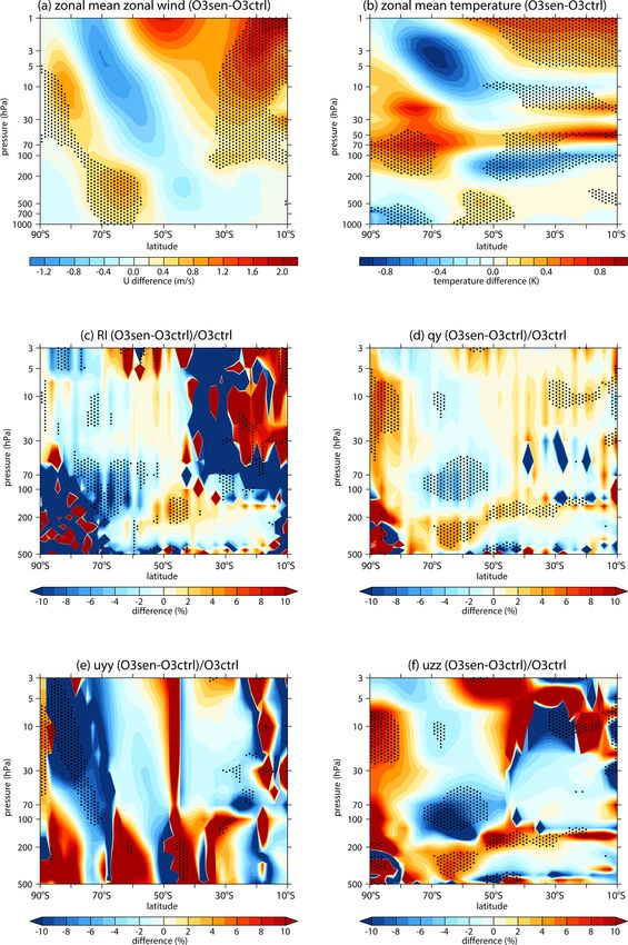
1576                     Y. Hu et al.: Weakening of Antarctic stratospheric planetary wave activities since the early 2000s

spheric waves, the majority of attention has been given to       ison Project (CMIP5) models, Barnes et al. (2014) proposed
wave activities and their impacts on weather and climate in      that, since the early 2000s, the tropospheric jet and dry zone
the Northern Hemisphere (e.g., Kim et al., 2014; Zhang et        edge no longer shift poleward during austral summer due to
al., 2016; Hu et al., 2018). However, planetary wave activi-     the ozone recovery. Banerjee et al. (2020) analyzed the ob-
ties in the Southern Hemisphere also play an important role      servations and reanalysis datasets. They found that, follow-
in heating the stratosphere dynamically (e.g., Hu and Fu,        ing the ozone recovery after the year 2000, the increase in
2009; Lin et al., 2009), which suppresses polar stratospheric    the SAM index and the poleward shifting of tropospheric jet
cloud (PSC) formation and ozone depletion (e.g., Shen et al.,    position and the Hadley cell edge all experienced a pause.
2020a; Tian et al., 2017). The Antarctic sudden stratospheric    Their results suggest that ozone depletion and recovery have
warming (SSW) that occurred in 2002 (e.g., Baldwin et al.,       made important contributions to the climate shift that oc-
2003; Nishii and Nakamura, 2004; Newman and Nash, 2005)          curred around the year 2000 in the Southern Hemisphere.
and 2019 (e.g., Yamazaki el al., 2020; Shen et al., 2020a, b)       However, some previous studies have reported zonally
was associated with a significant upward propagation of the      asymmetric warming patterns in Antarctic stratosphere,
wave flux. Such episodes are extraordinarily rare in the his-    which are generated by increased planetary wave activities
tory, and the one in 2019 contributed to the formation of the    during austral spring from the early 1980s to the early 2000s
smallest Antarctic ozone hole on record (WMO, 2019). In          (Hu and Fu, 2009; Lin et al., 2009). Note that the Antarctic
addition, some studies reported that wildfires in Australia at   stratosphere was experiencing radiative cooling in the same
the end of 2019 are related to negative phase of the Southern    period due to ozone depletion (e.g., Randel and Wu, 1999;
Annular Mode (SAM), which was induced by the extended            Solomon, 1999; Thompson et al., 2011). The increase in
influence of the SSW event that occurred in September (Lim       stratospheric planetary wave activities cannot be explained
et al., 2019; Shen et al., 2020b). In a word, the Antarctic      by ozone decline because the acceleration of stratospheric
planetary wave activities are important for the stratosphere–    circumpolar wind caused by radiative cooling induces more
troposphere interactions and climate system in the Southern      wave energy to be reflected back to the troposphere (e.g.,
Hemisphere.                                                      Andrews et al., 1987; Holton, 2004). Hu and Fu (2009) at-
   Long-term observations in the Antarctic stratosphere show     tributed the increase in the Antarctic stratospheric wave ac-
a significant ozone decline from the early 1980s to the early    tivities to the sea surface temperature (SST) trend from the
2000s due to the anthropogenic emission of chlorofluorocar-      1980s to the 2000s. Their results indicate that, in addition
bons (CFCs; WMO, 2011) and a recovery signal since the           to ozone change, other factors such as changes in SST also
2000s because of phasing out CFCs in response to Montreal        contribute to climate change in the Southern Hemisphere.
Protocol (e.g., Angell and Free, 2009; Krzyścin, 2012; Zhang    Moreover, the phase of Interdecadal Pacific Oscillation (IPO)
et al., 2014; Banerjee et al., 2020). The Antarctic strato-      also changed at around the year 2000 (e.g., Trenberth and Fa-
spheric ozone depletion and recovery have important impacts      sullo, 2013). SST variation influences Rossby wave propaga-
on climate in the Southern Hemisphere. The ozone depletion       tion and tropospheric wave sources and, thereby, indirectly
cools the Antarctic stratosphere through reducing the absorp-    affects stratospheric wave activities (e.g., Lin et al., 2012;
tion of radiation and leads to the strengthening of Antarc-      Hu et al., 2018; Tian et al., 2017). The questions here are
tic polar vortex during austral spring (e.g., Randel and Wu,     as follows: (1) has the trend of stratospheric planetary wave
1999; Solomon, 1999; Thompson et al., 2011). The anoma-          activity in the Southern Hemisphere been shifting since the
lous circulation in the Antarctic stratosphere during austral    2000s? (2) What are the factors responsible for the trend
spring exerts impacts on tropospheric circulations (e.g., in-    of Antarctic stratospheric planetary wave activity since the
tensification of SAM index, poleward shift of tropospheric       2000s?
jet position, and expansion of the Hadley cell edge) in the         In this study, we reveal the trend of Antarctic planetary
subsequent months (e.g., Thompson et al., 2011; Swart and        wave activity in early austral spring since the 2000s based
Fyfe, 2012; Son et al., 2018; Banerjee et al., 2020) and in-     on multiple reanalysis datasets. We also conduct sensitivity
fluences the distribution of precipitation and dry zone in the   experiments forced by linear increments of ozone and SST
Southern Hemisphere (e.g., Thompson et al., 2011; Barnes         fields since the 2000s to investigate the response of Antarc-
et al., 2013; Kang et al., 2011). Following the healing of the   tic planetary activity to the above two factors. The remainder
ozone loss in the Antarctic ozone hole since the 2000s (e.g.,    of the paper is organized as follows. Section 2 describes the
Solomon et al., 2016; Susan et al., 2019), great attention has   data, methods, and configurations of model simulations. Sec-
been paid to the possible impacts of ozone recovery on the       tion 3 presents the trends of stratospheric and tropospheric
climate system in the Southern Hemisphere (e.g., Son et al.,     wave activities in the early austral spring. Section 4 exam-
2008; Barnes et al., 2014; Xia et al., 2020; Banerjee et al.,    ines the impact of ozone recovery on Antarctic stratospheric
2020). Son et al. (2008) implemented the Chemistry–Climate       planetary wave activity. Section 5 investigates the connec-
Model Validation (CCMVal) to predict the response of the         tions between the trends of SST and stratospheric wave activ-
Southern Hemisphere westerly jet to stratospheric ozone re-      ities. Section 6 discusses the responses of tropospheric wave
covery. Based on phase 5 of the Coupled Model Intercompar-       sources and stratospheric wave activities to SST changes

Atmos. Chem. Phys., 22, 1575–1600, 2022                                           https://doi.org/10.5194/acp-22-1575-2022
Y. Hu et al.: Weakening of Antarctic stratospheric planetary wave activities since the early 2000s                                                   1577

based on model simulations. Major conclusions and discus-
sion are presented in Sect. 7.
                                                                    F (φ) = ρ0 a cos φ(uz v 0 θ 0 /θz − v 0 u0 )                                         (1)
                                                                        (z)                                    −1
2     Datasets, methods, and experimental                           F         = ρ0 a cos φ{[f − (a cos φ)           (u cos φ)φ ]v 0 θ 0 /θz − w 0 u0 }   (2)
                                                                                                                                     (z)
      configurations                                                                                            ∂
                                                                                                   (a cos φ)−1 ∂φ (F (φ) cos φ) + ∂F∂z
                                                                                   ∇ ·F
                                                                     DF =                   =                                                       , (3)
2.1    Datasets                                                                  ρ0 a cos φ                           ρ0 a cos φ

In this study, daily and monthly mean data extracted from           where u, v represent zonal and meridional components of
the Modern-Era Retrospective analysis for Research and Ap-          horizontal wind, w is vertical velocity, θ is potential temper-
plications, Version 2 (MERRA-2; Bosilovich et al., 2015),           ature, a is the Earth’s radius, f is the Coriolis parameter, z is
dataset are used to calculate trends of Brewer–Dobson circu-        geopotential height, φ is latitude, and ρ0 is the background
lation (BDC), tropospheric wave sources, and the Eliassen–          air density.
Palm (E–P) flux and its divergence in September. To verify             The quasi-geostrophic refractive index (RI) is used to diag-
the trend of stratospheric E–P flux, we also refer to the re-       nose the environment of wave propagation (Chen and Robin-
sults derived from the European Centre for Medium-Range             son, 1992). Its algorithm is written as Eq. (4), as follows:
Weather Forecasts (ECMWF) Interim Reanalysis (ERA-                        q̄ϕ

                                                                                      k
                                                                                           2
                                                                                                     f
                                                                                                          2
Interim; Dee et al., 2011) dataset, the Japanese 55-year Re-        RI =      −               −              ,                   (4)
                                                                           ū      a cos ϕ        2N H
analysis (JRA-55; Kobayashi et al., 2015) dataset, and the
National Centers for Environmental Prediction–Department            where the zonal mean potential vorticity meridional gradient
of Energy (NCEP-DOE) Global Reanalysis 2 (NCEP-2;                   q̄ϕ is as follows:
Kanamitsu et al., 2002) dataset.
                                                                                                          f2

                                                                           2           1 (ū cos ϕ)ϕ             ūz
   The observed total column ozone (TCO) data are extracted         q̄ϕ =       cos ϕ − 2               −     ρ0 2 .         (5)
from the SBUV (Solar Backscatter Ultraviolet) v8.6 satellite                a          a    a cos ϕ ϕ ρ0         N z
dataset, which is a monthly and zonal mean dataset on a 5◦
                                                                    H, q, k, N 2 , and  are the scale height, potential vorticity,
grid. Ozone data derived from the MERRA-2 dataset are also
                                                                    zonal wave number, buoyancy frequency, and Earth’s angular
used to calculate TCO.
                                                                    frequency, respectively.
   SST data are extracted from the National Oceanic and At-
                                                                       The Brewer–Dobson circulation driven by wave breaking
mospheric Administration (NOAA) Extended Reconstructed
                                                                    in the stratosphere is closely related to stratospheric wave ac-
Sea Surface Temperature (ERSST) dataset, which is a global
                                                                    tivities. Its meridional and vertical components (v̄ ∗ , w̄ ∗ ) and
monthly mean sea surface temperature dataset derived from
                                                                    stream function (ψ ∗ (p, φ)) are expressed by Eqs. (4)–(6), as
the International Comprehensive Ocean-Atmosphere Dataset
                                                                    follows (Andrews et al., 1987; Birner and Bönisch, 2011):
(ICOADS). The ERSST is on global 2◦ × 2◦ grid and cov-
ers the period from January 1854 to the present. We use the                     v̄ ∗ ≡ v̄ − ρ0−1 (ρ0 v 0 θ 0 /θz )z                                      (6)
latest version (version 5; i.e., v5) dataset to calculate trends                 ∗                       −1
                                                                           w̄ ≡ w̄ + (a cos φ)                (cos φ · v 0 θ 0 /θ
                                                                                                                     z )φ                                (7)
and correlations and the produce SST forcing field for model
                                                                                  p
simulations. More details about this version of ERSST can                        Z
                                                                                    −2π a · cos φ · v̄ ∗ (p 00 , φ) 00
be found in Huang et al. (2017).                                    ψ ∗ (p, φ) =                                   dp ,                                  (8)
                                                                                                g
   In addition, the unfiltered Interdecadal Pacific Oscillation                        0
(IPO) index derived from the ERSST v5 dataset is also used
                                                                    where p is the air pressure, π is the circular constant, and g
in this study. More detailed information about the index can
                                                                    is the gravitational acceleration.
be found in Henley et al. (2015).
                                                                       In Eqs. (1)–(8), the overbar and prime denote a zonal mean
                                                                    and departure from the zonal mean, respectively. The sub-
2.2    Diagnosis of wave activities and Brewer–Dobson               scripts denote partial derivatives. The Fourier decomposition
       circulation                                                  is used to obtain components of Eqs. (1)–(3) with different
Planetary wave activities are measured by the E–P flux (F ≡         zonal wave numbers. Meanwhile, the Fourier decomposed
(0, F (φ) , F (z) )) and its divergence DF . Their algorithms are   components of geopotential height zonal deviations are also
expressed by Eqs. (1)–(3), as follows (Andrews et al., 1987):       used to determine tropospheric wave sources.

                                                                    2.3        Statistical methods
                                                                    The trend is measured by the slope of linear regression based
                                                                    on the least square estimation. The correlation is used to an-
                                                                    alyze statistical links between different variables. In this pa-
                                                                    per, all the time series have been linearly detrended before

https://doi.org/10.5194/acp-22-1575-2022                                                   Atmos. Chem. Phys., 22, 1575–1600, 2022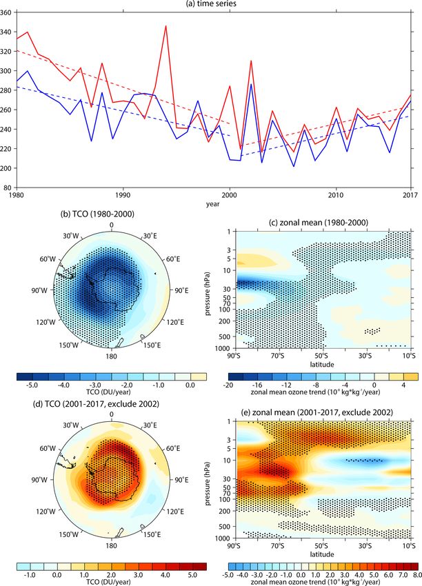
1578                       Y. Hu et al.: Weakening of Antarctic stratospheric planetary wave activities since the early 2000s

calculating correlation coefficients (r) and their correspond-       NHtrop (the extratropical Northern Hemisphere and the trop-
ing significances.                                                   ics; 20◦ S–70◦ N), and the globe (70◦ S–70◦ N). To find sta-
   The change point testing (e.g., Banerjee et al., 2020) is         tistical connections between the trend of SST and that of
used to make sure that the significance of trend or correlation      stratospheric wave activities, we examine the first three lead-
coefficient is not unduly influenced by some particular be-          ing patterns (EOF1, EOF2, and EOF3) and principal compo-
ginning or ending years and, thereby, confirm that the trend         nents (PC1, PC2, and PC3) of SST in the abovementioned six
exists objectively.                                                  regions obtained from empirical orthogonal function (EOF)
   We use two-tailed Student’s t test to calculate the signif-       analysis. In all the six regions, there is always one EOF mode
icances of the trend, correlation coefficient, or mean differ-       that shows great similarity to the spatial pattern of the trend
ence. The result of the significance test is measured by the p       (not shown), as we do not detrend the SST time series when
value or confidence intervals in this paper. p ≤ 0.1, p ≤ 0.05,      the EOF analysis is carried out. Thus, the significance of the
and p ≤ 0.01 suggest the trend, correlation coefficient, or          correlation between the PC time series of that EOF mode and
mean difference is significant at/above the 90 %, 95 %, and          the time series of stratospheric E–P flux can be used as the
99 % confidence levels, respectively. The confidence interval        criterion to determine the statistical connection between the
of trend is shown in Eq. (7), as follows (Shirley et al., 2004):     trend of SST and the trend of stratospheric wave activities.
h                                               i
 b̂ − t1−α/2 (n − 2)σ̂b , b̂ + t1−α/2 (n − 2)σ̂b ,           (9)     2.4   The model and experiment configurations

                                                                     The F_2000_WACCM_SC (FWSC) component in the Com-
where b̂ is estimated value of slope. r
                                      σ̂b is the standard error
                                                                     munity Earth System Model (CESM; version 1.2.0) is
                                           1
                                           2   −1                    used to verify the impacts of SST and ozone recovery on
of slope, and it is written as σ̂b = b̂ · rn−2 , t1−α/2 , (n − 2),
                                                                     tropospheric wave sources and stratospheric wave activi-
which denotes the value of t distribution with the degree of
                                                                     ties in early austral spring. The FWSC component is the
freedom equal to n − 2 and the two-tailed confidence level
                                                                     Whole Atmosphere Community Climate Model, version 4
equal to 1−α (α = 0.90, 0.95 or 0.99). The confidence inter-
                                                                     (WACCM4), with specified chemistry forcing fields (such
val of the mean difference is expressed by Eq. (8) as follows
                                                                     as ozone, greenhouse gases (GHGs), aerosols, and so on),
(Shirley et al., 2004):
                                                                     which have fixed values by default in the year 2000. The
                                       r                             WACCM4 includes active atmosphere, data ocean (run as a
                                      1   1
 X̄ − Ȳ − t1−α/2 (M + N − 2) · Sw ·     + ,                         prescribed component by simply reading SST forcing data
                                       M N                           instead of running ocean model), land, and sea ice. Physics
                                     r
                                       1   1                         schemes in the WACCM4 are based on those in the Com-
 X̄ − Ȳ + t1−α/2 (M + N − 2) · Sw ·     +     ,             (10)
                                       M N                           munity Atmosphere Model, version 4 (CAM4; Neale et al.,
                                                                     2013). The WACCM4 uses a finite-volume dynamic frame-
where, in the following:                                             work and extends from the ground to approximately 145 km
     v                                                               (5.1 × 10⁻⁶ hPa) altitude in the vertical, with 66 vertical lev-
                                                                     els. The simulations presented in this paper are conducted
                  "                                 #
     u              M               N
     u       1      X
                                2
                                   X
                                                  2
Sw = t                 (Xi − X̄) +      (Yj − Ȳ ) . (11)            at a horizontal resolution of 1.9◦ × 2.5◦ . More information
         M + N − 2 i=1             j =1                              about the WACCM can be found in Marsh et al. (2013).
                                                                        Control experiments and sensitivity experiments are con-
Here, X̄ and Ȳ are the sample averages, M and N are the             ducted to investigate the responses of Antarctic stratospheric
numbers of sample sizes with two populations, t1−α/2 (M +            wave activities to SST trends and the ozone recovery trend
N − 2) denotes the value of t distribution, with the degree of       in early austral spring. For the experiments of SST trends,
freedom equal to M + N − 2 and the two-tailed confidence             monthly mean global SST during 1980–2000 derived from
level equal to 1 − α.                                                the ERSST v5 dataset is used as the SST forcing field in
   Previous studies have indicated that SST impact on the            the control experiment (sstctrl). For the four sensitivity ex-
stratosphere shows a spatial dependence (e.g., Xie et al.,           periments (sstNH, sstSH, ssttrop, and sstSHtrop), linear in-
2020). To find out a robust relationship between the trend           crements of SST in different regions in September during
of SST in a specific region and the trend of stratospheric           2000–2017 are used as the forcing field. Ozone, aerosols,
wave activities, we divide the global ocean into three regions,      and greenhouse gases (GHGs) in the control experiment and
namely the SH (the extratropical Southern Hemisphere; 70–            the four sensitivity experiments all have the fixed values
20◦ S), TROP (the tropics; 20◦ S–20◦ N), and NH (the ex-             from the year 2000. For the experiments of ozone recovery
tratropical Northern Hemisphere; 20–70◦ N). Since the im-            trend, monthly mean three-dimensional global ozone during
pacts in different regions might be combined, we also con-           1980–2000, derived from the MERRA-2 dataset, is used as
sider three combined regions named as SHtrop (the extra-             the ozone forcing field in the control experiment (O3ctrl).
tropical Southern Hemisphere and the tropics; 70–20◦ N),             The sensitivity experiment (O3sen) is forced by linear incre-

Atmos. Chem. Phys., 22, 1575–1600, 2022                                               https://doi.org/10.5194/acp-22-1575-2022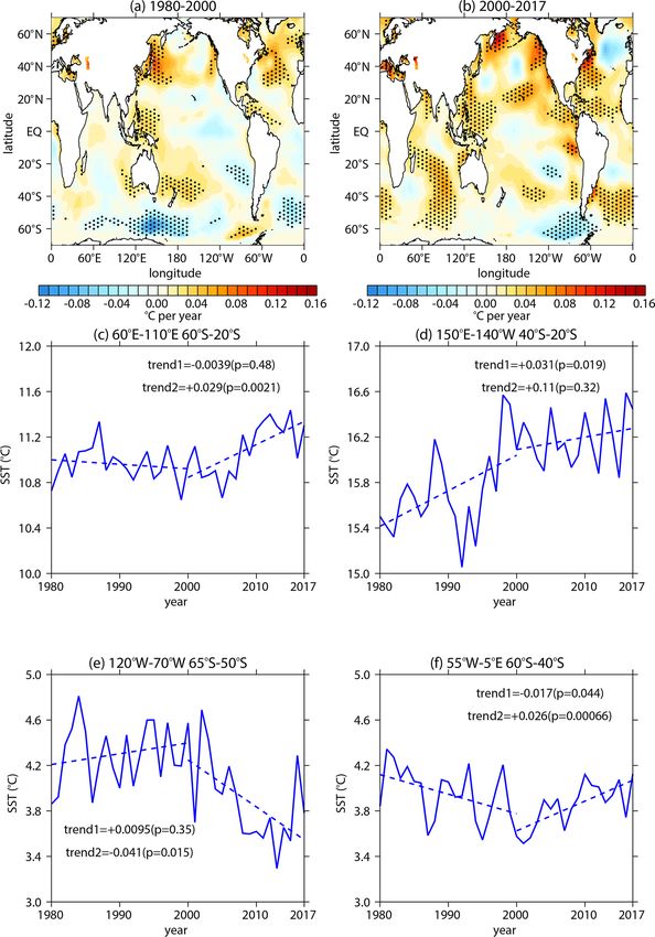
Y. Hu et al.: Weakening of Antarctic stratospheric planetary wave activities since the early 2000s                            1579

ments of ozone in September during 2001–2017. The SSTs in          ous periods, based on four reanalysis datasets (ERA-Interim,
O3ctrl and O3sen both are monthly mean global SST during           MERRA-2, JRA-55, and NCEP-2). Figure 2a (including the
1980–2000. The aerosol and GHG values in the year 2000             year 2002) and b (excluding the year 2002) display the time
are used. These experiment configurations are summarized           series of the area-weighted vertical stratospheric wave flux
and listed in Tables 1 and 2.                                      (Fz) over the Southern Hemisphere subpolar region obtained
   First, we run the FWSC component to randomly gener-             from different reanalysis datasets. Note that the wave flux
ate different initial conditions for 120 years with a free run.    time series obtained from the four reanalysis datasets all
Then, each experiment includes 100 ensemble members that           present a positive trend from the early 1980s to the early
run from July to September and forced by these initial con-        2000s and a negative trend from the early 2000s to present,
ditions from the 21st year to the 120th year in July. The forc-    regardless of whether the extreme value in 2002 is removed
ing fields of SST and ozone are only superposed from July to       or not. The correlation coefficients of the time series between
September. July and August are taken as the spin-up time,          these reanalysis datasets are above 0.9 and statistically signif-
and simulations during this period are discarded. The en-          icant (Table 3), suggesting that the time series derived from
semble mean in September derived from these 100 ensemble           different datasets are consistent with each other. Figure 2c–f
members is regarded as the final result of each experiment. A      show the trends and corresponding confidence intervals cal-
similar approach is implemented for sensitivity experiments,       culated with the four different beginning years (1980, 1981,
in which the forcing fields superposed only in certain months.     1982, and 1983), the four different ending years (2015, 2016,
The same approach has been used in previous studies (e.g.,         2017, and 2018), and the change point years from 1998 to
Zhang et al., 2018).                                               2013. The trends and confidence intervals in Fig. 2g–j are the
                                                                   same as those in Fig. 2c–f, except that the extreme value in
                                                                   2002 is removed. The positive trend from the early 1980s to
3   Trend of planetary wave activities in early austral            the 21st century remains significant, regardless of different
    spring                                                         beginning years and ending change point years (Fig. 2c–j).
                                                                   However, Fig. 2c–f and g–j indicate that the positive value
Figure 1 shows the trends of stratospheric planetary wave          of the trend is decreasing gradually when the period is pro-
activities in the Southern Hemisphere in September during          longed, which is apparently attributed to the negative trend
1980–2000 and 2000–2017, respectively. Note that the ver-          with the beginning change point year of around the year
tical E–P flux entering into the stratosphere over 50–70◦ S        2000. Although the negative trend from the change point year
in September has been increasing during 1980–2000 and is           to the ending year becomes less significant when the value
accompanied by an intensified wave flux convergence in the         in 2002 is removed, it remains significant in some periods,
upper stratosphere (Fig. 1a) that is mainly contributed by the     which is also illustrated in the diagrams of latitude pressure
wave 1 component (Fig. 1b). This feature implies that the          profiles (Fig. S2). Therefore, the weakening of stratospheric
stratospheric planetary wave activities have strengthened in       wave activities in early austral spring since the early 2000s
early austral spring during 1980–2000. A similar result has        has been robust. In this paper, we take the year 2000 as the
been reported in previous studies (Hu and Fu, 2009; Lin et         beginning year of the weakening trend to simplify descrip-
al., 2009). During 2000–2017, however, a vertical propaga-         tions in the following discussion.
tion of stratospheric E–P flux weakened over the subpolar             Figure 3 shows the trends in tropospheric wave sources in
region of the Southern Hemisphere, which was accompanied           September since the year 2000. There is a significant positive
by intensified wave flux divergence in the upper stratosphere      trend of the wave 1 component at 500 hPa geopotential height
(Fig. 1d) that was mainly contributed by the wave 1 compo-         over the southern Indian ocean and a significant negative
nent (Fig. 1e), while the wave 2 component also made certain       trend over the southern Pacific, which form an out-of-phase
contributions (Fig. 1f). Similar features also appear in Au-       superposition on its climatology (Fig. 3b). The trend pattern
gust but are not as significant as those in September (Fig. S1     of the wave 2 component is also out of phase with its cli-
in the Supplement). For this reason, hereafter we focus on         matology, although it is not significant (Fig. 3c). The above
the features in September.                                         features are still maintained when the values in 2002 are re-
   The SSW that occurred in 2002 was accompanied by large          moved (Fig. S3b, c), implying that the southern hemispheric
upward wave fluxes in the stratosphere, which is extremely         tropospheric wave sources in early austral spring have weak-
rare in history and has been studied extensively in previous       ened since the year 2000, which is also reflected in the de-
studies (e.g., Baldwin et al., 2003; Nishii and Nakamura,          crease in the tropospheric vertical wave flux (Figs. 3d, e; S3d,
2004; Newman and Nash, 2005). Since the period with a neg-         e).
ative trend of the stratospheric vertical wave flux is short, it
is necessary to further investigate whether such a negative
trend is artificially influenced by the single year of 2002.
Therefore, following Banerjee et al. (2020), we use a change
point method to test the significance of the trend during vari-

https://doi.org/10.5194/acp-22-1575-2022                                           Atmos. Chem. Phys., 22, 1575–1600, 2022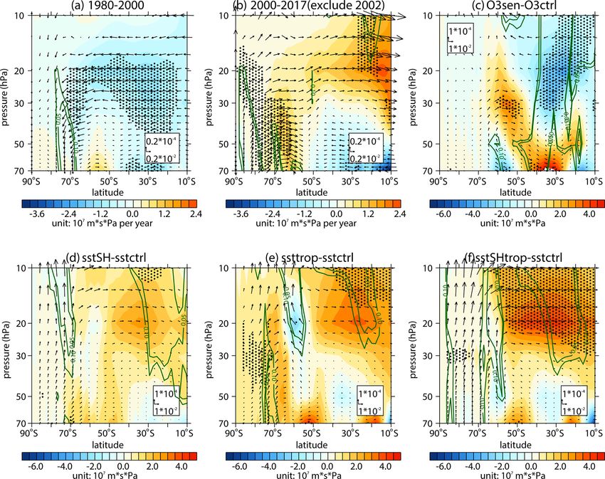
1580                       Y. Hu et al.: Weakening of Antarctic stratospheric planetary wave activities since the early 2000s

Table 1. Configurations of experiments for SST trends.

       Experiments    Descriptions
       sstctrl        Control run, where the seasonal cycle of monthly mean global SST data over 1980–2000 are derived from the
                      ERSST v5 dataset. Fixed values of ozone greenhouse gases and aerosol fields in the year 2000 are used.
       sstNH          As in sstctrl but with linear increments of SST in September over 2000–2017 in the NH (20–70◦ N). The applied
                      global SST anomalies are shown in Fig. 7a.
       sstSH          As in sstctrl but with linear increments of SST in September over 2000–2017 in SH (20–70◦ S). The applied
                      global SST anomalies are shown in Fig. 7b.
       ssttrop        As in sstctrl but with linear increments of SST in September over 2000–2017 in the tropics (20◦ S–20◦ N). The
                      applied global SST anomalies are shown in Fig. 7c.
       sstSHtrop      As in sstctrl but with linear increments of SST in September over 2000–2017 in SHtrop (20◦ N–70◦ S). The
                      applied global SST anomalies are shown in Fig. 7d.

Table 2. Configurations of experiments for the ozone recovery trend.

       Experiments    Descriptions
       O3ctrl         Control run, where the seasonal cycle of monthly averaged global SST data over 1980–2000 are derived from
                      the ERSST v5 dataset. The seasonal cycle of monthly mean three-dimensional global ozone over 1980–2000 is
                      derived from the MERRA-2 dataset. The GHGs and aerosol fields are specified to be fixed values in the year
                      2000.
       O3sen          As in O3ctrl but superposed with linear increments of global ozone in September over 2001–2017. The ozone
                      data in 2002 are removed when the linear increments are calculated. The applied ozone anomalies in the SH are
                      shown in Fig. 5.

4   Response of Antarctic stratospheric wave activity                  ify that the ozone recovery is responsible for the weakening
    to ozone recovery                                                  of stratospheric wave activity. The role of ozone recovery in
                                                                       stratospheric wave changes needs to be further explored by
Previous studies have suggested that ozone depletion and               model simulations. In this section, we use a group of time
recovery are important to the climate shift that occurred              slice experiments (O3ctrl and O3sen) to address this issue.
around the year 2000 in the Southern Hemisphere during aus-               Figure 4 shows the time series and piecewise trends of
tral summer (e.g., Son et al., 2008; Thompson et al., 2011;            the September TCO in the Antarctic during 1980–2017. As
Barnes et al., 2014; Banerjee et al., 2020). The impacts of            reported by previous studies (e.g., Angell and Free, 2009;
stratospheric ozone changes on Antarctic wave propagation              Banerjee et al., 2020; Krzyścin, 2012; Solomon et al., 2016;
during austral summer has also been examined in previous               WMO, 2011; Zhang et al., 2014), the Antarctic ozone show
studies (e.g., Hu et al., 2015). However, whether ozone re-            a significant decline during 1980–2000 (Fig. 4a, b, c) and
covery in September explains the weakening of stratospheric            a slight recovery during 2001–2017 (Fig. 4a, d, e). The re-
planetary waves during the same month remains unclear. The             covery trend is calculated with the data in 2002 removed be-
correlation between the detrended time series of the Septem-           cause the large poleward transport induced by SSW in 2002
ber Antarctic total column ozone (TCO) derived from SBUV               leads to extreme values of ozone (e.g., Solomon et al., 2016).
and stratospheric vertical wave flux (Fz) is 0.70 (p = 0.0011)         In addition, the correlation of TCO between the MERRA-
during 2000–2017. The increase in wave activity in the polar           2 and SBUV datasets is 0.61 (p = 4.5 × 10⁻⁵ ), suggesting
stratosphere causes heating effects and suppresses the for-            the changes of TCO derived from the reanalysis dataset, and
mation of PSCs and, hence, slows down the ozone deple-                 the observations have a good consistency. Thus, in order to
tion (e.g., Shen et al., 2020a). Therefore, the Antarctic ozone        obtain a three-dimensional structure of ozone changes, the
and stratospheric wave activity show a statistically significant       ozone data from MERRA-2 are used to make forcing fields
positive correlation. Theoretically, heating effects caused by         for CESM. As described in Sect. 2, a control experiment
ozone recovery in the Antarctic stratosphere may also de-              (O3ctrl) forced by climatological ozone and a sensitivity ex-
celerate the Antarctic stratospheric polar vortex and induce           periment forced by the linear increment of global ozone in
more waves to propagate into stratosphere (Andrews et al.,             September during 2001–2017 are conducted to explore the
1987; Holton, 2004). These preliminary analysis cannot ver-            impacts of ozone recovery. The pattern of ozone forcing

Atmos. Chem. Phys., 22, 1575–1600, 2022                                                  https://doi.org/10.5194/acp-22-1575-2022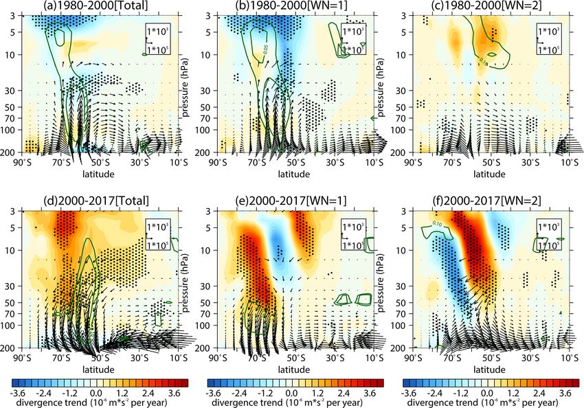
Y. Hu et al.: Weakening of Antarctic stratospheric planetary wave activities since the early 2000s                                   1581

Figure 1. Trends in the Southern Hemisphere (a, d) stratospheric E–P flux (arrows; units of horizontal and vertical components are 105 and
103 kg s−2 yr−1 , respectively) and its divergence (shading) with their (b, e) wave 1 components and (c, f) wave 2 components over (a, b,
c) 1980–2000 and (d, e, f) 2000–2017 in September, as derived from the MERRA-2 dataset. The stippled regions indicate the trend of the
E–P flux divergence significant at/above the 90 % confidence level. The green contours from outside to inside (corresponding to p = 0.1 and
0.05) indicate the trend of vertical E–P flux significant at the 90 % and 95 % confidence level, respectively.

Table 3. Correlations of stratospheric vertical wave flux time series (area weighted from 100 to 30 hPa over 70–50◦ S) between different
reanalysis dataset.

                                         ERA-Interim        JRA-55             MERRA-2            NCEP-2
                         ERA-Interim     1.00 (p = 0.00)    0.99 (p < 0.01)    0.98 (p < 0.01)    0.93 (p < 0.01)
                         JRA-55                             1.00 (p = 0.00)    0.98 (p < 0.01)    0.93 (p < 0.01)
                         MERRA-2                                               1.00 (p = 0.00)    0.94 (p < 0.01)
                         NCEP-2                                                                   1.00 (p = 0.00)

fields is similar to its trend patterns (Figs. 4d, e; 5a, b). Other     ery in the polar lower stratosphere absorbs more ultravio-
details of these two experiments have been given in Sect. 2             let radiation and causes cooling in the Antarctic troposphere
and Table 2.                                                            (Fig. 6b). To maintain the thermal balance, zonal wind accel-
   Figures 6 and 7 show the responses of the wave activ-                erates below 200 hPa over 60–70◦ S (Fig. 6a).
ity and wave propagation environment forced by O3sen.                      The changes in the zonal wind and temperature forced by
Note that the significant ozone recovery over the South                 the ozone recovery induce changes in the wave propagation
Pole mainly appears in the lower stratosphere (about 200                environment. The refractive index (RI) is a good matric to
to 50 hPa; Fig. 4e). In most southern polar regions, from               reflect the atmosphere state for wave propagation. Theoret-
50 to 3 hPa, the ozone recovery is not significant (Fig. 4e).           ically, planetary waves tend to propagate into large RI re-
The features are attributed to limitation of the emission of            gions (Andrews et al., 1987). The responses of RI and its
ozone-depleting substances (ODSs) and the reduction in het-             terms are shown in Fig. 6c–f. Note that the second term of RI
erogeneous reactions on PSCs, which mainly distribute in                does not change with atmospheric state, and the third term
the lower stratosphere (e.g., Solomon, 1999). Ozone recov-              of RI is insignificant compared to the first term (Hu et al.,

https://doi.org/10.5194/acp-22-1575-2022                                                 Atmos. Chem. Phys., 22, 1575–1600, 2022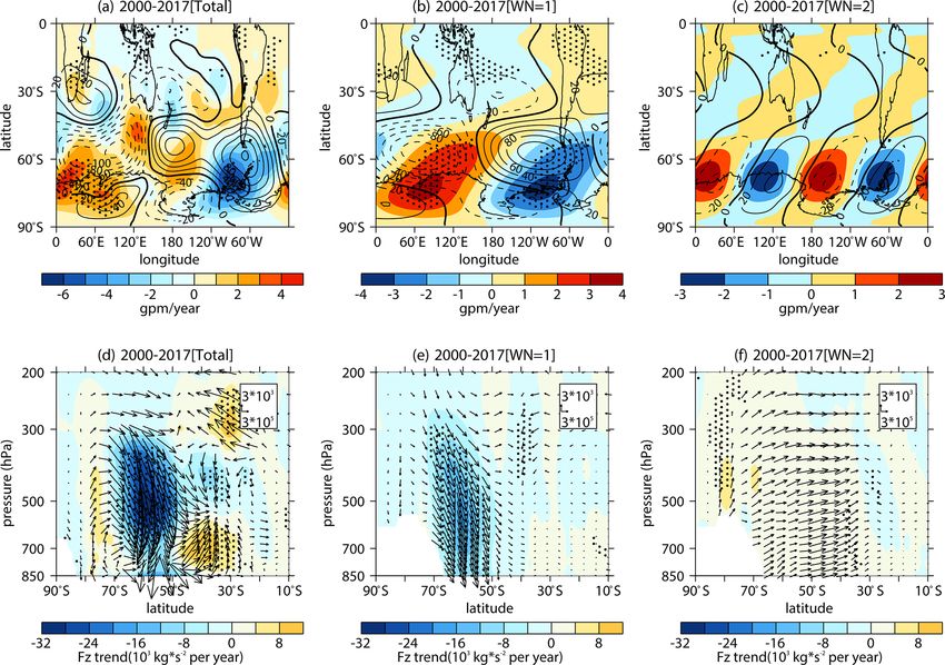
1582                         Y. Hu et al.: Weakening of Antarctic stratospheric planetary wave activities since the early 2000s

Figure 2. (a) The mean time series (solid lines) and piecewise (during 1980–2000 and 2000–2018) linear regressions (dashed lines) of
vertical E–P flux area weighted from 100 to 30 hPa over 70–50◦ S in September during 1980–2018 as derived from ERA-Interim (yellow),
MERRA-2 (blue), JRA-55 (red), and NCEP-2 (green). Panel (b) is the same as panel (a), except that the data in 2002 are removed. (c, d, e,
f) The trends (dots) and uncertainties (error bars) calculated during various periods using the change point method with different beginning
and ending years (titles). Circles and squares in panels (c), (d), (e), and (f) represent positive trends from the beginning years to change
point years (x axes) and negative trends from change point years to ending years, respectively. Different colors of the dots and error bars in
panels (c), (d), (e), and (f) correspond to colors in panel (a), which represent trends and uncertainties derived from different datasets. The
long and short error bars in same color reflect the 95 % and 90 % confidence intervals calculated by two-tailed t test. The error bar is omitted
when the significance of the trend is lower than the corresponding confidence level. Negative trends and corresponding uncertainties with
the beginning change point in the years after 2005 are also omitted, since the trend value shows a large fluctuation with the shortening of the
time series. Panels (g), (h), (i), and (j) are the same as panels (c), (d), (e), and (f), except that the data in 2002 are removed when calculating
trends and uncertainties.

2019). Previous studies indicate that changes in zonal mean                 lar regions (Fig. 6c, d). According to the Eq. (5), the first
potential vorticity meridional gradient q̄ϕ could explain the               term of q̄ϕ does not change
                                                                                                      h with thei atmospheric state. There-
changes in RI in the middle and high latitudes (e.g., Hu et                                                (ū cos ϕ)ϕ
                                                                            fore, the second term (−                     ;
                                                                                                                  hereafter the uyy term
                                                                                                              cos ϕ
al., 2019; Simpson et al., 2009). Consistent with these stud-                                                          ϕ
                                                                                                                        2

ies, the pattern of q̄ϕ shows some similarity with pattern of               or barotropic term) and the third term (− fρ0 ρ0 Nūz2 ; here-
                                                                                                                                          z
RI (Fig. 6c, d), especially in lower stratosphere over subpo-

Atmos. Chem. Phys., 22, 1575–1600, 2022                                                        https://doi.org/10.5194/acp-22-1575-2022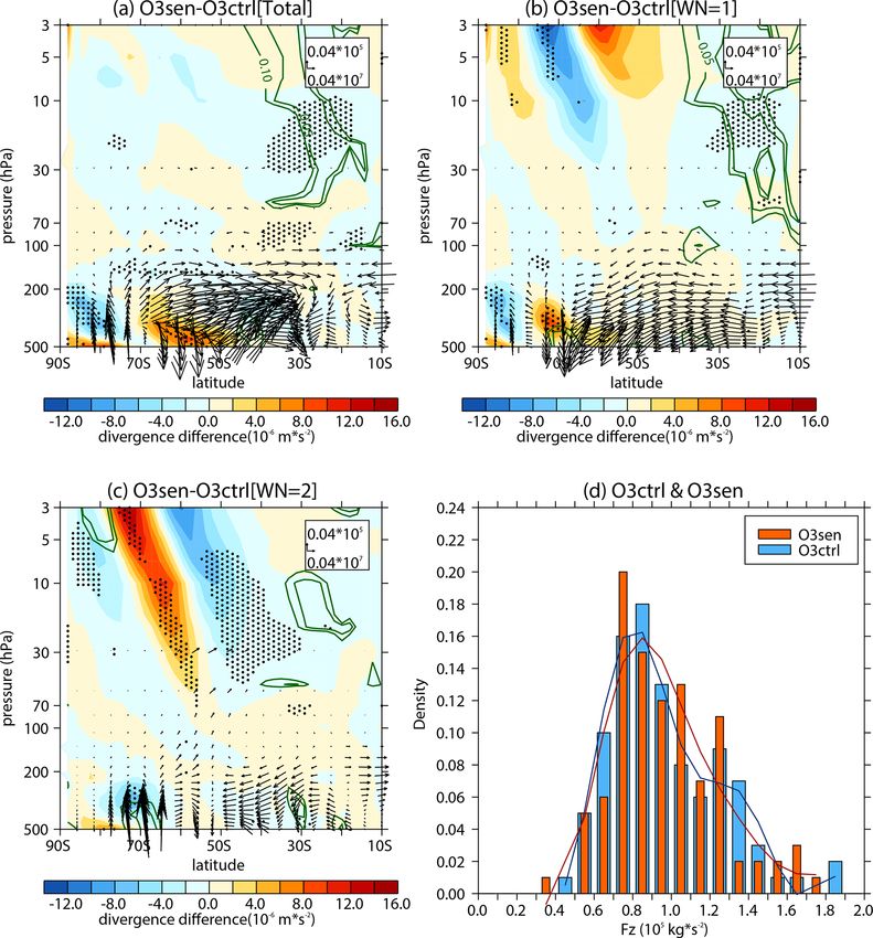
Y. Hu et al.: Weakening of Antarctic stratospheric planetary wave activities since the early 2000s 1583
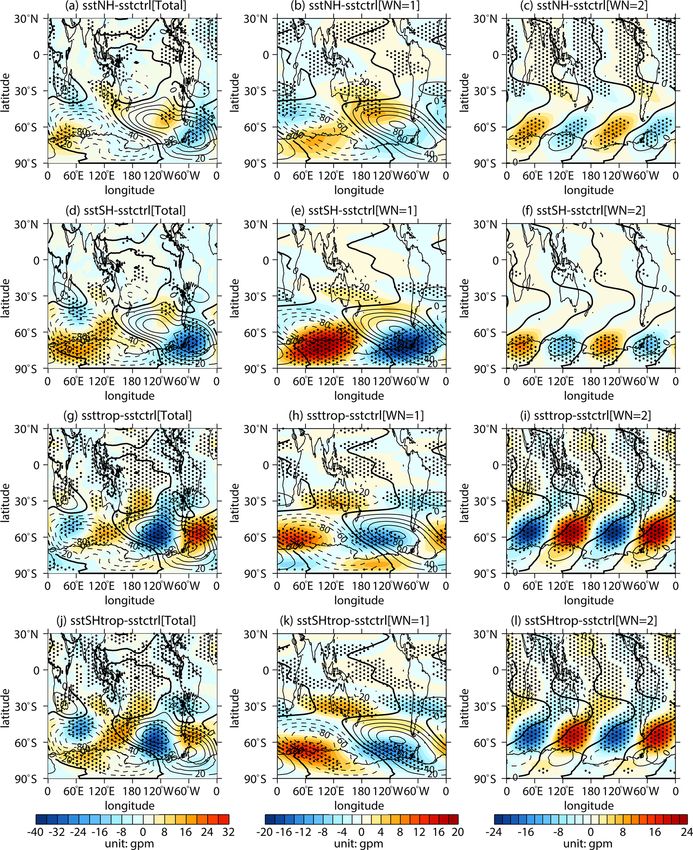
Figure 3. Trends (shading) and climatological distributions (contours with an interval of 20 gpm (geopotential meters); positive and negative
values are depicted by solid and dashed lines, respectively; zeroes are depicted by thick solid lines) of southern hemispheric (a) 500 hPa
geopotential height zonal deviations, with their (b) wave 1 component and (c) wave 2 component in September during 2000–2017, as
derived from the MERRA-2 dataset. Trends of the southern hemispheric (d) tropospheric E–P flux (arrows; units of horizontal and vertical
components are 3 × 10⁵ and 3 × 10³ kg s−2 yr−1 , respectively) and its vertical component (shading), with their (e) wave 1 component and
(f) wave 2 component in September during 2000–2017, as derived from the MERRA-2 dataset. The stippled regions represent the trend
significant at/above the 90 % confidence level.
after the uzz term or baroclinic term) are investigated. Note troposphere and lower stratosphere to some extent. However,
that the pattern of responses in the baroclinic term is simi- these weak responses still cannot explain the significant de-
lar with q̄ϕ (Fig.6d, f). The uzz term also can be written as crease of stratospheric wave flux in September.
f2 2 2
2
f dN f
HN2
+N 4 dz ūz − N 2 ūzz . Meanwhile, zonal wind accel-
eration in the upper troposphere weakens the vertical shear 5 Role of SST trends in the weakening of Antarctic
of u (ūz ) around 200 hPa over subpolar regions, inducing a stratospheric wave activities
decrease in the baroclinic term and RI in upper troposphere
and lower stratosphere (UTLS) over 60–70◦ S (Fig. 6d, f). In this section, we further explore the factors responsible
The response of RI induces a slight decrease in the vertical for the weakening of tropospheric wave sources and strato-
wave flux in UTLS over subpolar regions (Fig. 7a), which is spheric wave activities since the early 2000s in early aus-
mainly contributed by its wave 1 component (Fig. 7b). How- tral spring. Many studies reported that SST variations can
ever, the changes in the wave activity in UTLS are not signif- affect stratospheric climate (e.g., Li, 2009; Hurwitz et al.,
icant in the ensemble mean of the simulations (Fig. 7a, b, c). 2011; Lin et al., 2012; Hu et al., 2014, 2018; Tian et al.,
Meanwhile, note that the responses of zonal wind and tem- 2017; Xie et al., 2020). Hu and Fu (2009) also attributed
perature to ozone recovery are not significant above 50 hPa the strengthened stratospheric wave activities in the South-
over subpolar regions (Fig. 6a, b), thus inducing negligible ern Hemisphere to the SST trend from the early 1980s to
changes in the wave propagation environment (Fig. 6c) and the early 2000s. Furthermore, global SST in September dur-
wave activity (Fig. 7) in the middle and upper stratosphere. ing 2000–2017 also has a significant trend. The significant
In a word, the significant ozone recovery in the Antarc- warming pattern is mainly found over the southern Indian
tic lower stratosphere changes the wave propagation in upper ocean, the southern Atlantic ocean, the eastern and western
https://doi.org/10.5194/acp-22-1575-2022 Atmos. Chem. Phys., 22, 1575–1600, 2022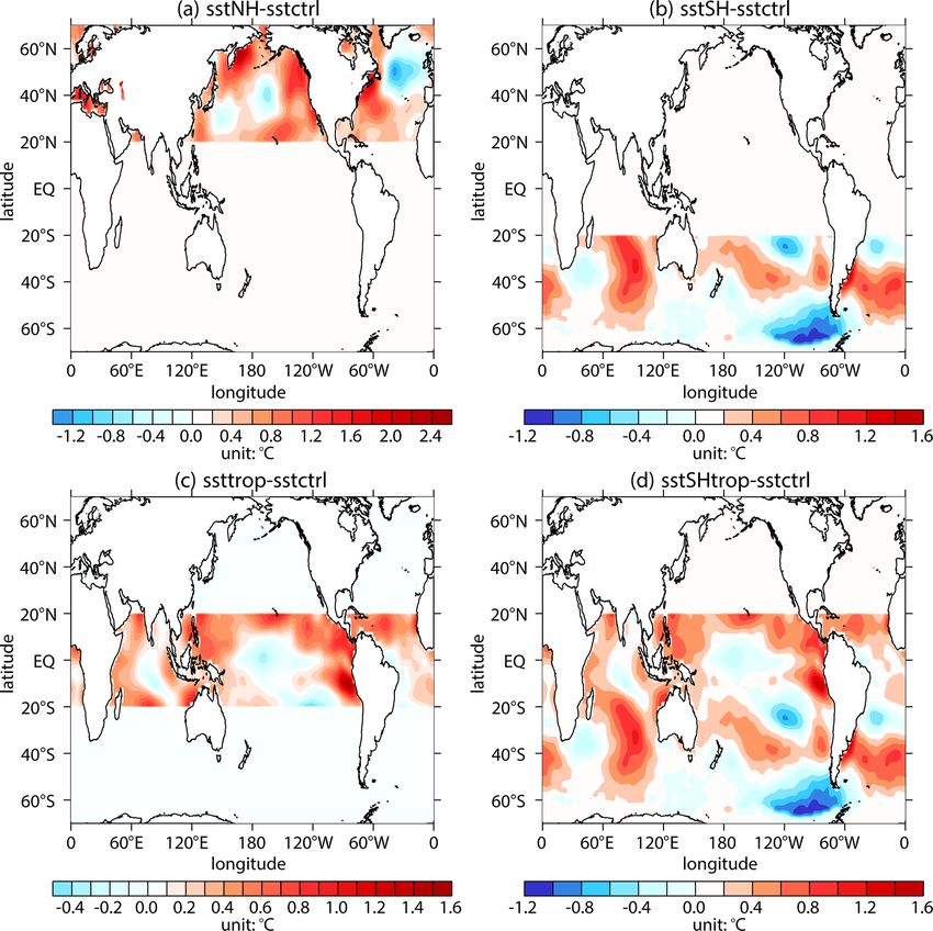
1584                       Y. Hu et al.: Weakening of Antarctic stratospheric planetary wave activities since the early 2000s

Figure 4. (a) Time series (solid lines) of area-weighted total column ozone (TCO) over 60 to 90◦ S as derived from the MERRA-2 (red) and
SBUV (blue) datasets. The dashed lines represent linear regression of TCO. (b, d) The TCO trends in September during 1980–2000 (b) and
2001–2017 (d) as derived from the MERRA-2 dataset. The outermost latitudes in panels (c, d) are both 40◦ S. (c, e) The zonal mean ozone
trends on the latitude pressure profile in September during 1980–2000 (c) and 2001–2017 (e) as derived from the MERRA-2 dataset. The
stippled regions in panels (b)–(e) represent trends significant at/above the 90 % confidence level. Data from 2002 are removed when trends,
regressions, and significances are calculated in this figure.

equatorial Pacific, and the western equatorial and northern             an insignificant trend during 1980–2000 and a significant
Atlantic ocean (Fig. 8b). A significant cooling pattern is lo-          warming trend during 2000–2017 (Fig. 8c). The subtropical
cated over the southeastern Pacific (Fig. 8b). In addition, the         Pacific Ocean in east of Australia is linked with the Pacific–
transitions around the year 2000 exist in the SST time series           South American (PSA) wave train (e.g., Shen et al., 2020b),
over some regions. In the southern Indian ocean, SST shows              and the SST there shows a significant warming trend during

Atmos. Chem. Phys., 22, 1575–1600, 2022                                                   https://doi.org/10.5194/acp-22-1575-2022
Y. Hu et al.: Weakening of Antarctic stratospheric planetary wave activities since the early 2000s                                    1585

Figure 5. (a) Difference in the horizontal ozone forcing field averaged from 1000 to 1 hPa between O3sen and O3ctrl. The outermost latitude
in panel (a) is 40◦ S. (b) Zonal mean difference in the ozone forcing fields on latitude pressure profile in the Southern Hemisphere between
O3sen and O3ctrl.

1980–2000 and an insignificant trend during 2000–2017. The              the SHtrop region (Fig. 9j), indicating that the connection be-
SST in the southeastern Pacific shows an insignificant trend            tween SST trends in the extratropical Northern Hemisphere
during 1980–2000 and significant cooling during 2000–2017               and the trend of stratospheric wave activity is weak.
(Fig. 8e). Trends of SST in southern Atlantic Ocean are the                Figure 10 shows the first three EOF modes of the Septem-
opposite during these two piecewise periods, showing sig-               ber SST in the SHtrop region during 2000–2017. The sec-
nificant cooling during 1980–2000 and significant warming               ond mode (Fig. 10b) shows a great similarity to the spatial
during 2000–2017. It is apparent that the spatial pattern of            pattern of the SST trend (Fig. 8b), and the corresponding
SST trend during 2000–2017 is obviously different from that             PC2 time series also has a significant trend (slope = 1.71;
during 1980–2000 (Fig. 8a, b), which may affect the tropo-              p < 0.01). The correlation between PC2 and Fz is signifi-
spheric wave sources. Thus, it is necessary to analyze the              cant (r = −0.56; p = 0.016), and the correlation coefficient
connection between SST trend and wave activity trend since              remains significant (r = −0.46; p = 0.065) at the 90 % con-
the early 2000s.                                                        fidence level when the value in 2002 is removed. This result
   Figure 9 shows the significance of the trend of the prin-            suggests that the SST trend in the SHtrop region is closely
ciple component (PC) time series of the SST in different                related to the recent weakening of the stratospheric wave ac-
regions (Fig. 9a–f) and the significance of the correlations            tivities. The first EOF mode is similar to IPO (Fig. 10a), and
(Fig. 9g–l) between the PC time series and Fz in September              its corresponding principal component is significantly corre-
during various periods. The trend of the PC1 time series in             lated (r = −0.98; p < 0.01) with the unfiltered IPO index.
the SH region is significant during serval periods (Fig. 9a),           However, it shows no significant trend (Fig. 10d) and has no
while the correlation between PC1 and Fz is only significant            significant correlation (Fig. 10g) with the stratospheric wave
with the particular ending year of 2015 (Fig. 9g). This fea-            flux, implying that the link between the IPO phase change
ture suggests that the connection between the SST trend in              at around the year 2000 (e.g., Trenberth and Fasullo, 2013)
SH region and the trend of stratospheric wave activity is not           and the weakening of Antarctic stratospheric wave activities
robust. The correlation between trend of stratospheric wave             is weak. The correlation between PC3 and Fz is also not sig-
activity and that of SST in the TROP or NH regions is also              nificant (Fig. 10i). Therefore, it is possible that the combined
weak (Fig. 9e, f). As for the combined regions, note that the           effect of the SST trend (the second EOF mode) in the tropical
PC2 time series in the SHtrop region has a significant trend            and extratropical Southern Hemisphere has led to the weak-
(Fig. 9d), and the correlation between the PC2 time series in           ening of stratospheric wave activities in early austral spring
SHtrop and Fz with the beginning year of around the year                since the early 2000s.
2000 is also significant (Fig. 9j), regardless of the differ-
ent ending years. This feature implies that the extratropical
Southern Hemisphere and tropical SST has a robust connec-               6   Simulated changes in Antarctic stratospheric
tion with stratospheric wave activities in early austral spring             wave activities forced by SST trends
since the early 2000s. The correlations between Fz and all PC
time series in the NHtrop (Fig. 9k) and globe (Fig. 9l) regions         The analysis in Sect. 5 suggests that the SST changes in the
are not as robust as those between Fz and PC2 time series in            SHtrop region may contribute to the weakening of the south-
                                                                        ern hemispheric stratospheric wave activities. Here, numeri-

https://doi.org/10.5194/acp-22-1575-2022                                                 Atmos. Chem. Phys., 22, 1575–1600, 2022
1586 Y. Hu et al.: Weakening of Antarctic stratospheric planetary wave activities since the early 2000s
Figure 6. Differences in the (a) zonally averaged zonal wind, (b) zonally averaged temperature, (c) refractive index, (d) a 2 q̄ϕ ,
h
(ū cos ϕ)
i 2 2
(e) − cos ϕ ϕ (uyy term), and (f) − a ρf0 ρ0 ūz2 (uzz term) between O3sen and O3ctrl. The stippled regions represent the differ-
ϕ N z
ence significant at/above 90 % confidence level.
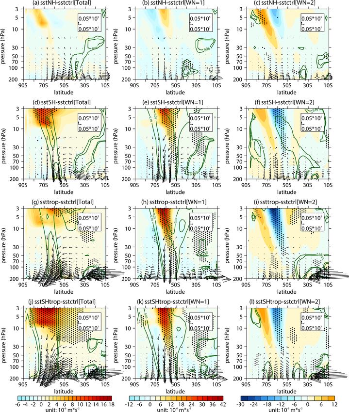
Atmos. Chem. Phys., 22, 1575–1600, 2022 https://doi.org/10.5194/acp-22-1575-2022Y. Hu et al.: Weakening of Antarctic stratospheric planetary wave activities since the early 2000s 1587 Figure 7. Differences in the (a) stratospheric E–P flux (arrows; units in horizontal and vertical components are 0.04 × 10⁷ and 0.04 × 10⁵ kg s−2 , respectively) and its divergence (shading) with their (b) wave 1 component and (c) wave 2 component between the sensitivity experiment (O3sen) and the control experiment (O3ctrl). The stippled regions represent the mean differences in the E–P flux divergence significant at/above the 90 % confidence level. The green contours from outside to inside (corresponding to p = 0.1 and 0.05) represent the mean differences in the vertical E–P flux significant at the 90 % and 95 % confidence levels, respectively. (d) Frequency dis- tributions (pillars; blue for O3ctrl and orange for O3sen) of vertical E–P flux (Fz; area weighted from 200 to 10 hPa over 70–50◦ S) and its five-point low-pass filtered fitting curves (solid lines; blue for O3ctrl and red for O3sen) derived from 100 ensemble members. cal experiments sstNH, sstSH, ssttrop, and sstSHtrop, forced pose on the corresponding climatological patterns in an out- by linear increments of SST in September during 2000–2017 of-phase style (Fig. 12e, f, h, i, k, l), indicating that the (Fig. 11; more details can be found in Sect. 2), are conducted changes in SST in SH, TROP, and SHtrop lead to a weaken- to verify the results presented in Sect. 5. ing of tropospheric wave sources in the extratropical South- Figure 12 shows the simulated response of 500 hPa geopo- ern Hemisphere. However, the predominate wave 1 compo- tential height to SST changes in different regions. The clima- nent of the 500 hPa geopotential height anomaly in the ex- tological distributions of the wave 1 component (Fig. 12b, e, tratropical Southern Hemisphere forced by the experiment h, k) and the wave 2 component (Fig. 12c, f, i, l) from the with NH SST change is relatively weak (Fig. 12b). This fea- simulations are consistent with that from reanalysis dataset ture suggests that the SST changes in extratropical North- (Fig. 3b, c), indicating that the model can capture spatial ern Hemisphere are incapable of inducing a robust response distributions of the atmospheric waves well. Note that the of tropospheric wave sources in the extratropical Southern wave 1 and wave 2 anomalies simulated with SST changes Hemisphere. in SH, TROP, and SHtrop are all significant. They super- https://doi.org/10.5194/acp-22-1575-2022 Atmos. Chem. Phys., 22, 1575–1600, 2022
1588                        Y. Hu et al.: Weakening of Antarctic stratospheric planetary wave activities since the early 2000s

Figure 8. Trends of SST in September over (a) 1980–2000 and (b) 2000–2017 as derived from the ERSST v5 dataset. The stippled regions
represent the trends significant at/above the 90 % confidence level. (c–f) Time series (blue solid lines) of SST during 1980–2017 over different
regions (titles). The dashed lines represent linear regressions of the SST time series on piecewise periods (1980–2000 and 2000–2017). The
labels of trend1 and trend2 in panels (c)–(f) represent the trend coefficients and the corresponding significances (in parentheses) over 1980–
2000 and 2000–2017, respectively.

  Figure 13 shows the simulated responses of stratospheric                are mainly attributed to the responses of the wave 1 compo-
wave activities in the Southern Hemisphere to SST changes                 nent (Fig. 13e, h, k). These results are consistent with the
over different regions. It is apparent that the experiments with          responses of tropospheric wave sources (Fig. 12d, e, g, h,
SST changes in SH, TROP, and SHtrop show significantly                    j, k). However, there are no significant anomalies of strato-
weakened stratospheric wave activities (Fig. 13d, g, j), which            spheric wave flux in the subpolar region in Fig. 13a and b,

Atmos. Chem. Phys., 22, 1575–1600, 2022                                                       https://doi.org/10.5194/acp-22-1575-2022
Y. Hu et al.: Weakening of Antarctic stratospheric planetary wave activities since the early 2000s                                           1589

Figure 9. Trend significance of the first three SST principal components (PCs) in (a) the extratropical Southern Hemisphere (SH; 70–20◦ S),
(b) the tropics (TROP; 20◦ S–20◦ N), (c) the extratropical Northern Hemisphere (NH; 20–70◦ N), (d) the extratropical Southern Hemisphere
and the tropics (SHtrop; 70◦ S–20◦ N), (e) the extratropical Northern Hemisphere and the tropics (NHtrop; 20◦ S–70◦ N), (f) the globe
(70◦ S–70◦ N), and the corresponding (g, h, i, j, k, l) correlation significances between them and the vertical E–P flux (Fz; area weighted
from 100 to 30 hPa over 70–50◦ S) during different beginning years (x axes) and ending years (y axes). The red and blue dots indicate
that a positive and negative trend or correlation coefficient are significant, respectively. The black dots indicate that the trends or correlation
coefficients are not significant. The stars indicate that the trends and the corresponding correlation coefficients are both significant. Each panel
is divided into three regions, from bottom to top, corresponding to the first, second, and third PCs, respectively. The criterion to distinguish
whether the trends and correlations are significant or not is the 90 % confidence level.

which is consistent with the response of corresponding tro-                 in Fig. 14b, c and d, suggesting that the SST changes in
pospheric wave sources (Fig. 12a, b) and the weak correla-                  SH, TROP, and SHtrop regions weaken the upward propa-
tion between Fz and the PC time series of SST in NH region                  gation of stratospheric wave flux. The area-weighted anoma-
(Fig. 9i). The result here suggests that the response of South-             lies of vertical E–P flux in the subpolar region of the South-
ern Hemisphere stratospheric wave activities to SST trend in                ern Hemisphere, induced by SST changes in SH, TROP,
NH region is weak.                                                          and SHtrop regions, are −0.084 × 10⁵ , −0.12 × 10⁵ , and
    The results of stratospheric vertical wave flux over 50–                −0.13 × 10⁵ kg s−2 , respectively. The sum of the anomalies
70◦ S derived from the 100 ensemble members of each ex-                     forced by sstSH and ssttrop is not equal to the anomaly
periment are shown in Fig. S4, and the frequency distribu-                  forced by sstSHtrop, which may result from nonlinear in-
tions of them are displayed in Fig. 14. Compared to the blue                teractions between the responses of wave activities to SST
fitting curves, the red fitting curves shift to the left, as shown          trends in SH region and TROP region. The weakening of

https://doi.org/10.5194/acp-22-1575-2022                                                      Atmos. Chem. Phys., 22, 1575–1600, 2022
1590 Y. Hu et al.: Weakening of Antarctic stratospheric planetary wave activities since the early 2000s Figure 10. (a, b, c) The first three EOF patterns of SST in the SHtrop region. (d, e, f) The original time series of the first three principle components (PCs; blue solid lines correspond to left inverted y axes) and stratospheric vertical E–P flux (Fz; area weighted from 100 to 30 hPa over 70–50◦ S; red solid lines correspond to right y axes) in September during 2000–2017. The blue and red dashed lines in panels (d), (e), and (f) represent the linear regressions of PC time series and Fz time series, respectively. The meaning of panels (g), (h), and (i) is the same as panels (d), (e), and (f), correspondingly, except for the detrended time series. The numbers without (and in) parentheses in panels (g), (h), and (i) represent the correlation coefficients between the detrended PC time series and Fz time series and the corresponding p values calculated by the two-tailed t test, respectively. stratospheric wave activities forced by SST increment in the ern Hemisphere. It also explains why the independent corre- tropical region is more significant than that in extratropical lation between Fz and PC time series obtained over SH or Southern Hemisphere (Fig. 14b, c, e), implying that the SST TROP region is not as significant as that between Fz and PC trend in the tropical region has contributed more to the weak- time series obtained over the SHtrop region (Fig. 9g, h, j). ening of stratospheric wave activities since the year 2000. Moreover, the mean linear increment of area-weighted verti- Meanwhile, it is apparent that the weakening of the South- cal E–P flux from 200 to 10 hPa over 70–50◦ S in September ern Hemisphere stratospheric wave activities forced by sst- during 2000–2017, as derived from four reanalysis datasets, SHtrop is the most significant among all the sensitivity exper- is about −0.38 × 10⁵ kg s−2 . Therefore, the contribution of iments (Fig. 14e). The reduction in the vertical E–P flux over the SST trend over 20◦ N–70◦ S (the SHtrop region) to the 50–70◦ S (200–10 hPa) forced by sstSHtrop is approximately weakening of stratospheric activities is approximately 34 %. 12 %. These modeling results indicate that the weakening of In addition, the reanalysis datasets show that the Brewer– the Antarctic stratospheric wave activities in September since Dobson circulation related to wave activities in the strato- the year 2000 has been induced mainly by the combined ef- sphere weakened significantly in early austral spring during fects of SST trends in the tropical and extratropical South- 2000–2017 (Fig. 15b), which is contrary to the intensified Atmos. Chem. Phys., 22, 1575–1600, 2022 https://doi.org/10.5194/acp-22-1575-2022
Y. Hu et al.: Weakening of Antarctic stratospheric planetary wave activities since the early 2000s                                  1591

Figure 11. Differences in the SST forcing field between sensitivity experiments (a sstNH; b sstSH; c ssttrop; d sstSHtrop) and the control
experiment (sstctrl).

trend during 1980–2000 (Fig. 15a). The transition of BDC               September (detailed evidence to address this issue is shown
around the year 2000 is believed to be associated with ozone           in the Appendix).
depletion and recovery (e.g., Polvani et al., 2017, 2018).
However, our modeling results suggest that the SST trend
has been responsible for the weakening of BDC in Septem-               7   Conclusions and discussions
ber since the year 2000 (Fig. 15d, e, f), The response of BDC
to ozone recovery is not significant (Fig. 15c) in September,          This study has analyzed the trend of Antarctic stratospheric
especially for the branch near the Antarctic. These results in-        planetary wave activities in early austral spring since the
dicate that, apart from the ozone depletion and recovery, the          early 2000s, based on various reanalysis datasets and model
SST trend should also be taken into consideration when ex-             simulations. Using the change point method, we find that
ploring the mechanism for the climate transition in the south-         the Antarctic stratospheric wave activities in September have
ern hemispheric stratosphere around the year 2000.                     been weakening significantly since the year 2000, which
   Previous studies reported that there is usually a time lag for      means the intensified trend of wave activities noted in previ-
tropic SST to affect extratropical circulation (e.g., Shaman           ous research (Hu and Fu, 2009; Lin et al., 2009) are reversed
and Tziperman, 2011). Thus, the impact of tropical SST                 after the year 2000 in early austral spring. Further analy-
change before September needs to be further examined. Our              sis suggests that the weakening of stratospheric wave activi-
simulations indicate that the tropical SST trend in Septem-            ties is related to the weakening of tropospheric wave sources
ber plays a dominate role in weakening of stratospheric wave           in extratropical Southern Hemisphere, which is mainly con-
activity at the same month, and the effect of tropical SST             tributed by the wave 1 component.
change before September is negligible compared to that in                 As the Antarctic ozone also shows clear shift around the
                                                                       year 2000, we firstly examine the impact of ozone recovery

https://doi.org/10.5194/acp-22-1575-2022                                                Atmos. Chem. Phys., 22, 1575–1600, 2022
You can also read