Using Sequence-Approximation Optimization and Radial-Basis-Function Network for Brake-Pedal Multi-Target Warping and Cooling

Article

Using Sequence-Approximation Optimization and
Radial-Basis-Function Network for Brake-Pedal
Multi-Target Warping and Cooling
Hanjui Chang 1,2,*, Guangyi Zhang 1,2, Yue Sun 1,2 and Shuzhou Lu 1,2

 1 Department of Mechanical Engineering, College of Engineering, Shantou University,
 Shantou 515063, China; 20gyzhang1@stu.edu.cn (G.Z.); suny09222022@163.com (Y.S.);
 21szlu@stu.edu.cn (S.L.)
 2 Intelligent Manufacturing Key Laboratory of Ministry of Education, Shantou University,

 Shantou 515063, China
 * Correspondence: changhj@stu.edu.cn

 Abstract: This paper uses a multi-objective optimization method to optimize the injection-molding
 defects of automotive pedals. Compared with the traditional automotive pedal material, aluminum
 alloy, the polymer pedal containing glass fibers not only reduces the aluminum pedal by at least
 half, but also improves the strength and hardness of the fibers by adjusting the orientation of the
 fibers in all directions. Injection factors include: filling time, filling pressure, melt temperature, cool-
 ing time, injection time, etc. For the optimization process influencing factors, herein, we focus on
 warpage analyzed via flow simulation, and setting warpage parameters and cycle time as discussed
 by setting different cooling distributions, pressures and temperature schemes. The multi-objective
 optimization design was mainly used to describe the relationship between cycle time and warpage,
 and the Pareto boundary was used for cycle time and warpage to identify the deviation function
 and radial-basis-function network. We worked with a small DOE for building the surface to run
Citation: Chang, H.; Zhang, G.;
Sun, Y.; Lu, S. Using Sequence-
 SAO programming—which improved the accuracy of the response surface by adding sampling
Approximation Optimization and points—terminating the time when the warpage value met the solution requirements, to find out
Radial-Basis-Function Network for the global optimal solution of the warpage value under different cooling times. Finally, the results
Brake-Pedal Multi-Target Warping highlighted four influencing parameters that match the experimental image of the actual produc-
and Cooling. Polymers 2022, 14, 2578. tion.
https://doi.org/10.3390/
polym14132578 Keywords: warpage; cycle time; sequential approximate optimization; conformal cooling channel;
Academic Editor: Luigi Sorrentino
 Pareto boundary; brake pedal

Received: 20 May 2022
Accepted: 22 June 2022
Published: 25 June 2022
 1. Introduction
Publisher’s Note: MDPI stays neu- The molding conditions of the injection pedal can also affect the productivity, cycle
tral with regard to jurisdictional
 time and energy consumption of the molding process. The molding conditions of the in-
claims in published maps and institu-
 jection pedal are closely related to other factors that determine the quality of plastic prod-
tional affiliations.
 ucts, such as material, parts design, mold and other factors. The injection-molding factors
 studied in this experiment include: filling time, packing pressure, melt temperature, cool-
 ing time, injection time, etc.
 The quality of a molded part depends on the process parameters and the properties
Copyright: © 2022 by the authors. Li-
censee MDPI, Basel, Switzerland.
 of the plastic material. Finding the best process parameters can effectively reduce the
This article is an open access article
 number of cycles and improve product quality. The determination of process parameters
distributed under the terms and con- in the actual production largely depends on the experience of the plastic engineers and
ditions of the Creative Commons At- the actual site commissioning. This method does not effectively ensure the accuracy of the
tribution (CC BY) license (http://crea- process parameter values. With plastic it is difficult to predict thermal bonding properties,
tivecommons.org/licenses/by/4.0/). how to set the optimal molding conditions, and how to maximize the required product

Polymers 2022, 14, 2578. https://doi.org/10.3390/polym14132578 www.mdpi.com/journal/polymers

Polymers 2022, 14, 2578 2 of 23

 quality, which are crucial. Therefore, the process parameters are usually selected from the
 manual and then adjusted using the trial-and-error method. As can be seen, trial-and-
 error is expensive and time consuming. For manual lysis methods, many mathematical
 equations have been developed to derive the inherent process parameters for injection
 molding. However, when analytical equations involve many simplifications, they often
 do not meet the reliability requirement due to the complexity of the injection process. As
 a result, many researchers are trying to find ways to optimize the parameters of the mold-
 ing process.
 The production advantages of plastic products are light weight, high stiffness and
 high productivity. Therefore, compared with the commonly used all-aluminum pedal, the
 brake pedal in polymer materials will have the advantage of lighter weight and better
 strength. The three main stages of the widely used plastic injection-molding (PIM) [1] pro-
 cess are: the filling stage, pressure holding stage and cooling stage. First, during the filling
 stage, the molten plastic is filled into the cavity type of the mold under the pressure of the
 injection-molding machine. Secondly, in the holding stage, the molten plastic is com-
 pressed at very high pressure to obtain the shape of the part. The molten plastic solidifies
 during the cooling phase. The final cooling of the formed solid plastic is lifted out of the
 mechanism. Therefore, in order to improve the cycle time and warping time simultane-
 ously, it is necessary to optimize the melt temperature, pressure-retaining pressure, pres-
 sure fixation time, injection time, cooling time and other process parameters. In addition,
 deformation, volume shrinkage and welding line are the main defects that should be
 avoided for size accuracy and the appearance of the finished product, in order to obtain
 higher-quality products. The design function of the pedal is mainly to optimize the design
 of the cooling pipe and shorten the entire product-molding cycle, including filling, pres-
 sure, cooling, etc. Deformation and cooling shrinkage also need to be reduced, which can
 be further optimized by optimizing the design of the cooling pipe for better injection-
 molding parameters and product quality. In the design process of the conformal cooling
 waterway, it is necessary to continuously adjust the relevant parameters, such as the di-
 ameter of the cooling-water pipe, the number of cooling-water pipes, the arrangement of
 the cooling-water circuit, etc.; constantly adjust the parameters in combination with the
 warpage and cooling results of the simulation experiment; and finally, obtain the optimal
 cooling circuit design. This study optimizes the automotive automatic brake-pedal injec-
 tion-molding parameters and compares the original parameters with the optimized pa-
 rameter results; discusses the influence of these parameters on the product warpage
 shrinkage and molding cycle; and sets up different cooling channels, pressures and plastic
 temperature schemes.

 2. Literature Review
 In terms of reducing warpage deformation and obtaining optimal injection-molding
 parameters, this study requires multi-objective optimization, which is compared with
 other classical mathematical schemes in the following literature review process.
 In 2004, Mohd Sapuan Salit [1] analyzed and calculated the possible configurations
 and geometries of brake pedals. Based on the performance of existing and suitable poly-
 mer-matrix composites, the results show that polyamide with short glass fibers can be the
 most suitable material for polymer-based composite brake pedals. By properly designing
 the polymer-matrix brake pedals, one can reduce the weight by 73%. In 2006, Hassan Kur-
 taran and Tuncay Erzurumlu [2] used a combination of process parameters organized by
 experimental design, which were analyzed via statistical full three-level analysis. Accord-
 ing to the FEM results based on the analysis of variance (ANOVA) method, the most im-
 portant process parameter affecting warping was the within-mode pressure value. The
 response-surface model (RSM) with an effective genetic algorithm yielded the best pro-
 cess parameter value, with an optimization rate of 38%. In 2007, Y. C. Lam [3] proposed a
 strategy to optimize injection-molding conditions using a mixture of gradient methods
 and genetic algorithms, which first derived elite solutions from the genetic algorithm

Polymers 2022, 14, 2578 3 of 23

 optimization results to identify candidate local minimum regions. These solutions were
 searched as gradient methods for local minima from which the best solution was selected.
 The hybrid algorithm had more stable optimization results than single inheritance. In
 2007, Shen Changyu [4] proposed a method that combined artificial a neural network with
 a genetic algorithm to improve the quality index of part volume shrinkage change, estab-
 lished an neural network (NN) model of volume shrinkage change and process conditions
 of 5-9-1 structural injection molding, and verified the optimization results of genetic algo-
 rithm through numerical experiments. In 2008, Yuehua Gao [5] ordered SAO based on
 the Kriging model to minimize the warping of a phone case. The rectangular grid of the
 spatial filling sampling strategy of the Krieger model was modified using the functional
 relationship established by the Kriging model between warping and different parameters.
 The results show that the optimization method can effectively reduce warping.
 In general, population-based optimization techniques require a large number of func-
 tion evaluations to find the global minimum and a set of Pareto-optimal solutions. This
 makes it difficult to apply these optimization techniques directly to actual design optimi-
 zation issues in some cases due to time-consumption issues. Because classical mathemat-
 ical planning requires the sensitivity of goals and constraints, it is not suitable for non-
 micro-problems. In addition, a functional evaluation of sensitivity and step determination
 needs to be calculated. Today, the time available for developing new products is decreas-
 ing, so it is best to reduce the computational time required for optimization.
 In 2007, G. Gary Wang and S. Shan [6] summarized engineering design optimization
 using DOEs to set sample points in the design variable space, and evaluated the goals and
 constraints of these sample points via LHD. The response surface was constructed using
 a kriging and radial-basis-function (RBF) network, and finally the approximate optimal
 value was obtained by optimizing the response surface; this value was used as the ap-
 proximate optimization result. In 2009, Y. Zhang Y.M. Deng [7] proposed a method to
 reduce the warpage defects of injection parts. Mode-pursuing sampling (MPS) to warp
 optimization allowed more sample points to be systematically generated within the cur-
 rent optimal solution neighborhood while statistically covering the entire search space.
 The design variables for molding time, melt temperature and mold temperature showed
 that warpage deformation can be effectively reduced and the calculation results were sig-
 nificantly reduced. In 2009, in a study by Chuang Li and Fu-Li Wang [8], using a step-by-
 step optimization method based on an RBF proxy model, an advanced expected improve-
 ment criterion was proposed to improve the overall performance of the optimization
 method. Packaging contour optimization was applied to the injection-molding process to
 achieve shrinkage uniformity of molded parts. The improved approach enables stronger
 global optimization performance and more accurate optimal solutions without the need
 for appropriate padding data. In 2010, Yuehua Gao [9] proposed an adaptive optimization
 method based on the Kriging proxy model, and the adaptive process was implemented
 via the Expected Improvement (EI) fill sampling standard. The guide allows the use of
 DOEs for global searches in a very short period of time, and to find best design. The results
 showed that the adaptive multi-objective optimization method can effectively reduce the
 warpage of the mobile phone case. In 2011, Satoshi Kitayama [10] and others proposed a
 sequence-approximation optimization (SAO) algorithm based on the RBF network. A new
 adaptive scaling technology was developed; a new density function was constructed us-
 ing the RBF network to determine the sparse region between the sample points; the global
 minimum of the density function was used as the new sample point; and finally, the ap-
 proximate global optimal solution was obtained. In 2012, Kurtalan [11] obtained a local
 minimum value by scaling the method if the optimal value of the response face continued
 to increase. Global and local approximations are improved via sequential sampling strat-
 egies, and improved algorithms can be used to find sparse regions. In the EI algorithm,
 regions with high uncertainty correspond to sparse regions. In order to find the sparse
 regions, it is necessary to adjust the parameters in the Gaussian function. In 2013, Chul
 Woo Park [12] performed injection-molding analysis of truck pedals based on the location

Polymers 2022, 14, 2578 4 of 23

 of the gate. The runners were 5 mm and 100 mm high. There were four schemes: molding
 started from the round part of the brake-pedal shell, the brake shell with the straight part
 on both sides, the back of the brake case, and the part where the brake case was mounted
 on the body. Result had a minimum pressure of 30 Mpa.
 It is important to use global optimization techniques to find high-precision global
 minima, which often require a lot of function calculations. However, if the objectives and
 constraints are ambiguous, but can be evaluated via computationally intensive numerical
 simulations, the response surface (called metamodeling) is an attractive method for find-
 ing approximate global minima through a small amount of functional evaluation. Warp-
 ing deformation is a nonlinear implicit function of process conditions, usually solved us-
 ing finite-component (FE) equations, and the workload is very heavy. The Kriging model
 establishes an approximate function relationship between warping and process condi-
 tions, replacing the expensive warping reanalysis during optimization. The SAO method
 based on radial-basis-function network can meet the optimization requirements of injec-
 tion-molding process parameters.
 In 2014, Mohd Nizam Sudin [13] used CATIA V5 solid modeling software to generate
 a digital model of an existing brake pedal. Topology optimization under linear statical
 analysis was carried out using Altair OptiStruct software. A new lightweight brake-pedal
 design scheme was proposed. The results of the study showed that the newly designed
 brake pedal weighed 22% less than the existing brake pedal without sacrificing perfor-
 mance requirements. In 2014, Satoshi Kitayama [14] employed the SAO method using
 radial-basis-function networks. Taking the mold temperature and melt temperature as the
 design variables, short lenses of molten plastic that were not filled into the cavity were
 considered design constraints. The temperature distribution was analyzed, which showed
 that the variable pressure distribution could reduce the plastic temperature difference of
 the melt and effectively reduce warpage deformation. In 2014, Zhang [15] applied the
 kriging method to warpage and seal optimization through the pressure curve of
 shrinkage uniformity. They used a radial underlying function network to build
 the response surface. Additionally, in order to find undeveloped areas, they used
 the expected improvement function. The optimization rate of warpage results
 reached 28%. In 2014, Jian Zhao [16] proposed a two-stage multi-objective optimization
 framework based on Pareto-optimized injection-molding process parameters. The first
 phase used an IEGO algorithm to approximate the nonlinear relationship between ma-
 chining parameters and part-quality measurements. In the second phase, NSGA-II based
 on non-dominant sequencing was used to look for better convergence to the boundary of
 true Pareto. The double Pareto boundary indicated a significant relationship between
 warpage and volumetric shrinkage. In 2014, Wen-Chin Chen and Deni Kurniawan [17]
 used the Tamakou method, reverse propagation neural network (RPNN), genetic algo-
 rithm (GA), and particle group optimization in combination with a genetic algorithm
 (PSO-GA) to find the best parameter settings, and in the first phase of optimization, signal-
 to-noise ratio predictors and genetic algorithms were used to reduce the variance of mass
 characteristics. In the second stage of optimization, an S/N ratio predictor and mixed PSO-
 GA quality predictor were used to find the best parameter settings for process quality
 characteristics and stability, and the proposed system not only improved the quality of
 plastic parts, but also effectively reduced the variability of the process.
 It is important to note that the Tiankou method can find the best combination of pro-
 cess parameters, but the best process parameters cannot be found. Chen and Cunhawan
 recommend two-stage optimization using the Tiankou method and PSO-GA, wherein the
 Tiankou method is used to select the process parameters for the first stage, while the PSO-
 GA is used to determine the parameters for the second phase of the optimal process.
 Therefore, in order to obtain a high-precision response surface, it is often necessary to
 employ a large-scale experimental design. In recent years, the sequence-approximation
 optimization method has been widely used. In SAO, a small DOE is used first to build a
 response surface. One can then find the best value for the response face. The SAO

Polymers 2022, 14, 2578 5 of 23

 algorithm is terminated if the terminal criteria set by the designer are met. Note that the
 number of sampling points is equivalent to the number of simulated runs. In addition,
 some new sampling points are added to improve the accuracy of the response surface.
 Through the iterative process described above, a highly accurate global optimal solution
 can be found. Therefore, the orderly SAO of repeatedly building and optimizing response
 surfaces has become a common method for determining the best process parameters. In
 SAO, the response surface is repeatedly built and optimized by adding several new sam-
 pling points. One can then find a highly accurate global minimum. Doing this using re-
 sponse surfaces and neural networks is a “one-step” optimization set that does not require
 iteration. Build the response surface repeatedly by adding new sampling points until the
 final criteria set by the decision maker are met. Compared to the classic response-surface
 method described above, one can achieve high accuracy approximate to the lowest global
 value by adding new sampling points. However, when using SAO to obtain high-preci-
 sion data, it is often necessary to first consider the first target, which is to add the best
 point of the response face as the new sampling point. This results in high-precision local
 approximations. Adding new sampling points to sparse areas produces global approxi-
 mations. This addition prevents one from falling into the local minimum. SAO is used to
 identify Pareto boundaries with a small number of simulations.
 In general, the accompanying cooling channel improves cooling performance, cycle
 times and distortion. However, we do not know how to design subsequent cooling chan-
 nels. In other words, the design of the accompanying cooling channels depends, to a large
 extent, on the designer’s experience. In addition, redesigning cooling channels is expen-
 sive and difficult to try. Therefore, it is necessary to use single-target or multi-target opti-
 mization to obtain an optimally shaped cooling waterway. The first CAE simulation can
 display the performance output of conformal cooling channel (CCC) according to differ-
 ent targets such as cooling time, warping thickness, temperature distribution and thermal
 stress. By evaluating the resulting output, one can obtain more information about the im-
 pact of different CCC designs, but the simulation of the application may not be sufficient
 to obtain the best design conditions. Optimization is the step to determine the optimal
 design conditions for CCC.
 In 2010, Hong-Seok Park [18] proposed a conformal cooling channel with a bezel
 array, and a system of approximate equations was developed to represent the relationship
 between the cooling channel configuration, mold material, mold thickness, and tempera-
 ture distribution within a particular polymer. The appropriate physical mathematical
 model was established through experimental design, and the optimization process of ob-
 taining the target mold temperature and uniform temperature distribution and minimiz-
 ing cooling time was significantly improved. In 2014, Choi [19] implemented an advanced
 optimization method developed using a CCC, in which minimizing the average mold
 temperature of the cycle and obtaining temperature uniformity were the main goals of the
 study. The spacing (x), diameter (d), and distance (y) between the center of the groove and
 the cavity surface was preferred. The optimal operating condition parameter of the x-
 value was finally obtained, and the method can be widely used in the design of conformal
 waterways. In 2017, Hazwan MHM [20] simulated a slot-milled square CCC using a DOE
 full factorial design. After the application of regression models and ANOVA methods, the
 cooling time obtained was the factor that had the greatest impact on warp thickness. The
 results showed that the response-surface method was close to the improvement rate of the
 straight drilling channel and the CCC design in this study.
 In other words, the response-surface method can be used as the preferred method for
 improving and comparing research in both conventional and form-keeping cooling chan-
 nels. In addition, the results of the optimization of the straight drilling channel and square
 milling slot channel using the response-surface method and a genetic algorithm were
 compared. For the best warping thickness, optimization via genetic algorithm presented
 a slightly different optimization point to the response-surface method; therefore, it can be
 seen that both the response-surface method and the genetic algorithm can give similar

Polymers 2022, 14, 2578 6 of 23

 results to each other. From the brief review above, it is found that the best process param-
 eters can effectively reduce warping. Few papers focus on pressure curves, which have
 found that variable packaging pressure curves can also effectively reduce warping. How-
 ever, only the effectiveness of the packing pressure distribution is discussed. If injection
 pressure distribution is considered, warping will be reduced more effectively. Therefore,
 it is important and attractive to consider pressure distribution during the filling phase
 during powder-injection forming.
 Short shots of melt plastic that are not fully filled into the cavity are serious and fatal
 defects in PIM. Small injection pressure and lower mold temperatures can sometimes lead
 to short shots. To avoid short shots, the easiest way is to use high injection pressure and
 high mold temperature. Another way to avoid short shots is to use a high melting tem-
 perature.
 In 2017, Bikas [21] found the optimal gate thickness to minimize differences in filling
 time, combining neural networks with genetic algorithms (GA) to consider design
 variables in terms of mold temperature, melt temperature, injection time, and injection
 pressure. They approached the maximum shear stress by using a multilayer neural net-
 work, where warpage, volumetric shrinkage, and sink marks were considered objective
 functions. They used second-order polynomial response surfaces to approximate warpage
 and closure described in references. In 2018, Satoshi Kitayama [22] and others used a
 multi-objective optimization design for minimizing the soldering temperature by using
 the minimum clamping force, and the Pareto boundary between them was determined.
 They used the SAO of the radial-basis-function (RBF) network to identify Pareto bounda-
 ries. Numerical simulations clarified the equilibrium between the minimum welding tem-
 perature and the clamping force. In 2019, Hongwen He [23] proposed an accelerated-pe-
 dal single-foot regenerative braking control strategy based on an adaptive fuzzy control
 algorithm to effectively recover braking energy. Under the condition of secondary braking,
 a neural network controller of a composite braking system was proposed. The experi-
 mental results showed that the energy economy of IBS in three cycles was 3.67% higher
 than that of EU260, the braking severity was reduced, and the hydraulic braking time was
 2.27% lower than that of EU260.
 In 2019, Chen-Yuan Chung [24] combined finite element analysis with gradient-
 based algorithms and robust genetic algorithms to determine the optimal layout of cool-
 ing channels. The use of conformal cooling channels reduces surface temperature differ-
 ences, spray times and warpage of the melt. The fringe pattern is improved by the optimal
 values of melt temperature, mold temperature, filling time and package time obtained by
 experimental design, eliminating local variations of birefringence.
 In 2020, Chang [25] proposed a screw life prediction method based on a hybrid com-
 posite screw process-parameter method for dynamic iterative work. A combination of an
 automated virtual metering (VM) system and a recognizable performance evaluation
 (RPE) scheme was proposed. The injection of composite screws was predicted by extract-
 ing the characteristics of a given cutting condition and related process parameters from
 the sensor data. In 2020, Chang [26] proposed an optimization method based on the re-
 verse warpage model; this reduces the thermal conductivity of the plastic material and
 the curing layer on the mold surface, which means that the shrinkage of the melting zone
 in the component will continue to lead to warpage. The sensitivity of warpage prediction
 to the relationship between the two most important material properties (glass fiber and
 holding time) was analyzed. In 2020, Junren Shi [27] combined the driving data of experi-
 enced drivers in different driving environments with deep learning to build a deep long-
 term–short-term memory network to predict the aperture of the brake pedal under differ-
 ent braking types. The proposed anthropomorphic control method, which combines driv-
 ing data with deep learning, can be used to predict the aperture value of the pedal of the
 loading mechanism in a complex driving environment. The 2021 M.I.M. Sargini [28] study
 explored the possibility of rapidly producing brake pedals for metal cars using low-cost
 additive manufacturing techniques, using metallic polymer fiber filaments, followed by a

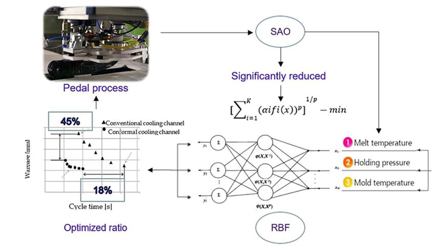
Polymers 2022, 14, 2578 7 of 23

 debonding and sintering process. Finite Element Analysis was applied to analyze the fea-
 sibility of a new brake pedal designed for AM machining. Physical tests were conducted
 on metal brake pedals produced by FDM, the results of the finite element analysis were
 verified, and the reliability of metal-based technology was evaluated.
 In 2021, Sai Li, Xi Ying Fan et al. [29] designed orthogonal experiments based on sim-
 ulation results while selecting important factors affecting warpage. The kriging model
 was established by using four related functions that affected the accuracy of the model,
 and the model was optimized using a numerical optimization algorithm, a direct search
 method and a global search method to obtain the best injection-molding parameters that
 produced the minimum warpage. In 2021, Shaochuan Feng et al. [30] conducted a system-
 atic evaluation of the design, manufacture and application of CC channels. They calcu-
 lated and selected some key design parameters for CC channels related to channel shape,
 size, and position, taking into account cooling performance, mechanical strength, and
 cooling hydraulic drops. By using CC channels for uniform and fast cooling, cycle times
 can be reduced by 70% and shape deviations can be significantly improved. In 2021, Yan-
 nik Lockner et al. [31] trained an artificial neural network based on transfer learning of
 induction networks to optimize the parameters of injection flow, packing time, packing
 pressure, cooling time, melt temperature and cavity wall temperature. Generating four
 sample points of the new process could train an injection-molding process model with a
 certainty (R2) of 0.9 or higher, compared to an 88% reduction in training data for the tra-
 ditional method. In 2021, Chil-Chyuan Kuo et al. [32] proposed a differential sensitivity-
 fusion method (DSFM), which used a metamodeling method to construct a response pre-
 dictor and calculate the target response of any sample point in the global design space.
 They obtained the Pareto-optimal solution, wherein the response-predicted value was
 used as the fitness function. Taking the front bumper of a car as an example, numerical
 results showed that the method had better prediction accuracy and performance.
 The cooling performance of the accompanying cooling channels was tested using
 digital and experimental methods. The cycle time and distortion of the brake pedal plastic
 were considered to be cooling properties, and the process parameters were optimized. In
 general, short cycles can cause large upturns, while long cycle times can cause small
 warps. Therefore, a trade-off between cycle time and warp was observed. The authors
 developed multi-objective design optimizations to determine trade-offs (Pareto Frontier).
 This study analyzes the modal flow simulation of pedals. The PA6 contains 40 types of
 fiberglass; it improves the cooling tube by comparing filling time, hold time, melting tem-
 perature, maximum cooling time, cooling to maximum temperature, etc., and will be fur-
 ther improved in the future. In addition, it is particularly important to shorten the process
 time, which is also beneficial to improve the production efficiency and economic efficiency
 of automobile products. Therefore, the design function is mainly to optimize the design
 of the cooling pipe, and to shorten the entire product-molding cycle, including filling,
 pressure, cooling, etc. There is also a need to reduce distortion and cooling shrinkage,
 which can be further optimized by optimizing the design of the cooling pipes; this can
 then be further optimized, for example, with better cooling effects. The purpose of this
 paper is to test the cooling performance of the accompanying cooling channels using dig-
 ital and experimental methods. The cycle time and distortion of the brake-pedal plastic
 are considered to be cooling properties, and the process parameters are optimized. In gen-
 eral, short cycles can cause large warpages, while long cycle times can lead to small warp-
 ages. Therefore, a trade-off between cycle time and warping is observed. We developed
 multi-objective design optimizations to determine trade-offs (Pareto Frontier). Numerical
 simulations are very dense, so the SAO in the radial-basis-function network developed by
 one of the authors was used to identify Pareto edge faces with a small amount of simula-
 tion. Based on the numerical results, the accompanying cooling channel was used for im-
 age analysis. The purpose of our study is to obtain an empirical curve that can be based
 on Pareto-optimal solutions, which can provide a reference for actual production and

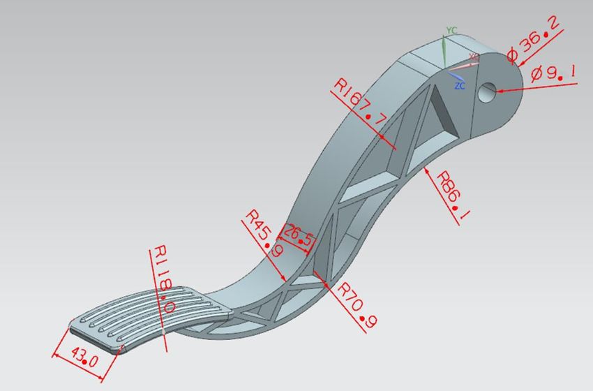
Polymers 2022, 14, 2578 8 of 23

 select appropriate Pareto-optimal solution points according to actual production needs.
 Listed below are five points detailing the main contributions:
 1. The response-surface method is used to identify the optimal arrangement of the cool-
 ing waterway, according to the cooling time, warping thickness, temperature distri-
 bution and thermal stress, and other different targets, to display the performance
 output of CCCs. The obtained output is evaluated.
 2. Because the relationship between target and constraint is not clear, the approximate
 global minimum value is found by means of computationally intensive numerical
 simulation and by using the method of response surface (called metamodeling).
 3. Multiple sampling points are set up in the design variable space. Orthogonal arrays
 or Latin designs (LHDs) are typically used to determine these sampling points. These
 sampling points are evaluated for targets and constraints.
 4. A response surface is constructed that approximates the target and constraint. Radial-
 basis-function (RBF) networks are used to construct response faces. Approximate op-
 timal values can be obtained by optimizing the response surface—both the response-
 surface optimization and the original design optimization problem of the order of the
 approximate optimization method (SAO).
 5. The SAO radial-base-network deviation function is used to identify the cycle time
 and warping in the Pareto boundary, to find a highly accurate global optimal solution
 to different cooling time warping values.

 3. Materials
 3.1. Product Introduction
 The experimental subject was a car pedal, with pedal size as shown in Figure 1; the
 pedal needs to withstand a large shear force and forward impact, so we choose the mate-
 rial with fiberglass (PA6 AKROMIDB B3 GF 40 schwarz (3383)). The viscosity and shear
 curve and PVT characteristic curve are shown in Figure 2. Mold temperature and material
 temperature should be within the adjustment range; temperatures that are too high or too
 low can cause plastic cracking or the formation of defects. Because the meat thickness was
 larger, it was more difficult to fill the completed part, and easy for heat accumulation and
 sealing to occur, so the inlet selection in the connection hole was directly above. To meet
 the principle of filling the meat thickness as much as possible, to avoid short shot, a nee-
 dle-point pouring port is generally used in a mold three-plate mode cold-flow channel
 system. This can be used for multi-mode dispensing or multi-fill dispensing of water. This
 product is suitable for small or thin-walled ejection sections (meat thickness does not ap-
 ply), and needle-point pouring directly through the appearance of the ejection section.
 When the mold is open, the pin-point pouring port can be removed directly from the ejec-
 tion section. To avoid visible pouring marks on the ejection surface, the aperture of the
 needle must be small enough. The recommended diameter is about 40% to 80% of the size
 of the meat, and the pouring length is about 0.5 to 1 mm. The default door sizes before the
 improvement were D-3 and 9, with the maximum meat thickness of 9.50% of the length
 being the large end-door diameter, with a length of 10 mm.

Polymers 2022, 14, 2578 9 of 23

 Figure 1. Graphical Abstract.

 Figure 2. Product appearance and size.

 Because the temperature control of the mold has a great influence on the production
 efficiency and the quality of the plastic parts, the diameter of the cooling pores and the
 length of the cooling circuit are important factors in the design of the cooling circuit of the
 cooling system. These factors can change the heat transfer area and the flow of coolant,
 thereby changing the cooling effect.

Polymers 2022, 14, 2578 10 of 23

 The parameter values set by the mode-flow analysis software include fill time, hold-
 ing pressure, hold time, plastic temperature, and waterway temperature. As shown on
 Table 1, the average plastic temperature was 280 degrees C. Its strength was protected by
 using multiple segments. In order to ensure that the product-molding effect, on the basis
 of optimization, would have a better effect later, the multi-segment pressure intervals
 were kept as uniform as possible, in order to obtain the optimal solution of Pareto.

 Table 1. Properties of PA6 AKROMID B3 GF 40 schwarz (3383) MECH material (data source:
 Moldex3D material library).

 Properties Detail
 Commercial product name PA6
 Thermal expansivity (1/K) 7.41 × 10−5
 Recommended mold temperature (°C) 80
 Recommended melt temperature (°C) 280
 Fiber content (%) 40
 Ejection temperature (°C) 90
 Modulus of elasticity (MPa) 52600
 Poisson ratio 0.32
 Shear modulus (MPa) 19100

 Unlike metals, plastics have a high thermal capacity, and crystalline plastics have a
 higher thermal capacity than non-crystalline plastics. For example, plastics have a higher
 coefficient of thermal expansion than metals. One way to modify these values is to use
 mineral fillers such as fiberglass. As in most manufacturing areas, production time and
 cost (advance and lag) are closely related. The longer it takes for parts to be produced, the
 higher the cost, and in injection-molding production, cooling time is often considered an
 indicator of cycle time. Improving the cooling system can reduce production costs. An
 easy way to control temperature and heat exchange is to create several channels inside the
 mold where coolant is forced to circulate. Traditional processes, such as CNC drilling, can
 be used to create straight-line channels. Here, the main problem is that this is not possible
 in 3D, especially close to the mold wall of the complex channel. This results in an ineffi-
 cient cooling system that causes warping and cooling time to increase due to the inability
 to remove heat-uniform molds and different shrinkages. On the other hand, if the cooling
 channel can conform to as many shapes as possible, then the cycle time of the cooling
 system can be significantly reduced, and the cooling occurs evenly in all areas.
 Furthermore, if the part’s temperature is the same at each point, then the subsequent
 contraction outside the mold is uniform, which avoids warping after the part is injected.
 Another advantage is that molds with pro-shaped channels reach operating temperature
 faster than normal molds equipped with standard (or drilled) cooling channels. This re-
 duces the time it takes for the molding machine to start. When the polymer is injected, it
 immediately solidifies and touches the wall of the mold. If the part is large enough and
 the thickness is too small, the polymer solidification will hinder the flow and prevent the
 cavity from filling completely. In this case, the mold must be heated to a specific temper-
 ature to allow the polymer to flow. Despite these advantages, we can note that the new
 technologies involved in mold production with bonded channels increase the additional
 complexity of the construction process, thereby increasing the initial cost. The effective-
 ness of the synth channel was studied by constructing three different molds with and
 without co-cooling. It was shown that the latter technique brought about significant im-
 provements and generally reduced the cycle time, while improving heat transfer. This
 contributes to understanding the importance of co-channels and the use of new highly
 conductive materials. The study shows that using nickel/copper molds with co-channels
 (copper layers) increases productivity by about 70% compared to conventional steel
 molds with drilled cooling channels. The co-shaped channel and the drilled cooling

Polymers 2022, 14, 2578 11 of 23

 channel were compared. The research on these was based on modeling cores and cavities,
 and using software from both technologies, we continued to build molds to compare the-
 oretical and experimental data. Subsequent analysis shows that the formed channel mold
 reaches the operating temperature faster than the conventional channel mold, obtains a
 more uniform temperature distribution, and has more effective heat transfer capability.
 Generally speaking, the cooling time is to ensure that the cooling part reaches about 90%;
 however, because the internal cooling time is too long, the cooling time will be greatly
 increased and is very small. The cooling time for traditional cooling waterways is 26 s. It
 is clear from Figure 3 that the shrinkage rate of the pedal part with large volume shrinkage
 decreases significantly, which is conducive to ensuring the size of the important face and
 reducing the internal maximum volume shrinkage at the connection head.
 Specific Volume( 3 /g)

 Melt Temperature (℃)

 Figure 3. PVT diagram.

 3.2. Injection-Molding Parameter Selection
 The area of the final cooling cycle that is not cured occurs at the connection head with
 the largest thickness of the meat, as shown in Figure 3, close to the connection hole inside
 the plastic. Cooling water is not easy to achieve, and heat is not easy to dissipate. This also
 requires a discussion of how to build a pathway to achieve better cooling and more effi-
 cient cooling times. Time is determined by the mold’s ability to carry heat from molten
 polymers, shown as Table 2. The liquid passes through the cooling channel in the mold at
 the desired temperature. This must allow the melted polymer to flow into various parts
 of the cavity while removing heat as quickly as possible. Thus far, these channels have
 been drilled out, only in straight lines. A more efficient cooling method can be achieved if
 the water passages can conform to the shapes of the parts and change their cross-sections
 to increase the thermal conductivity area.

 Table 2. Range of injection-molding parameters.

 Improvements to Plastic Temperature 260 °C 270 °C 280 °C
 Cooling time required (s) 22 23 25.8
 144 °C 148 °C 151 °C
 Maximum temperature
 3.578 3.647 3.639

Polymers 2022, 14, 2578 12 of 23

 Maximum warping volume (mm) 1.876 1.837 1.866
 Fill-in time (s)
 13.1 13.6 13.47
 Volume shrinkage rate (%)
 Maximum mode-locking force (Mpa) 13.7 10.6 8.7

 This also helps to reduce the warp of the part when ejected, as the plastic cools more
 evenly. Temperature control requires control of the temperature of the molten polymer,
 mold, encirclement temperature and clamping system. When molten plastic is injected
 into the mold, it must be solidified to form an object. Mold temperature is regulated
 through the circulation of a liquid cooler, which is usually water or oil flowing through
 the passageway inside the mold. When the part is cool enough, it can eject. Most (95%) of
 the contractions occur in the mold and are compensated by incoming materials; the re-
 maining contraction occurs sometime after the part is produced. It can be seen that the
 warping positions that need to be optimized are mainly concentrated in the front foot
 position of the pedal and the large head position of the tail connection hole of the pedal,
 which means the distribution area of the pass-through waterway needs to be distributed
 as much as possible in these positions. As the temperature control of the mold has a great
 influence on productivity and the quality of the plastic parts, the diameter of the cooling
 pores and the length of the cooling circuit are important factors in the cooling design of
 the original process. The main reason for the shrinkage warping deformation of the prod-
 uct is an insufficient cooling-water setting and internal heat accumulation phenomenon,
 which gives the product inward contraction, with total warping of 3.85 mm.

 3.3. Optimization of Injection-Molding Parameters
 The optimization scheme was used to improve total warping and volume shrinkage.
 Using the following waterway in Figure 4, the cooling effect is better than the original
 process, and the plastic temperature is significantly reduced and improves the heat prod-
 uct phenomenon. The maximum total warping and the original process improve by 0.25
 mm, by improving the pouring port. We increased the flow rate of the plastic in the filling
 period by 0.25 s, the inlet pressure by 0.9, and the maximum mode-locking force by 40%;
 this saved the station cost and time, reduced the time for cooling from top temperature by
 10 s compared with the original process, and shortened the cycle time. Changing the melt
 temperature in the improved process leads the conclusion that a low temperature can save
 cooling time. Moreover, the cooling time of melt glue temperature was 22 s, 40% lower
 than the original process which was 35 s; the maximum warping volume was at its lowest
 at 0.06 mm, a decrease of 0.37%; and the filling time was 0.01 s. However, the lower the
 temperature of melting glue required by the maximum mode-locking force, the higher the
 loss of the platform.

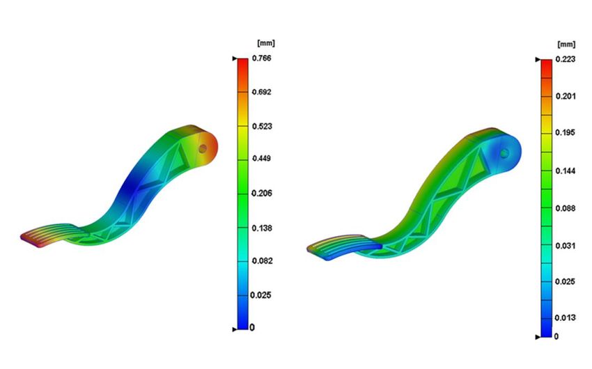
Polymers 2022, 14, 2578 13 of 23

 Figure 4. Type of meshing figure.

 According to the three pressure-keeping project results in Table 3, multi-holding ra-
 tio—project II is 90%–75%–60%; the volume shrinkage rate is 12.8%; and the maximum
 warping volume is 3.36 mm, 0.2 mm higher than the original shape; however, the maxi-
 mum locking force is increased by 7.35 Mpa, so maintaining pressure will also increase
 the station loss. The results show that maximum warping occurs at the connection head
 and pedal; the original maximum warping is 0.73; maximum warping is about 0.27 after
 improvement; and the maximum improvement of total warping displacement is 0.46 mm.
 We can see that warping of the connection head part and the front of the pedal signifi-
 cantly improved, and the red area is shifted to an unimportant position, which is of great
 help to the stability and reliability of the part, as shown in Figure 5.

 Table 3. Injection-molding parameter selection table.

 Set Multiple Pressure-Protection Multi-Holding Ra- Multi-Holding Ratio— Multi-Holding Ra-
 Time (s)
 Methods with Different Pressures tio—Project I (%) Project II (%) tio—Project III (%)
 0~4.15 100 90 60
 Time (s) 4.15~5.53 90 75 50
 5.53~6.92 80 60 40
 Volume shrinkage rate Unit of (%) 12.9 12.8 13.1
 Maximum warping volume Unit (mm) 0.78 0.58 0.36
 Average warp volume Unit (mm) 1.86 1.88 2.02
 Maximum mode-locking force Unit (Mpa) 23.86 21.05 13.7

 Figure 5. Comparison of the optimized conformal waterway and the traditional waterway.

Polymers 2022, 14, 2578 14 of 23

 4. Methods
 4.1. Sequence-Approximation Optimization (SAO)
 In general, a multi-objective design optimization is formulated as follows:
 ( 1( ), 2( ), … , ( )) − } (1)
 ∈ where fi (x) is the ith objective function to be minimized and K represents the
 number of objective functions. x = (x1, x2, …, xn). The design variables with n dimensions
 and X feasible regions are represented by T.
 The process parameters in the PIM play a major role in changing the injection cycle
 time and warping. The injection-molding variable factors designed in this paper are: melt
 temperature (Tmelt), filling time (fi), pressure-holding pressure (P), and cooling time (tc).
 The lower and upper limits of the injection-molding parameter factor are shown in Table
 3.
 The first objective function f1 (x) is defined as period time, usually in the explicit form
 of the injection-molding parameter factor, along with cycle time and warping as functions
 to obey, as shown in Equation (2):
 1( ) = + + − (2)
 The change in the warping value is defined as the second objective function, f2 (x).
 The results obtained through numerical simulation in Figure 5 can obviously find the
 change in the warping value of various parts, with the maximum warping value reached
 along with the direction of the right arrow.
 In this paper, by defining two different objective functions as period time and warp-
 ing values, the purpose is to identify the Pareto boundary point by analyzing the above
 two objective functions. Because the object PIM simulation studied in this paper is very
 dense, the identified Pareto boundary points can be considered effective. The general pro-
 cedure of the summarized Sao method for identifying Pareto boundaries is shown in Flow
 Figure 6. The steps are described in the following text:

 Figure 6. Warpage comparison.

 (Part 1) First, the initial value of the sampling point is determined, and the initial sampling
 point is determined by using the Latin hypercube design (LHD) method.

Polymers 2022, 14, 2578 15 of 23

 (Part 2) A simulated numerical analysis of the sampling points is performed, and then
 they are substituted into the target function for the corresponding numerical calculation.
 (Part 3) Because the objective function can be analyzed and calculated through an approx-
 imate RBF network, here, the approximated objective function is marked as ~fi (x) (i = 1, 2,
 …. , K).
 (Part 4) A response surface is found by using the weighted lp norm method, and the Pa-
 reto boundary point is obtained by using the response-surface analysis. The formula is as
 follows:

 1/ 
 [∑ ( ( )) ] − (3)
 =1

 p is the parameter, i (i = 1, 2, K), and indicates the weight of the ith objective function,
 and the weight value is set to 4 via calculation. A set of Pareto-optimal solutions is ob-
 tained by calculating the weights assigned to each design factor. For a Pareto-optimal so-
 lution obtained via substitution Equation (3), the calculation result can be a new sampling
 point to update the response surface, but the algorithm can only achieve local accuracy.
 (Part 5) We use the density function introduced later in this paper to find the area where
 the sampling point is not covered. This minimizes the function by constructing the density
 function first. The optimal solution obtained from the density function is then rearranged
 to serve as a new sampling point value. We repeat the procedure described above to ter-
 minate this procedure with the final criterion. The purpose of introducing this step is to
 distribute the sampling points as evenly as possible, thus laying the foundation for the
 global approximation.
 (Part 6) If the calculation results meet the terminal criteria, the Sao algorithm will not con-
 tinue to run. Instead, we return from this step to step 2.
 The determination of the terminal criterion is as follows: the average error between
 the response-surface value of the Pareto boundary point calculated in part 4 and the nu-
 merical simulation of part 2. In order to ensure the accuracy of the average error, the Sao
 program is set within 5%.
 Figure 6 shows the SAO process for multi-objective optimization issues. In this paper,
 the entire SAO process uses the RBF network, and this paper uses the optimal error be-
 tween the response surface and the numerical simulation as the final criterion of the SAO
 algorithm. First, the initial sampling point is generated using the Latin Hypercube Design
 (LHD). Assuming that the number of sampling points is m, the optimal solution of the
 response surface is obtained by constructing the response surface from the m sampling
 point by using the radial-basis-function network. The error of the target function at the
 optimal solution is investigated. If the error is small, the SAO algorithm is terminated.
 Otherwise, the optimal solution of the response surface acts directly as a new sampling
 point, and the algorithm moves on to the next stage of looking for unexplored areas. At
 this stage, the number of sampling points is updated to m-m1. The goal of this phase is to
 find globally approximate unexplored areas. At this stage, the density function is con-
 structed by a network of radial basis functions. The optimal solution of the density func-
 tion is the new sampling point, and the sample points are updated as shown in Figure 7,
 which introduces parameter counts. This parameter controls the number of sample points
 that the density function can obtain. Therefore, in the proposed algorithm, the number of
 sampling points for density functions varies according to the number of design variables.
 If the parameter count is less than int (n/2), the parameter is increased to count = count1.
 The final criteria for this phase are given by int (n/2), where represents rounding. If the
 endpoint criteria for this phase are met, we will perform a numerical simulation at the
 new sampling point.

Polymers 2022, 14, 2578 16 of 23

 Figure 7. Flow of sequential approximate optimization for multi-objection.

 4.2. RBF Function Network
 The RBF network is a three-layer feed-forward network. The output of the network
 ŷ(x) corresponds to the response surface, where m denotes the number of sampling points,
 hj(x) is the jth basis function, and wj denotes the weight of the jth basis function. The fol-
 lowing Gaussian kernel is generally used as the basis function:
 ( − ) ( − )
 ℎ ( ) = exp⁡(− ) (4)
 2 
 In Equation (4), xj represents the jth sampling point, and rj is the width of the jth
 basis function. The response yj is calculated at the sampling point xj. The learning of RBF
 network is usually accomplished by solving
 
 =∑ ( − ( ))2 + ∑ 2 − (5)
 =1 =1

 The introduction of the second term in the formula is mainly because of the regular-
 ization requirement of Equation (5). Additionally, the value of j (5) in the equation is usu-
 ally as small as possible (for example, j = 1.0102). It infers that the learning ability of the
 RBF network is calculated to determine the weight vector w and the weight value. The
 results of the formula are as follows:
 
 = (6)
 √ 
 where dmax represents the maximum distance between sampling points; n represents the
 number of design variables; and m represents the number of sampling points. Equation

Polymers 2022, 14, 2578 17 of 23

 (6) applies to all base functions. Therefore, r1 = r2 = rm = r. Assume that the proportions of
 all design variables are equal. This scaling technique is called adaptive scaling technology,
 and we consider the K-level full-factor design, where the regular interval is ∆d in this case,
 and the dmax data are determined by:
 = √ ( − 1)Δ (7)
 In the case of n design variables, the number of sampling points m is simply calcu-
 lated as follows:
 = (8)
 We solve (8) about r/∆d, and then, we can finally obtain the following equation:
 −2 1
 = 2 (1 − ) (9)
 Δ 
 It is clear from Equation (10) that the learning of the RBF network is equivalent to the
 matrix inversion (HTH + Λ) − 1. The new sampling points are added through the SAO
 process. The following simple estimate is adopted to determine the width in Equation
 (10):
 , 
 = ⁡⁡⁡⁡⁡⁡ = 1,2, … , , (10)
 √ √ − 1
 Where m is the number of sampling points, n is the number of injection-molding pa-
 rameter factors, and dj is the distance between the jth sampling point and the one furthest
 from it.
 The literature shows that Equation (10) can be successfully applied to the least-
 square-support rectangle machine.
 In Sao’s method process, it is necessary to find a method to find the area where the
 sampling point is uncovered. In order to find the unexplored area using the RBF network,
 the function prediction can be implemented via Kriging’s method, so as to explore the
 area where the sampling point is uncovered using the density function. On how to con-
 struct an appropriate density function and effectively obtain the local optimal solution to
 the region of the sampling point:

 5. Results
 In SAO, it is important to identify unexplored areas that are globally approximated.
 The Kriging method can achieve this through the Expected Improvement (EI) function. In
 order to use the RBF network to find unexplored areas, we developed a function called
 density function. The process of building density functions is summarized below:
 (D-step 1) The following vector yD is prepared at the sampling points.
 (D-step 2) The weight vector wD of the density function
 = (1,1, … ,1) ×1 (11)

 D(x) is calculated as follows:
 = ( + Λ)−1 (12)

 (D-step 3) The density function D(x) is minimized.
 
 ( ) = ∑ 
 ( ) − (13)
 =1

 (D-Step 4) Figure 8 is an experimentally obtained one-dimensional Pareto-optimal solu-
 tion map, or a Pareto boundary point map. It can be seen that the RBF network is basically
 the interpolation between the sampling points, and the black points indicate the sampling
 points. The local minimum is obtained in the region not involved by the sampling point,
 so the P1 and P2 two points in Figure 8 are the maximum and minimum of the injection-

Polymers 2022, 14, 2578 18 of 23

 molding parameter variables of the density function. As shown in Figure 8, a count calcu-
 lation is added, and int () is rounded. If the count is less than int (n/2), the number will
 rise as count = + 1. This parameter limits the range of the number of new sampling points
 obtained via the density function. The density of the function is constantly updated and
 optimized to ensure global approximation as well as homogenization of the sampling
 point.

 Figure 8. Illustrative example of density function in one dimension.

 In this experiment, 15 initial sampling points were extracted using the LHD sampling
 method, and then the injection parameter value of the sampling points was replaced into
 the RBF network for training. We identified the Pareto boundary between the injection
 time and warping shown in the Figure 6 and the Sao flow chart shown in Figure 8. The
 blue rectangular point represents the Pareto boundary point of the traditional cooling
 channel, and the red star point represents the Pareto boundary point of the optimized
 conformal cooling channel.
 From the data points of the experimental results in Figure 8: the value of the confor-
 mal cooling channel over the boundary point of the conventional cooling waterway in-
 creases by 18.4%, and the warping is worth 44.8%. This shows that the conformal cooling
 channel greatly improves the position of the Pareto-optimal solution point compared to
 the traditional cooling channel. In order to more intuitively analyze the experimental data,
 we chose three times—P1, P2 and P3—whose warping time and cycle time are roughly
 the same, and the data points with obvious characteristics. Their numerical data are com-
 pared in Table 4.

 Table 4. Range of research factors.

 Tmelt (°C) fi (s) P (Mpa) tc (s) Range
 260 1.8 10 5 ≧
 280 2.2 14 22 ≦

 From the resulting curve, the higher the temperature of the molten plastic, the greater
 the pressure and time, and it is preferable to reduce warpage. For the simulation analysis
 of the modal flow of the pedal, since the numerical simulations were very dense, in the