TreeSp2Vec: a method for developing tree species embeddings using deep neural networks
←
→
Page content transcription
If your browser does not render page correctly, please read the page content below
TreeSp2Vec: a method for developing tree species embeddings using deep neural networks Miguel A. González-Rodríguez ( miguel.an.gon.ro@gmail.com ) Guangzhou Institute of Geography, Guangdong Academy of Sciences https://orcid.org/0000-0002- 0072-3124 Ulises Diéguez-Aranda Universidade de Santiago de Compostela https://orcid.org/0000-0002-4640-6714 Zhou Ping Guangzhou Institute of Geography, Guangdong Academy of Sciences https://orcid.org/0000-0001- 7983-8495 Research Article Keywords: species classi cation, national forest inventory, representation learning, multi–layer perceptron, arti cial intelligence Posted Date: June 1st, 2022 DOI: https://doi.org/10.21203/rs.3.rs-957638/v4 License: This work is licensed under a Creative Commons Attribution 4.0 International License. Read Full License
1          TreeSp2Vec: a method for developing tree species embeddings
 2                         using deep neural networks
 3                       González-Rodrı́guez, M.A.a,∗, Diéguez-Aranda, U.b , Zhou, P.a
            a
 4           Guangzhou Institute of Geography, Guangdong Academy of Sciences, Guangzhou 510070, China
     b
 5       Unidade de Xestión Ambiental e Forestal Sostible, Departamento de Enxeñarı́a Agroforestal, Universidade
 6                                  de Santiago de Compostela, 27002 Lugo, Spain

 7   Abstract

 8         1. In recent years, Representation Learning (RL), a subdiscipline of artificial intelligence,
 9              has proved a valuable resource in many research fields for mapping abstract categories
10              into numeric scales as a means to boost varied quantitative modeling tasks. Despite
11              the up-and-coming advantages that RL could imply for managing categorical data in
12              ecological modeling, applications in ecology are still lacking. In this study, we proposed
13              a new method for applying RL to forest ecology, labeled TreeSp2Vec, for developing
14              tree species numeric representations (embeddings).
15         2. Our approach entailed a supervised species classification of individual trees using as
16              input a set of phytocentric (morphometrics and composition) and geocentric (climate,
17              soil, and physiography) variables derived from National Forest Inventory data and
18              environmental cartography. Species classification was carried out using deep neural
19              networks with several fully connected layers, an intermediate embedding layer of up
20              to 32 dimensions, and an output layer with softmax activations.
21         3. Among the tested neural network architectures, a multi-layer perceptron with two hid-
22              den layers of 1024 units and an embedding layer of 16 units provided the best apparent
23              and test classification performances (Matthew’s Correlation Coefficient = 0.89). Ad-
24              ditionally, the developed latent representations (W), or embeddings, were evaluated
25              intrinsically by estimating their correlations with supplementary species descriptors
26              that were not included in the training dataset. The evaluation analysis revealed some
27              significant associations that proved the generality of the embedding model. For in-
                                                            1
28           stance, some latent dimensions (e.g., W6 and W16 ) helped differentiate species general
29           features, such as conifers vs. broad-leaved species, while other dimensions (e.g., W2
30           and W5 ) were related to forest ecosystem characteristics such as competition intensity
31           (relative spacing index) and biodiversity (Simpson index).
32      4. We concluded that the developed embeddings provided accurate and generalizable
33           numeric representations of the considered tree species, which can be used as a ground
34           for further cutting-edge forest ecology modeling approaches. Moreover, our approach
35           is easily extendable to other ecological research areas, opening a new range of artificial
36           intelligence applications in ecology.

37   Keywords: species classification, national forest inventory, representation learning,
38   multi–layer perceptron, artificial intelligence

39   1. Introduction

40         Over the last decade, deep neural network models have revolutionized numerous scientific
41   areas due to their unprecedented predictive performance (Sejnowski, 2018). Recent innova-
42   tions in network architectures have paved the path for new and fruitful scientific disciplines
43   (e.g., Computer Vision), frequently included in the broader scope of artificial intelligence
44   (AI). Applications of AI in ecology have been steadily appearing in recent years (Christin
45   et al., 2019), in most cases centered around the field of ecosystem monitoring (Wäldchen and
46   Mäder, 2018). The ecological AI models developed so far use to rely on the most popular
47   disciplines, such as Computer Vision and Audio Recognition, with applications for various
48   tasks such as species identification from images(Wäldchen and Mäder, 2018; Willi et al.,
49   2019) and sounds (Salamon et al., 2017; Kiskin et al., 2020) and remote sensing-based infer-
50   ence of ecosystem properties (Kittlein et al., 2022). However, despite the proliferation of AI
51   applications in ecology, the explored uses of deep neural networks are still scarce compared

       ∗
        Corresponding author
        Email addresses: miguelangel.gonzalez.rodriguez@rai.usc.es (González-Rodrı́guez, M.A. ),
     ulises.dieguez@usc.es (Diéguez-Aranda, U.)
     Preprint                                                                              June 1, 2022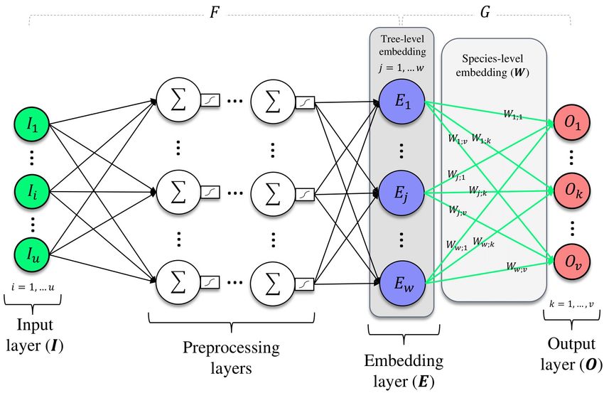
52   to the range of AI disciplines that remain uncharted. In this regard, one of the most notable
53   milestones in the field of AI is the emergence of Representation Learning (RL, Goodfellow
54   et al., 2013; Huang et al., 2014), a relatively unexplored discipline for the ecology research
55   community with potentially promising applications.
56      The primary focus of the RL discipline is the mapping of qualitative objects into numeric
57   scales using deep neural networks. RL models usually take as input a simple numeric
58   encoding of features (e.g., binary variables) that describe the abstract object and transform
59   it into a continuous representation. The resulting quantitative dimensions from this mapping
60   procedure are commonly referred to as “embeddings,” and the vector space defined by them
61   is called “latent” space (Yu et al., 2013). As the latent space typically has lower dimension
62   than the inputs, RL is frequently labeled as a dimensionality reduction technique. However,
63   from a practical modeling perspective, the most relevant implication of RL is the possibility
64   of transforming or encoding categorical variables into ensembles of continuous variables.
65   Thus, abstract and hard to quantify differences between objects (i.e., “semantic” distances)
66   can be easily expressed as algebraic distances in the latent space.
67      RL was initially developed within the field of Natural Language Processing with the
68   purpose of transforming words into numbers for boosting text manipulation quantitative
69   approaches. In this regard, the first and most prominent application of RL was the embed-
70   ding of English words into a 100D latent space with the Word2Vec methodology (Mikolov
71   et al., 2013), which became the backbone of subsequent Natural Language Processing re-
72   search. Since then, a diverse range of applications of RL have been developed in recent
73   years, such as sentence embedding (Tang et al., 2013), biomedical notes embedding (Wang
74   et al., 2018), semantic-based image embedding (Irtaza et al., 2014) and embedding of states
75   in dynamic systems (Lesort et al., 2018; Gelada et al., 2019). Moreover, generative artificial
76   intelligence approaches, such as autoencoders (Goodfellow et al., 2016), also use RL to build
77   the latent space from which the inputs for the generative process are drawn.
78      Despite the recent successful uses of RL in several disciplines, applications in ecology
79   and environmental sciences are still lacking. The up-and-coming contributions of applying
80   RL in ecology are varied and have to do with the ability of embedding models to transform
                                                   3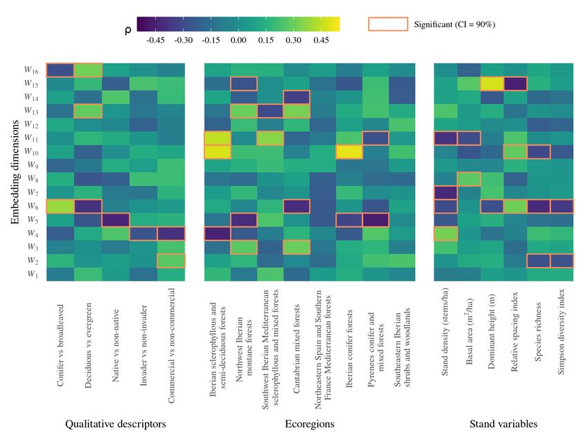
81   usual ecological categories, such as species, populations, and communities, into quantitative
 82   variables. We envisage two main groups of potential ecological applications derived from this
 83   transformation. On the one hand, RL can help to clear frequent information bottlenecks in
 84   ecological research derived from the immiscibility of categorical and numeric data Lindegarth
 85   and Gamfeldt, 2005. On the other hand, the ability of RL to provide reusable representa-
 86   tions Goodfellow et al., 2016 could open a new range of high generality ecological models,
 87   accurately describing the behavior of a variety of species and community types resting on
 88   similar inputs. Regarding the first group of applications, RL could provide crucial upgrades
 89   both for the study of dissimilarity between species, populations, and communities Hao et al.,
 90   2019b as well as for the estimation of biodiversity. For instance, by projecting two different
 91   community types into a latent space, their ecological differences might be estimated simply
 92   as the algebraic distance in this space, thus turning the dissimilarity analysis into a contin-
 93   uous task. On another note, projecting individuals belonging to a community into a latent
 94   space can drastically improve pre-existing biodiversity estimation approaches Ricotta et al.,
 95   2021 for fusing categorical information (e.g., taxonomy and sociological classes) and quanti-
 96   tative variables (e.g., individual morphology and environmental conditions). Concerning the
 97   second group of applications, perhaps the most attractive use case is to streamline ecologi-
 98   cal multi-species modeling based on RL. The representation of different species in a latent
 99   space effectively converts the “species” categorical variable into continuous, thus enabling its
100   addition to other usual numeric predictors for ecosystem dynamics modeling. Considering
101   the current research interest in individual-based ecological models (DeAngelis and Grimm,
102   2014; Cornell et al., 2019), we believe that RL can provide a substantial breakthrough for
103   mixing taxonomic and morphometric information in highly diverse communities.
104      In the current study, we present the very first method for applying RL in forest ecology:
105   an embedding model of tree species, labeled “TreeSp2Vec”, based on deep neural networks.
106   As a case study, we applied our modeling approach to the 40 most relevant forest species
107   in Spain using national forest inventory data and available environmental cartography. To
108   further back the usefulness of our method, we also provide a practical example of multi-
109   species ecological modeling using species embeddings as Supplemental Material.
                                                     4
110 2. Methods
111 2.1. Data sources and preprocessing
112 We used tree-level data of the 40 most frequent species in the Third Spanish National
113 Forest Inventory, accounting to a total of 50K inventory plots and approximately 850K trees.
114 The dataset encompassed a relatively wide range of forest types, including native secondary
115 forests, afforestations with native species, and commercial plantations of exotic species,
116 existing in different Mediterranean and Eurosiberian ecoregions within the country. For
117 details about the characteristics and methodology of the Spanish national forest inventory
118 see the explanation by Alberdi et al. (2010).
119 From this dataset, we computed 44 “phytocentric” descriptors related to two major axes:
120 individual and community morphometrics and neighborhood specific composition. Thus, the
121 set of descriptors included i) the diameter at breast height (cm; breast height = 1.3m) and
122 total height (m) of every tree, ii) the arithmetic means of diameters and heights of all the
123 trees in each plot, and iii) the count of the rest of trees in each plot for every considered
124 species. The latter corresponded to 40 variables resulting from the sum of one-hot encoded
125 vectors (binary variables) representing the presence or absence of other species in the vicinity
126 of each tree. These one-hot vectors were expanded to per-hectare values considering the
127 factors defined by the Spanish National Forest Inventory.
128 Additionally, to enable the representation of habitat characteristics, we derived 26 quan-
129 titative “geocentric” descriptors from available cartography. Among these, there were i) 14
130 physical and chemical soil attributes from the 500 m of spatial resolution maps developed
131 by the European Soil Data Centre (Ballabio et al., 2016, 2019), ii) seven physiography vari-
132 ables derived from a Digital Elevation Model with 200 m of spatial resolution of the National
133 Geographical Institute of Spain (MDT200 CC-BY 4.0 ign.es), and iii) five climate
134 variables from the Wordlclim 2.1 dataset (Fick and Hijmans, 2017) with 1 km of spatial
135 resolution.
5136 2.2. Embedding approach and model training
137 The conventional approach for learning numeric representations in AI is to design an
138 auxiliary supervised task for driving the model optimization process (Yang et al., 2015).
139 Under this setup, the latent representation or embedding is defined by a layer of interme-
140 diate operations necessary for transforming the inputs into the final supervised target. As
141 parameter calibration aims to minimize the error of the auxiliary task, the intermediate rep-
142 resentations are “learned” to efficiently compress the input information relevant to this task.
143 Consequently, choosing the right auxiliary task is crucial for ensuring the “meaningfulness”
144 of the learned representations regarding the represented objects’ abstract characteristics.
145 Considering our purpose to learn numeric representations of tree species, we chose species
146 identification as the auxiliary supervised task. We made this choice based on the premise that
147 developing distinct intermediate representations for every species is essential for accurate
148 differentiation. In other words, to differentiate between various species, the model needs
149 to summarize the specific ecological features encapsulated in the inputs (morphometrics,
150 community composition, and habitat) into a simpler vector space where different species
151 are easier to distinguish. Thus, this simpler vector space (i.e., latent space) is considered
152 to retain nearly the same level of ecological coherency as the inputs, but in a more efficient
153 and interpretable way.
154 For implementing this encoding strategy, in the current study we performed a multi-
155 label classification to identify the species of every tree in the dataset as a function of the
156 previously computed ecological descriptors. Being u the number of input descriptors and v
157 the number of species considered (i.e., the input and output dimension, respectively), and
158 w the dimension of the latent space, the embedding procedure consisted of an “encoder”
159 map F : Ru → Rw , that transforms an input sample into an embedded representation, and
160 a classifier G : Rw → [0, 1]v , that translates the representation into a boolean target. Two
161 types of embedding are derived from this approach. On the one hand, the output of the
162 encoder function F (hereafter, E) is a sample-specific or tree-level embedding with shape
163 n × w, being n the number of samples in the dataset. On the other hand, the set of weight
164 parameters in G with shape v × w (hereafter, W) represents a class-specific or species-level
6165 embedding.
Figure 1: Diagram of the embedding approach using a deep neural network.
166 In the present study, we implemented both transformations, F and G, using deep neural
167 networks (Figure 1). The F map comprised a series of fully connected layers, including the
168 embedding layer (Rw ) as well as preprocessing layers with hyperbolic tangent activations
169 for adding non-linearities. Concerning G, the embedding layer was fully connected to a
170 v-dimensional output layer with softmax activation. We used Tensorflow and the Keras API
171 (Chollet et al., 2015) for Python 3 and GPU acceleration for optimizing different architec-
172 tural variants with one to three preprocessing layers of 64-1024 units and an embedding layer
173 with four to 32 units (scaling in powers of two). The different model variants were fitted
174 using an Adam optimizer for minimizing the categorical cross-entropy loss over a maximum
175 of 5000 epochs. Finally, the trained models were evaluated using a test subset of 20% of the
176 initial dataset basing on the Matthew’s Correlation Coefficient (MCC) implemented in the
177 scikit-learn API (Pedregosa et al., 2011). We chose the MCC as the primary goodness-of-fit
178 indicator over other metrics (e.g., accuracy and precision) because it is more reliable, espe-
7179 cially when working with imbalanced datasets (Chicco and Jurman, 2020). The model with
180 the best validation performance was selected for the subsequent latent space evaluation.
181 As a base for model performance comparison, we also fitted Random Forest classifiers for
182 accomplishing the auxiliary task. Specifically, we fitted two different Random Forest models:
183 i) a “full” model (RL) for predicting the species of every tree using the 70 input descriptors
184 (i.e., emulating both the F and G maps), and ii) a simplified model (RLL ) for performing
185 the classification task taking the latent representations (E) as input (i.e., the same role
186 as G), inspired in the methodology proposed by Salakhutdinov and Hinton (2007). Both
187 Random Forest models were fitted using the scikit-learn API and the Bayesian optimization
188 (bayes opt Python package by Nogueira, 2014) for hyperparameter calibration, coupled with
189 Monte Carlo cross-validation.
190 2.3. Embedding evaluation
191 After selecting the best neural network architecture for species identification, we evalu-
192 ated its latent space’s generality and ecological interpretability. Our approach for this was
193 to test the embeddings’ ability to infer unseen ecological species characteristics. To that
194 end, we analyzed the association between the developed species-level embeddings (W) and
195 supplementary species attributes that were not explicitly included as inputs. Specifically, we
196 estimated point-biserial and Spearman correlations between W and three different groups
197 of variables (hereafter, “test descriptors”):
198 • a set of qualitative descriptors encoded as binary variables representing whether a
199 species is a conifer (conifer = 1, broad-leaved = 0), deciduous (deciduous = 1, evergreen
200 = 0), native (native = 1, non-native = 0), invader (invader = 1, non-invader = 0),
201 or of “commercial interest” (according to recent timber production statistics in Spain;
202 MAGRAMA, 2018);
203 • the relative frequencies of occurrence of each species in the eight ecoregions of Spain,
204 according to the TEOW regionalization (Olson et al., 2001); and
8205 • the by-species mean values of a set of forest stand variables calculated for each inven-
206 tory plot (e.g., basal area, relative spacing, and species richness).
207 In addition, we also evaluated the embeddings subjectively through visualization. To
208 further evaluate and illustrate the usability of the embeddings, an example method for
209 developing multi-species predictive models is presented in Supplemental Material.
210 3. Results
211 3.1. Classification performance
212 The trained neural network models achieved high classification performance, being the
213 minimum test MCC score above 0.80. The more robust architecture in terms of classification
214 performance (apparent MCC = 0.89 and test MCC = 0.87) had two hidden preprocessing
215 layers of 1024 units and 16 embeddings (1024:1024:16). Models including a high number of
216 parameters, such as the architectures with three preprocessing layers or 32 embedding units,
217 yielded very similar yet slightly lower accuracy (see Table 1). Consequently, the model with
218 two hidden layers of 1024 units and 16 embeddings (1.14 × 10⁶ parameters), hereafter la-
219 beled “TreeSp2Vec”, was selected as the best alternative for species representation learning.
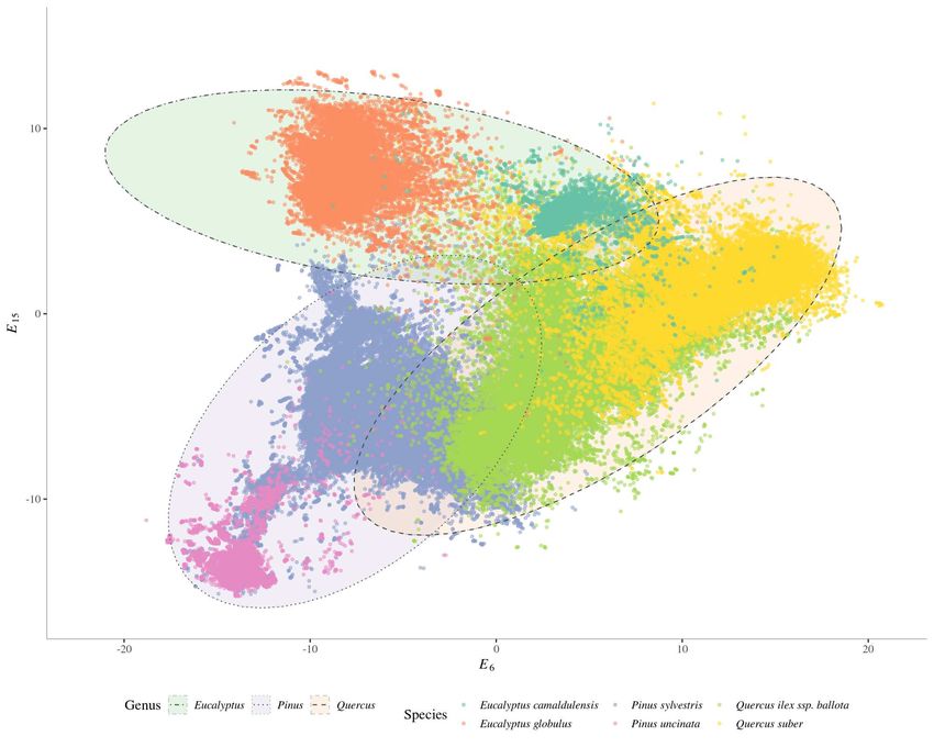
220 Some variations in performance across the set of species for this model were noticed (see
221 the confusion matrix in Figure 2), being the minimum MCC = 0.66 for Populus tremula L.
222 and the maximum MCC = 0.98 for Populus x canadensis Moench. However, no consistent
223 relationship was found between classification performance and species proportions in the
224 dataset, since some very infrequent species, such as Abies pinsapo Boiss. or Chamaecyparis
225 lawsoniana (A. Murray bis) Parl., were accurately classified (MCC = 0.96 and 0.94, respec-
226 tively), while some relatively frequent species, such as Quercus faginea Lam., showed poorer
227 performance (MCC = 0.78). The apparent MCC for every species is shown in Appendix A
228 (Table A.1). The Random Forest model (RF) calibrated for the auxiliary classification task
229 using the 70 input descriptors had 74 trees, a maximum depth of 13, and twelve variables
230 per split. Its performance was notably worse than all the tested neural network architec-
231 tures, yielding a mean MCC = 0.726, with strong variations across species (MCC = 0.956
9232 for Populus x canadensis Moench. but MCC = 0.182 for Salix atrocinerea Brot.). The RFL
233 model, using as input the 16D latent representation produced by the TreeSp2Vec model, had
234 notably better performance (MCC = 0.802) than the standard RF model. This result ac-
235 counts for the feature extraction effectiveness of our representation learning approach since
236 the developed latent space seems to provide an efficient compression of ecological information
237 relevant to species identification.
Figure 2: Confusion matrix (normalized frequencies) of the multi-label classification task using the
TreeSp2Vec model for the 40 species considered.
10Architecture n◦ par. MCC MCCtest
1024:1024:16 1.14×10⁶ 0.892 0.871
1024:1024:32 1.16×10⁶ 0.889 0.870
1024:1024:8 1.13×10⁶ 0.890 0.869
1024:1024:1024:32 2.21×10⁶ 0.887 0.868
1024:1024:1024:16 2.19×10⁶ 0.885 0.866
512:512:32 3.17×10⁵ 0.887 0.866
512:512:512:32 5.79×10⁵ 0.885 0.865
1024:32 1.07×10⁵ 0.881 0.864
512:512:512:16 5.71×10⁵ 0.883 0.863
512:512:16 3.08×10⁵ 0.883 0.863
RF - 0.726 0.702
RFL - 0.803 0.798
Table 1: Classification performance summary of the ten best neural network architectures and Random
Forest models.
11238 3.2. Embedding evaluation
239 The association analysis between the resulting TreeSp2Vec species-level embeddings and
240 the test descriptors (Figure 3) revealed some noticeable relations, which proves the ecological
241 generality of the learned representations. Except for W1 , W9 , and W12 the remaining 13 la-
242 tent dimensions showed significant Spearman and point-biserial correlations, for a confidence
243 level of 90%. Concerning species qualitative attributes, the dimensions W6 and W16 showed
244 intense correlations both with Conif er and Deciduous features, while the dimensions W4
245 and W5 were respectively correlated with N ative and Invader attributes. W2 and W4 were
246 strongly related to the commercial vs. non-commercial dichotomy. Regarding species pres-
247 ence in the TEOW ecoregions, significant correlations with latent dimensions were found for
248 six out of the eight regions considered. Some of the strongest correlations were found for the
249 “Pyrenees conifer and mixed forests” (W5 ), the “Iberian sclerophyllous and semi-deciduous
250 forests” (W4 and W10 ), and the “Iberian conifer forests” (W10 ). The six forest variables
251 were significantly associated with species embeddings. This was especially noticeable for
252 the stand density, which was correlated with four latent dimensions. The two descriptors
253 linked to α-diversity (species richness and the Simpson index) were similarly correlated with
254 dimensions W2 and W6 . W15 was strongly correlated with the dominant height (m) and
255 the relative spacing (also named Hart-Becking index). Besides the one-dimensional anal-
256 ysis, association coherency across latent dimensions was also observed. For instance, W2 ,
257 which seems to be an indicator of “Commercial” species, is also associated with low species
258 richness and Simpson index. W1 1, related to low-density forests, is also an indicator of high
259 presence in open forest formations (“Iberian sclerophyllous and semi-deciduous forests” and
260 “Southwest Iberian Mediterranean sclerophyllous and mixed forests”).
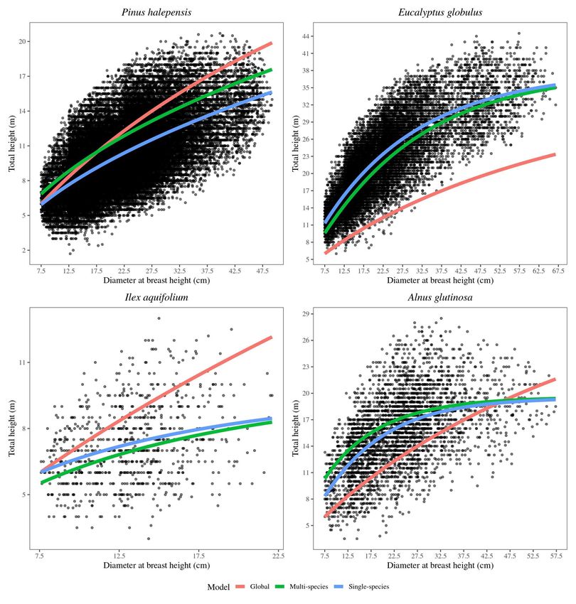
261 The visualization of latent dimensions revealed the existence of patterns (e.g., taxonomic
262 proximity and co-occurrence frequency) that made species easily distinguishable, at least for
263 some dimensions and species. A plot of tree-level embeddings of latent dimensions E6 and
264 E15 is shown in Figure 4.
12Figure 3: Heatmaps of Spearman and point-biserial correlations (ρ) between species-level embeddings and: 1)
qualitative descriptors, 2) presence frequencies in the eight TEOW ecoregions, and 3) mean stand variables.
Significant correlations for a Confidence Interval (CI) of 90% are highlighted.
265 4. Discussion
266 In the field of Representation Learning (RL), the embeddings are considered to efficiently
267 encapsulate the most discriminative portion of information hidden in the data for effectively
268 representing the underlying factors that define abstract relationships between objects (Ben-
269 gio et al., 2013). In the current study, we proposed a novel RL approach to summarize and
270 compress in a continuous latent space the abstract characteristics of tree species present in
271 Spanish forests. As input data, we considered a set of phyto- and geocentric descriptors that
272 represented tree species attributes regarding three major axes: i) tree size (diameters and
13273 heights), ii) specific composition in the vicinity, and iii) habitat characteristics. The high
274 classification performance yielded by the developed neural network models suggests that
275 the proposed architectures were able to extract useful information retained in the inputs
276 and efficiently translate it into a latent space. The latent dimensions resulting from the
277 TreeSp2Vec model seemed to be ecologically meaningful, as they showed significant corre-
278 lations with unseen species features (see Figure 3). The geocentric information provided as
279 input seemed to be effectively encoded by the model, as some latent dimensions proved to
280 be good identifiers of the habitat variability encompassed by the considered ecoregions. In
281 addition, the phytocentric information was effectively compressed by the encoding approach
282 into synthetic representations related to forest variables and specific composition, allowing
283 the latent dimensions to identify species and forest characteristics coherently. For instance,
284 W6 and W16 dimensions seemed to be useful for differentiating between conifers and broad-
285 leaved species, as well as between deciduous and evergreens. W2 proved to be an effective
286 identifier of commercial plantations with low biodiversity (negative correlations with species
287 richness and Simpson index). W8 seemed to be an exclusive identifier of tree species based
288 on forest basal area. The strong relationship between stand density and some dimensions,
289 such as W4 and W11 , provided a valuable criterion for identifying species associated with
290 sparse forests, such as elm oaks and cork oaks, frequent in the Iberian sclerophyllous and
291 semi-deciduous forests. W3 was an exclusive identifier of the Northwest Iberian montane
292 forests and the Cantabrian mixed forests, characterized by deciduous native species (W13 )
293 and non-native plantations of evergreens (W5 and W6 ), which is consistent with the actual
294 characteristics of forests existing in those regions.
295 In the current study, the embedding evaluation procedure was based on correlations
296 with supplementary species descriptors and could be classified as a “concept categorization”
297 intrinsic evaluator, according to the classification proposed by Wang et al. (2019). This
298 method differed notably from the most frequently used approaches in the family of intrin-
299 sic evaluators in RL studies (similarity and analogy evaluators), which compare statistical
300 distances between pairs or groups of objects with subjective similarity rankings previously
301 made by domain experts (Faruqui et al., 2016). In forest ecology, we lack a dataset of human
14302 perceived similarity between species and, consequently, alternative methods for embedding
303 interpretation are necessary. However, even though the evaluation method proposed in the
304 present study proved to be effective for revealing the generality of the encoding approach,
305 the coherency concerning species proximity in the latent space remains unclear. In this
306 regard, visualization proved useful for assessing the ecological coherency in some cases. For
307 instance, in Figure 4 the dimensions E6 and E15 allow to visually distinguish between species
308 belonging to the same genus. In this Figure, species that never occur in the same inventory
309 plot, such as the mountain pine (Pinus uncinata) and eucalypts, are represented far away in
310 the subspace and do not overlap. In contrast, occasional neighbors, such as the Scots pines
311 and cork oaks occurring in forests of central and northern Spain or the elm oaks and the river
312 red gums (Eucalyptus camaldulensis) that can be present in southwestern forests, overlap
313 partially. Regardless of the evaluation approach, the coherency of the latent space could
314 be enhanced by implementing regularization approaches, such as variational architectures,
315 which have demonstrated excellent properties in previous studies for generative-oriented en-
316 coding (Pu et al., 2016; Kingma and Welling, 2014). Derived from this, the development of
317 a variational embedding model for tree species might be a key improvement line in future
318 research.
319 Concerning model performance, the variations in MCC observed across the set of species
320 might have implications regarding the uncertainty of the developed latent representations.
321 It is reasonable to think that latent vectors corresponding to species with low MCC values
322 will have more uncertainty regarding the ecological meaningfulness of their representations.
323 Though there is not an objectively definable threshold for accepting or rejecting the classifi-
324 cation metrics yielded by the TreeSp2Vec model, the fitted random forest classifiers produced
325 much lower scores, which suggests that the species considered in this study were adequately
326 classified overall. Even so, complementary methods for analyzing the potential interactions
327 between performance and ecological coherency might be necessary for clearing this matter
328 in future research.
329 The superior performance of the latent approach (RFL ) versus the standard random
330 forest model (RF) is revelatory of the latent space’s quality. The TreeSp2Vec model effi-
15331 ciently filtered and compressed the input information into 16-dimensional representations
332 that were meaningful enough to boost species identification when coupled with an indepen-
333 dent classifier. This finding offers a promising perspective regarding the reusability of latent
334 representations for other predictive purposes.
335 Considering the adequate model performance and ecological coherency results, we be-
336 lieve that the tree species embeddings developed in the current study might be a valuable
337 resource for other forest ecology research areas. Admittedly, one of the key properties of
338 RL is the ability to transfer learned knowledge from the original auxiliary task to multiple
339 new predictive tasks, thus boosting their performance based on shared statistical strengths.
340 On this basis, the species-level embeddings can be used as input for multi-species predictive
341 modeling tasks by representing the different target species by their corresponding latent
342 vector instead of a categorical variable. In this case, testing the predictive ability of an
343 embedding-based multi-species model in comparison to single-species models can provide
344 a criterion for ecological coherency evaluation from an extrinsic perspective (as shown in
345 Supplemental Material). Apart from multi-species predictive modeling, the use of species-
346 level embeddings could enhance previous methodologies for biological similarity estimation
347 between forest types (Hao et al., 2019a; Ricotta et al., 2021), by providing a supervised
348 framework for integrating non-linear relationships and interactions of varied tree and habi-
349 tat descriptors. In this regard, two major improvement lines could be proposed: i) the
350 development of new metrics for assessing the heterogeneity of the latent space in terms of
351 biodiversity, similarly to traditional indexes (e.g., the Avalanche Index, Ganeshaiah et al.,
352 1997), and, ii) the addition of new species descriptors for representing morphological diver-
353 sity and functional traits (Hao et al., 2019b). Moreover, the inclusion of spatial (e.g., spatial
354 distribution indexes) and temporal (e.g., growth estimations derived from plot remeasure-
355 ments) descriptors could be crucial improvements for developing numeric representations of
356 tree species considering forest structure and dynamics. These developments would provide
357 relevant advantages for future forest ecology research.
358 Although the RL approach presented in the current study is specific to forest ecology,
359 it can be easily extended to other areas. Incorporating individual morphometrics and habi-
16360 tat numeric variables does not require additional area-specific preprocessing, which eases
361 its application in the broader spectrum of ecological sciences. Moreover, the flexibility of
362 deep neural networks for taking inputs of varied dimensionality allows for the implementa-
363 tion of complex quantitative morphometrics (e.g., elliptical Fourier transforms of individual
364 shapes), which are currently popular in many areas of ecology (Caillon et al., 2018). Regard-
365 ing community composition variables, since traditional encoding techniques, such as binary
366 variables (1=presence, 0=absence), are a widespread resource in ecology (?), the extrapola-
367 tion of our RL approach to other areas should be straightforward. Considering the above,
368 we believe that our embedding method for learning numeric representations of tree species
369 opens a new range of artificial intelligence applications in ecology.
370 5. Author contributions
371 Conceptualization, M.A. González-Rodrı́guez, and U. Diéguez-Aranda; software, vali-
372 dation, formal analysis, investigation, data curation, visualization, writing—original draft
373 preparation, M.A. González-Rodrı́guez; methodology, resources, writing—review and edit-
374 ing, M.A. González-Rodrı́guez, U. Diéguez-Aranda and P. Zhou; supervision, project ad-
375 ministration, funding acquisition, U. Diéguez-Aranda and P. Zhou.
376 6. Acknowledgements
377 We thank the Banco de Datos de la Naturaleza (BDN) for the Third National Forest
378 Inventory data provided. We also thank the IGN for the digital elevation model provided,
379 the ESDAC for the soil attributes maps and the Wordlclim 2.1 project for the climate dataset
380 (Fick and Hijmans, 2017).
381 7. Conflict of interest statement
382 The authors declare no conflict of interest.
17383 8. Data availability
384 The input data used in this article is available at the Banco de Datos de la Naturaleza
385 website (miteco.gob.es).
386 References
387 Alberdi, I., Condés, S., Martı́nez, J., Martı́nez, S., de Toda, S., Sánchez, G., Pérez, F., Villanueva, J.,
388 and Vallejo, R. (2010). Spanish national forest inventory. Martı́nez, S.; de Toda, S.; Sánchez, G.;
389 Pérez, F.; Villanueva, J.A.; Vallejo, R.Alberdi, I.; Condés, S.; Martı́nez, J.; Martı́nez, S.; de Toda, S.;
390 Sánchez, G.; Pérez, F.; Villanueva, J.A.; Vallejo, R.¡br/¿Spanish national forest inventory. In National
391 Forest Inventories. Pathways for Common Reporting; Tomppo, E.,¡br/¿Gschwantner, T., Lawrence, M.,
392 McRoberts, R.E., Eds.; Springer: Berlin, Germany, 2010; pp. 527–54.
393 Ballabio, C., Lugato, E., Fernández-Ugalde, O., Orgiazzi, A., Jones, A., Borrelli, P., Montanarella, L., and
394 Panagos, P. (2019). Mapping lucas topsoil chemical properties at european scale using gaussian process
395 regression. Geoderma, 355:113912.
396 Ballabio, C., Panagos, P., and Monatanarella, L. (2016). Mapping topsoil physical properties at european
397 scale using the lucas database. Geoderma, 261:110–123.
398 Bengio, Y., Courville, A., and Vincent, P. (2013). Representation learning: A review and new perspectives.
399 IEEE Transactions on Pattern Analysis and Machine Intelligence, 35(8):1798–1828.
400 Caillon, F., Bonhomme, V., Möllmann, C., and Frelat, R. (2018). A morphometric dive into fish diversity.
401 Ecosphere, 9.
402 Chicco, D. and Jurman, G. (2020). The advantages of the matthews correlation coefficient (mcc) over f1
403 score and accuracy in binary classification evaluation. BMC Genomics, 21:6.
404 Chollet, F. et al. (2015). Keras.
405 Christin, S., Éric Hervet, and Lecomte, N. (2019). Applications for deep learning in ecology. Methods in
406 Ecology and Evolution, 10:1632–1644.
407 Cornell, S. J., Suprunenko, Y. F., Finkelshtein, D., Somervuo, P., and Ovaskainen, O. (2019). A unified
408 framework for analysis of individual-based models in ecology and beyond. Nature Communications,
409 10:4716.
410 DeAngelis, D. L. and Grimm, V. (2014). Individual-based models in ecology after four decades. F1000Prime
411 Reports, 6.
412 Faruqui, M., Tsvetkov, Y., Rastogi, P., and Dyer, C. (2016). Problems with evaluation of word embeddings
413 using word similarity tasks. In Proceedings of the 1st Workshop on Evaluating Vector-Space Representa-
414 tions for NLP, pages 30–35, Berlin, Germany. Association for Computational Linguistics.
18415 Fick, S. E. and Hijmans, R. J. (2017). WorldClim 2: new 1-km spatial resolution climate surfaces for global
416 land areas. International Journal of Climatology.
417 Ganeshaiah, K. N., Chandrashekara, K., and Kumar, A. R. V. (1997). Avalanche index: A new measure of
418 biodiversity based on biological heterogeneity of the communities. Current Science, 73(2):128–133.
419 Gelada, C., Kumar, S., Buckman, J., Nachum, O., and Bellemare, M. G. (2019). DeepMDP: Learning
420 continuous latent space models for representation learning. In Chaudhuri, K. and Salakhutdinov, R.,
421 editors, Proceedings of the 36th International Conference on Machine Learning, volume 97 of Proceedings
422 of Machine Learning Research, pages 2170–2179. PMLR.
423 Goodfellow, I., Bengio, Y., and Courville, A. (2016). Deep Learning. MIT Press. http://www.
424 deeplearningbook.org.
425 Goodfellow, I. J., Erhan, D., Carrier, P. L., Courville, A., Mirza, M., Hamner, B., Cukierski, W., Tang,
426 Y., Thaler, D., Lee, D.-H., Zhou, Y., Ramaiah, C., Feng, F., Li, R., Wang, X., Athanasakis, D., Shawe-
427 Taylor, J., Milakov, M., Park, J., Ionescu, R., Popescu, M., Grozea, C., Bergstra, J., Xie, J., Romaszko,
428 L., Xu, B., Chuang, Z., and Bengio, Y. (2013). Challenges in representation learning: A report on three
429 machine learning contests.
430 Hao, M., Corral-Rivas, J. J., González-Elizondo, M. S., Ganeshaiah, K. N., Nava-Miranda, M. G., Zhang, C.,
431 Zhao, X., and von Gadow, K. (2019a). Assessing biological dissimilarities between five forest communities.
432 Forest Ecosystems, 6.
433 Hao, M., Ganeshaiah, K. N., Zhang, C., Zhao, X., and von Gadow, K. (2019b). Discriminating among forest
434 communities based on taxonomic, phylogenetic and trait distances. Forest Ecology and Management, 440.
435 Huang, P., Huang, Y., Wang, W., and Wang, L. (2014). Deep embedding network for clustering. In 2014
436 22nd International Conference on Pattern Recognition, pages 1532–1537.
437 Irtaza, A., Jaffar, M. A., Aleisa, E., and Choi, T.-S. (2014). Embedding neural networks for semantic
438 association in content based image retrieval. Multimedia Tools and Applications, 72.
439 Kingma, D. P. and Welling, M. (2014). Auto-encoding variational bayes.
440 Kiskin, I., Zilli, D., Li, Y., Sinka, M., Willis, K., and Roberts, S. (2020). Bioacoustic detection with
441 wavelet-conditioned convolutional neural networks. Neural Computing and Applications, 32:915–927.
442 Kittlein, M. J., Mora, M. S., Mapelli, F. J., Austrich, A., and Gaggiotti, O. E. (2022). Deep learning
443 and satellite imagery predict genetic diversity and differentiation. Methods in Ecology and Evolution,
444 13:711–721.
445 Lesort, T., Dı́az-Rodrı́guez, N., Goudou, J.-F., and Filliat, D. (2018). State representation learning for
446 control: An overview. Neural Networks, 108:379–392.
447 Lindegarth, M. and Gamfeldt, L. (2005). Comparing categorical and continuous ecological analyses: Effects
448 of ”wave exposure” on rocky shores. Ecology, 86:1346–1357.
19449 MAGRAMA (2018). Anuario de estadı́stica forestal 2018.
450 Mikolov, T., Sutskever, I., Chen, K., Corrado, G. S., and Dean, J. (2013). Distributed representations of
451 words and phrases and their compositionality. In Burges, C. J. C., Bottou, L., Welling, M., Ghahramani,
452 Z., and Weinberger, K. Q., editors, Advances in Neural Information Processing Systems, volume 26.
453 Curran Associates, Inc.
454 Nogueira, F. (2014). {Bayesian Optimization}: Open source constrained global optimization tool for
455 {Python}.
456 Olson, D. M., Dinerstein, E., Wikramanayake, E. D., Burgess, N. D., Powell, G. V. N., Underwood, E. C.,
457 D’amico, J. A., Itoua, I., Strand, H. E., Morrison, J. C., Loucks, C. J., Allnutt, T. F., Ricketts, T. H.,
458 Kura, Y., Lamoreux, J. F., Wettengel, W. W., Hedao, P., and Kassem, K. R. (2001). Terrestrial Ecoregions
459 of the World: A New Map of Life on Earth: A new global map of terrestrial ecoregions provides an
460 innovative tool for conserving biodiversity. BioScience, 51(11):933–938.
461 Pedregosa, F., Varoquaux, G., Gramfort, A., Michel, V., Thirion, B., Grisel, O., Blondel, M., Prettenhofer,
462 P., Weiss, R., Dubourg, V., Vanderplas, J., Passos, A., Cournapeau, D., Brucher, M., Perrot, M., and
463 Duchesnay, E. (2011). Scikit-learn: Machine learning in Python. Journal of Machine Learning Research,
464 12:2825–2830.
465 Pu, Y., Gan, Z., Henao, R., Yuan, X., Li, C., Stevens, A., and Carin, L. (2016). Variational autoencoder
466 for deep learning of images, labels and captions. In Lee, D., Sugiyama, M., Luxburg, U., Guyon, I., and
467 Garnett, R., editors, Advances in Neural Information Processing Systems, volume 29. Curran Associates,
468 Inc.
469 Richards, F. J. (1959). A flexible growth function for empirical use. Journal of Experimental Botany,
470 10:290–300.
471 Ricotta, C., Szeidl, L., and Pavoine, S. (2021). Towards a unifying framework for diversity and dissimilarity
472 coefficients. Ecological Indicators, 129:107971.
473 Salakhutdinov, R. and Hinton, G. (2007). Learning a nonlinear embedding by preserving class neighbourhood
474 structure. volume 2, pages 412–419. PMLR.
475 Salamon, J., Bello, J. P., Farnsworth, A., and Kelling, S. (2017). Fusing shallow and deep learning for
476 bioacoustic bird species classification. pages 141–145. IEEE.
477 Sejnowski, T. (2018). The Deep Learning Revolution. The MIT Press. MIT Press.
478 Tang, D., Qin, B., Liu, T., and Li, Z. (2013). Learning sentence representation for emotion classification
479 on microblogs. In Zhou, G., Li, J., Zhao, D., and Feng, Y., editors, Natural Language Processing and
480 Chinese Computing, pages 212–223, Berlin, Heidelberg. Springer Berlin Heidelberg.
481 Wang, B., Wang, A., Chen, F., Wang, Y., and Kuo, C.-C. J. (2019). Evaluating word embedding models:
482 methods and experimental results. APSIPA Transactions on Signal and Information Processing, 8:e19.
20483 Wang, Y., Liu, S., Afzal, N., Rastegar-Mojarad, M., Wang, L., Shen, F., Kingsbury, P., and Liu, H. (2018).
484 A comparison of word embeddings for the biomedical natural language processing. Journal of Biomedical
485 Informatics, 87.
486 Willi, M., Pitman, R. T., Cardoso, A. W., Locke, C., Swanson, A., Boyer, A., Veldthuis, M., and Fortson, L.
487 (2019). Identifying animal species in camera trap images using deep learning and citizen science. Methods
488 in Ecology and Evolution, 10:80–91.
489 Wäldchen, J. and Mäder, P. (2018). Machine learning for image based species identification. Methods in
490 Ecology and Evolution, 9:2216–2225.
491 Yang, S., Luo, P., Loy, C. C., Shum, K. W., and Tang, X. (2015). Deep representation learning with target
492 coding. Proceedings of the AAAI Conference on Artificial Intelligence, 29(1).
493 Yu, W., Zeng, G., Luo, P., Zhuang, F., He, Q., and Shi, Z. (2013). Embedding with autoencoder regulariza-
494 tion. In Blockeel, H., Kersting, K., Nijssen, S., and Železný, F., editors, Machine Learning and Knowledge
495 Discovery in Databases, pages 208–223, Berlin, Heidelberg. Springer Berlin Heidelberg.
496 Appendix A. Classification performance by species
21Figure 4: Scatterplot of 6th vs 15th dimensions of tree-level embeddings for Pinus uncinata Ramond ex
A.DC., Pinus sylvestris L., Quercus ilex L. ssp. ballota, Quercus suber L., Eucalyptus globulus Labill., and
Eucalyptus camaldulensis Dehnh. Shaded ellipses correspond to confidence intervals = 99% of by-genus
multivariate normal distributions.
22Species MCC
Chamaecyparis lawsoniana 0.938
Pinus sylvestris 0.903
Pinus uncinata 0.931
Pinus pinea 0.875
Pinus halepensis 0.945
Pinus nigra 0.875
Pinus pinaster 0.918
Pinus radiata 0.943
Abies alba 0.853
Abies pinsapo 0.955
Pseudotsuga menziesii 0.927
Juniperus thurifera 0.829
Quercus robur 0.794
Quercus petraea 0.819
Quercus pyrenaica 0.914
Quercus faginea 0.787
Quercus ilex ssp. ballota 0.878
Quercus suber 0.857
Quercus canariensis 0.755
Quercus rubra 0.879
Populus alba 0.892
Populus tremula 0.658
Alnus glutinosa 0.798
Fraxinus angustifolia 0.785
Populus nigra 0.913
Eucalyptus globulus 0.931
Eucalyptus camaldulensis 0.960
Ilex aquifolium 0.734
Olea europaea 0.814
Fagus sylvatica 0.926
Castanea sativa 0.841
Corylus avellana 0.786
Robinia pseudoacacia 0.750
Quercus pubescens 0.718
Fraxinus excelsior 0.662
Salix alba 0.738
Populus x canadensis 0.975
Betula alba 0.747
Salix atrocinerea 0.677
Betula pendula 0.718
Table A.1: Mathew’s Correlation Coefficient of the classification task performed by the TreeSp2Vec model
for each of the 40 species considered.
23Supplemental Material
TreeSp2Vec: a method for developing tree species em-
beddings using deep neural networks
S-I. Example of embedding-based multi-species modelling
We present a simple illustrative example of how to use species-level embeddings for
developing empirical multi-species models. The task is to develop a multi-species generalized
height-diameter (h-d) equation for predicting the total height of individual trees as a function
of their diameter at breast height.
S-I.1. Example methods
The proposed h-d model for this example is the Chapman-Richards equation (Richards,
1959):
c
h = 1.3 + a 1 − exp(−bd) , (S1)
where h is the tree total height (m), d is the tree diameter at breast height (cm), and a,
b and c are parameters. We fit the Chapman-Richards equation for the 30 most frequent
species in the dataset by developing 1) one global generalized h-d model (i.e., with the same
a, b and c values for all the species) and 2) 30 different single-species models. Then, the
parameters (a, b and c) in each single-species model are expanded using the species-level
embeddings. We do so by predicting a, b and c as a function of the previously developed
16 latent dimensions (W) using a machine learning model. Specifically, we use multi-layer
perceptrons (MLPs) with three hidden layers of 32 units and ReLU activations, calibrated
through Monte Carlo validation. Finally, we apply the expanded a, b and c parameters for
each species for re-predicting the total tree height using a multi-species Chapman-Richards
model: M LPc (W)
h = 1.3 + M LPa (W) 1 − exp − M LPb (W)d , (S2)
where M LPx are the outputs of the multilayer perceptrons trained for predicing a, b and c
as a function of W.
1S-I.2. Example results
As expected, considering the variety of species in the dataset, the global h-d model
performs very poorly (see Table S1), yielding an R2 =0.49, being the unweighted mean over
the set of species R2 =0.05. In comparison, the single-species models perform much better,
although they also show strong variations in R2 between different species (ranging from
R2 =0.32 to 0.73, see Figure S1). The three parameters are succesfully predicted from the
latent dimensions (see Figure S2), which accounts for the existence of meaningful associations
with W. Finally, the re-prediction of tree height using the multi-species Chapman-Richards
model reveals, on average, only in a slight drop in performance with respect to the single-
species models (see Figure S3). This result confirms the usefulness of the approach for using
only one model for all the species while maintaining good performance.
Model R2 2
Rmin 2
Rmean 2
Rmax
Global 0.485 -0.502 0.0566 0.501
Single-species 0.736 0.322 0.504 0.7308
Multi-species 0.662 0.0929 0.455 0.7208
Table S1: Predictive performance of the developed h-d approaches.
2Figure S1: Violin plots representing the distribution of R2 across species of the three h-d modeling ap-
proaches.
Figure S2: Observed vs predicted values of the parameters using the three MLP models.
3Figure S3: h-d scatter plots of four tree species with predicted trends for the three generalized h-d model
approaches.
4You can also read