Learning Signal-Agnostic Manifolds of Neural Fields - arXiv
←
→
Page content transcription
If your browser does not render page correctly, please read the page content below
Learning Signal-Agnostic Manifolds of Neural Fields

                                                   Yilun Du1        Katherine Collins1,2     Joshua B. Tenenbaum1,2,3        Vincent Sitzmann1
                                             yilundu@mit.edu          katiemc@mit.edu                jbt@mit.edu              sitzmann@mit.edu
                                                                         1
                                                                             MIT CSAIL 2 MIT BCS 3 MIT CBMM
                                                                              https://yilundu.github.io/gem/
arXiv:2111.06387v1 [cs.LG] 11 Nov 2021

                                                                                           Abstract
                                                      Deep neural networks have been used widely to learn the latent structure of datasets,
                                                      across modalities such as images, shapes, and audio signals. However, existing
                                                      models are generally modality-dependent, requiring custom architectures and
                                                      objectives to process different classes of signals. We leverage neural fields to
                                                      capture the underlying structure in image, shape, audio and cross-modal audiovisual
                                                      domains in a modality-independent manner. We cast our task as one of learning
                                                      a manifold, where we aim to infer a low-dimensional, locally linear subspace in
                                                      which our data resides. By enforcing coverage of the manifold, local linearity, and
                                                      local isometry, our model — dubbed GEM — learns to capture the underlying
                                                      structure of datasets across modalities. We can then travel along linear regions of
                                                      our manifold to obtain perceptually consistent interpolations between samples, and
                                                      can further use GEM to recover points on our manifold and glean not only diverse
                                                      completions of input images, but cross-modal hallucinations of audio or image
                                                      signals. Finally, we show that by walking across the underlying manifold of GEM,
                                                      we may generate new samples in our signal domains1 .

                                         1        Introduction
                                         Every moment, we receive and perceive high-dimensional signals from the world around us. These
                                         signals are in constant flux; yet remarkably, our perception system is largely invariant to these
                                         changes, allowing us to efficiently infer the presence of coherent objects and entities across time.
                                         One hypothesis for how we achieve this invariance is that we infer the underlying manifold in which
                                         perceptual inputs lie [1], naturally enabling us to link high-dimensional perceptual changes with
                                         local movements along such a manifold. In this paper, we study how we may learn and discover a
                                         low-dimensional manifold in a signal-agnostic manner, over arbitrary perceptual inputs.
                                         Manifolds are characterized by three core properties [2, 3]. First, a manifold should exhibit data
                                         coverage, i.e., all instances and variations of a signal are explained in the underlying low-dimensional
                                         space. Second, a manifold should be locally metric, enabling perceptual manipulation of a signal
                                         by moving around the surrounding low-dimensional space. Finally, the underlying structure of a
                                         manifold should be globally-consistent; e.g. similar signals should be embedded close to one another.
                                         Existing approaches to learning generative models, such as GANs [4], can be viewed as instances of
                                         manifold learning. However, such approaches have two key limitations. First, low-dimensional latent
                                         codes learned by generative models do not satisfy all desired properties for a manifold; while the
                                         underlying latent space of a GAN enables us to perceptually manipulate a signal, GANs suffer from
                                         mode collapse, and the underlying latent space does not cover the entire data distribution. Second,
                                         existing generative architectures are biased towards particular signal modalities, requiring custom
                                         architectures and losses depending on the domain upon which they are applied – thereby preventing
                                         us from discovering a manifold across arbitrary perceptual inputs in a signal-agnostic manner.
                                              1
                                                  Code and additional results are available at https://yilundu.github.io/gem/.

                                         35th Conference on Neural Information Processing Systems (NeurIPS 2021).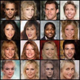
As an example, while existing generative models of images are regularly based on convolutional
neural networks, the same architecture in 1D does not readily afford high-quality modeling of audio
signals. Rather, generative models for different domains require significant architecture adaptations
and tuning. Existing generative models are further constrained by the common assumption that
training data lie on a regular grid, such as grids of pixels for images, or grids of amplitudes for audio
signals. As a result, they require uniformly sampled data, precluding them from adequately modeling
irregularly sampled data, like point clouds. Such a challenge is especially prominent in cross-modal
generative modeling, where a system must jointly learn a generative model over multiple signal
sources (e.g., over images and associated audio snippets). While this task is trivial for humans – we
can readily recall not only an image of an instrument, but also a notion of its timbre and volume –
existing machine learning models struggle to jointly fit such signals without customization.
To obtain signal-agnostic learning of manifolds
over signals, we propose to model distributions
of signals in the function space of neural fields,
which are capable of parameterizing image, au-
dio, shape, and audiovisual signals in a modality-
independent manner. We then utilize hypernet-                 z
works [5], to regress individual neural fields
from an underlying latent space to represent a
                                                         Latent Manifold
signal distribution. To further ensure that our dis-
tribution over signals corresponds to a manifold,
we formulate our learning objective with explicit Figure 1: GEM learns a low-dimensional latent mani-
losses to encourage the three desired properties fold over signals. Given a cross-modal signal, latents in
for a manifold: data coverage, local linearity, GEM are mapped, using a hypernetwork ψ, into neural
and global consistency. The resulting model, networks φ1 and φ2 . φ1 represents a image by mapping
which we dub GEM2 , enables us to capture the each pixel position (x, y) to its associated color c(x, y).
manifold of a variety of signals – ranging from φ2 represents an audio spectrogram by mapping each
audio to images and 3D shapes – with almost no pixel position (u, v) to its intensity w(u, v). This en-
architectural modification, as illustrated in Fig- ables GEM to be applied in a domain agnostic manner
ure 1. We further demonstrate that our approach across separate (multi-modal) signals, by utilizing a sep-
                                                     arate function φ for each mode of a signal.
reliably recovers distributions over cross-modal
signals, such as images with a correlated audio snippet, while also eliciting sample diversity.
We contribute the following: first, we present GEM, which we show can learn manifolds over images,
3D shapes, audio, and cross-modal audiovisual signals in a signal-agnostic manner. Second, we
demonstrate that our model recovers the global structure of each signal domain, permitting easy
interpolation between nearby signals, as well as completion of partial inputs. Finally, we show that
walking along our learned manifold enables us to generate new samples for each modality.

2       Related Work

Manifold Learning. Manifold learning is a large and well-studied topic [2, 3, 6–10] which seeks to
obtain the underlying non-linear, low-dimensional subspace in which naturally high-dimensional input
signals lie. Many early works in manifold learning utilize a nearest neighbor graph to obtain such a
low-dimensional subspace. For instance, Tenenbaum et al. [2] employs the geodesic distance between
nearby points, while Roweis et al. [3] use locally linear subregions around each subspace. Subsequent
work has explored additional objectives [7–10] to obtain underlying non-linear, low-dimensional
subspaces. Recently, [11–13] propose to combine traditional manifold learning algorithms with deep
networks by training autoencoders to explicitly encourage latents to match embeddings obtained from
classical manifold learning methods. Further, [14] propose to utilize a heat kernel diffusion process
to uncover the underlying manifold of data. In this work, we show how we may combine insights
from earlier works in manifold learning with modern deep learning techniques to learn continuous
manifolds of data in high-dimensional signal spaces. Drawing on these two traditions enables our
model to smoothly interpolate between samples, restore partial input signals, and further generate
new data samples in high-dimensional signal space.

    2
        short for GEnerative Manifold learning

                                                    2
Learning Distributions of Neural Fields. Recent work has demonstrated the potential of treating
fully connected networks as continuous, memory-efficient implicit (or coordinate-based) representa-
tions for shape parts [15, 16], objects [17–20], or scenes [21–24]. Sitzmann et al. [25] showed that
these coordinate-based representations may be leveraged for modeling a wide array of signals, such
as audio, video, images, and solutions to partial differential equations. These representations may
be conditioned on auxiliary input via conditioning by concatenation [17, 26], hypernetworks [21],
gradient-based meta-learning [27], or activation modulation [28]. Subsequently, they may be em-
bedded in a generative adversarial [28, 29] or auto-encoder-based framework [21]. However, both
of these approaches require modality-dependent architecture choices. Specifically, modification is
necessary in the encoder of auto-encoding frameworks, or the discriminator in adversarial frameworks.
In contrast, we propose to represent the problem of learning a distribution as one of learning the
underlying manifold in which the signals lie, and show that this enables signal-agnostic modeling.
Concurrent to our work, Dupont et al. [30] propose a signal-agnostic discriminator based on pointwise
convolutions, which enables discrimination of signals that do not lie on regular grids. In contrast, we
do not take an adversarial approach, thereby avoiding the need for a convolution-based discriminator.
We further show that our learned manifold better captures the underlying data manifold and demon-
strate that our approach is able to capture manifolds across cross-modal distributions, which we find
destabilizes training of [30].
Generative Modeling. Our work is also related to existing work in generative modeling. GANs
[4] are a popular framework used to model modalities such as images [31] or audio [32], but often
suffer from training instability and mode collapse. VAEs [33], another class of generative models,
utilize an encoder and decoder to learn a shared latent space for data samples. Recently autoregressive
models have also been used for image [34], audio [35], and multi-modal text and image generation
[36]. In contrast to previous generative approaches, which require custom architectures for encoding
and decoding, our approach is a modality-independent method for generating samples distribution
and presents a new view of generative modeling: one of learning an underlying manifold of data.

3   Parameterizing Spaces of Signals with Neural Fields

An arbitrary signal I in RD1 ×···×Dk can be represented efficiently as a function Φ which maps each
coordinate x ∈ Rk to the value v of the feature coordinate at that dimension.
                                   Φ : Rk → R,      x → Φ(x) = v                                    (1)
Such a formulation enables us to represent any signal, such as an image, shape, or waveform – or
a set of signals, like images with waveforms – as a continuous function Φ. We use a three-layer
multilayer perceptron (MLP) with hidden dimension 512 as our Φ. Only the input dimension of Φ is
varied, depending on the dimensionality of the underlying signal – all other architectural choices are
the same across signal types. We refer to Φ as a neural field.
Parameterizing Spaces over Signals. A set of signals may be parameterized as a subspace F of
functions Φi . To efficiently parameterize functions Φ, we represent each Φ using a low-dimensional
latent space in Rn and map latents to F via a hypernetwork Ψ:
                                  Ψ : Rn → F,       z → Ψ(z) = Φ,                                   (2)

To regress Φ with our hypernetwork, we predict individual weights W L and biases bL for each layer
L in Φ. Across all experiments, our hypernetwork is parameterized as a three-layer MLP (similar to
our Φ), where all weights and biases of the signal representation Φ are predicted in the final layer.
Directly predicting weights W L is a high-dimensional regression problem, so following [37], we
parameterize W via a low-rank decomposition as W L = WsL σ(WhL ), where σ is the sigmoid
function. WsL is shared across all predicted Φ, while WhL = AL ×B L is represented as two low-rank
matrices AL and B L – and is regressed separately for each individual latent z.

4   Learning Structured Manifold of Signals
                                                                             D1 ×···×Dk
Given a training set C = {Ii }N i=1 , of N distinct arbitrary signals Ii ∈ R            , our goal is to
learn – in a signal-agnostic manner – the underlying low-dimensional manifold M ⊂ RD1 ×···×Dk . In

                                                   3
(a) Reconstruction Loss (b) Local Isometry Loss (c) LLE Loss
ReLU
ReLU
Linear
Linear
Linear
...
LeakyReLU
LeakyReLU
Linear
Linear
Linear
Hypernetwork Latent Manifold
Figure 2: GEM learns to embed an arbitrary signal I in a latent manifold via three losses: (a) a reconstruction
loss which encourages neural network φ, decoded from z1 through a hypernetwork, to match training signal I1
at each coordinate x, (b) a local isometry loss to enforce perceptual consistency, which encourages distance
between nearby latents z1 and z2 to be porportional to their distance in signal space I1 , I2 , (c) a LLE loss
which encourages a latent z1 to be represented as a convex combination αi of its neighbors.
particular, a manifold M [2, 3], over signals I, is a locally low-dimensional subspace consisting and
describing all possible variations of I. A manifold has three crucial properties. First, it must embed
all possible instances of I. Second, M should be locally metric around each signal I, enabling us to
effectively navigate and interpolate between nearby signals. Finally, it must be locally perceptually
consistent; nearby points on M should be similar in identity. To learn a manifold M with these
properties, we introduce a loss for each property: LRec , LLLE , and LIso , respectively. LRec ensures that
all signals I are embedded inside M (Section 4.1), LLLE forces the space near each I to be locally
metric (Section 4.2), and LIso encourages the underlying manifold to be perceptually consistent
(Section 4.3). As such, our training loss takes the form:
LTotal = LRec + LLLE + LIso (3)
Please see Fig. 2 for an overview of the proposed manifold learning approach. We utilize equal
weighting across each introduced loss term. We discuss each component of the loss in more detail
below.
4.1 Data Coverage via Auto-Decoding
Given a parameterization of a subspace F (as introduced in Section 3) which represents our manifold
M, we must ensure that Ψ, our hypernetwork, can effectively cover the entire subspace in which our
signal I lies. A common approach to learn subspaces over signals is to employ a GAN [4], whereby
a discriminator trains a hypernetwork Ψ(z) to generate signals that are indistinguishable from real
examples. However, an issue with such an approach is that many I may be missing in the resultant
mapping.
Here, to ensure that our manifold covers all instances, we utilize the auto-decoder framework [17, 21].
We learn a separate latent zi for each training signal Ii and train models utilizing the loss
LRec = kΨ(zi )(x) − Ii (x)k2 (4)
over each possible input coordinate x. By explicitly learning to reconstruct each training point in our
latent space, we enforce that our latent space, and thus our manifold M, covers all training signals I.
4.2 Local Metric Consistency via Linear Decomposition
A manifold M is locally metric around a signal I if there exist local linear directions of variation on
the manifold along which the underlying signals vary in a perceptually coherent way. Inspired by
[3], we enforce this constraint by encouraging our manifold to consist of a set of local convex linear
regions Ri in our learned latent space.
We construct these convex linear regions Ri using autodecoded latents zi (Section 4.1). Each latent
zi defines a convex region, Ri – obtained by combining nearest latent neighbors zi1 , . . . , zij , as
illustrated in Figure 2.
To ensure that our manifold M consists of these convex local regions, during training, we enforce
that each latent zi can be represented in a local convex region, Ri , e.g. that it can be expressed as a
4set of weights wi , such that zi = j wij zij and j wij = 1. Given a zi we may solve for a given
P P
wi by minimizing the objective kzi − j wij zij k2 = wiT Gi wi with respect to wi . In the above
P
expression, Gi is the Gram matrix, and is defined as Gi = kkT , where k is a block matrix, with row
j corresponding to kj = zi − zij . Adding the constraint that all weights add up to one via a Legrange
multiplier, leads to the following optimization objective:
L(wi , λ) = wiT Gi wi + λ(1T wi − 1) (5)
where 1 corresponds to a vector of all ones. Finding the optimal wi in the above expression then
corresponds to the best projection of zi on the linear region Ri it defines. Taking gradients of the
above expression, we find that wi = λ2 G−1 i 1, where λ is set to ensure that elements of wi sum up to
0
P j j
1. The mapped latent zi = j wi zi corresponds to the best projection zi on Ri . To enforce that zi
lies in Ri , we enforce that this projection
LLLE = kΨ(zi0 )(x) − Ii (x)k2 , (6)
also decodes to the training signal Ii , where we differentiate through intermediate matrix operations.
To encourage wi to be positive, we incorporate an additional L1 penalty to negative weights.
4.3 Perceptual Consistency through Local Isometry
Finally, a manifold M should be perceptually consistent. In other words, two signals that are
perceptually similar should also be closer in the underlying manifold, according to a distance metric
on the respective latents, than signals that are perceptually distinct. While in general the MSE distance
between two signals is not informative, when such signals are relatively similar to one another, their
MSE distance does contain useful information.
Therefore, we enforce that the distance between latents zi and zj in our manifold M are locally
isometric to the MSE distance of the corresponding samples Ii and Ij , when relative pairwise
distance of samples is small. On the lowest 25% of pairwise distances, we utilize the following loss:
LIso = kα ∗ k(zi − zj )k − kIi − Ij kk. (7)
Such local isometry may alternatively be enforced by regularizing the underlying Jacobian map.
4.4 Applications
By learning a modality-independent manifold M, GEM permits the following signal-agnostic
downstream applications, each of which we explore in this work.
Interpolation. By directly interpolating between the learned latents zi and zj representing each
signal, we can interpolate in a perceptually consistent manner between neighboring signals in M.
Further, latents for novel signals may be obtained by optimizing LRec on the signal.
Conditional Completion. Given a partial signal Î, we can obtain a point on the manifold M by
optimizing a latent z using LRec + LLLE . Decoding the corresponding latent z then allows us to
complete the missing portions of the image.
Sample Generation. Our manifold M consists of a set of locally linear regions Ri in a underlying
latent space z. As such, new samples in M can be generated by walking along linear regions Ri ,
and sampling points each such region. To sample a random point within Ri , we generate α between
0 and 1, and compute a latent ẑi = αzi + (1 − α) ∗ zij + β ∗ N (0, 1) (corresponding to a random
sample in the neighborhood of zi ) and project it onto the underlying region Ri .
5 Learning Manifolds of Data
We validate the generality of GEM by first showing that our model is capable of fitting diverse signal
modalities. Next, we demonstrate that our approach captures the underlying structure across these
signals; we are not only able to cluster and perceptually interpolate between signals, but inpaint to
complete partial ones. Finally, we show that we can draw samples from the learned manifold of
each signal type, illustrating the power of GEM to be used a signal-agnostic generative model. We
re-iterate that nearly identical architectures and training losses are used across separate modalities.
5StyleGAN2 GEM Ground Truth Modality Model MSE ↓ PSNR ↑
Images
Heat Kernel 0.0365 14.99
VAE 0.0331 15.12
Images
FDN 0.0060 22.59
FDN GEM Ground Truth StyleGAN2 0.0044 24.03
3D Shapes
GEM 0.0025 26.53
VAE 0.0147 18.87
FDN 0.0050 23.68
Audio
StyleGAN2 0.0015 28.52
GEM 0.0011 29.98
StyleGAN2 GEM Ground Truth
FDN 0.0296 16.52
ShapeNet
GEM 0.0153 21.32
Audio-visual
VAE 0.0193 17.23
FDN 0.0663 11.78
Image and Audio
StyleGAN2 0.0063 22.36
GEM 0.0034 24.38
Figure 3: Test-time reconstruction. Comparison of GEM against baselines on the task of fitting test signals
over a diverse set of signal modalities: images, 3D shapes, and audio-visual, respectively. GEM (center)
achieves significantly better reconstruction performance – qualitatively and quantitatively – on test signals than
StyleGAN2 or FDN, indicating better coverage of the data manifold across all modalities. Results are run across
one seed, but we report results across three seeds in the appendix, and find limited overall variance.
Datasets. We evaluate GEM on four signal modalities: image, audio, 3D shape, and cross-modal
image and audio signals, respectively. For the image modality, we investigate performance on the
CelebA-HQ dataset [38] fit on 29000 64 × 64 training celebrity images, and test on 1000 64 × 64
test images. To study GEM behavior on audio signals, we use the NSynth dataset [39], and fit on a
training set of 10000 one-second 16kHz sounds clips of different instruments playing, and test of
5000 one-second 16kHz sound clips. We process sound clips into spectrograms following [32]. For
the 3D shape domain, we work with the ShapeNet dataset from [40]. We train on 35019 training
shapes at 64 × 64 × 64 resolution and test on 8762 shapes at 64 × 64 × 64 resolution. Finally, for
the cross-modal image and audio modality, we utilize the cello image and audio recordings from the
Sub-URMP dataset [41]. We train on 9800 images at 128 × 128 resolution and 0.5 second 16kHz
audio clips, which are also processed into spectrograms following [32] and test on 1080 images and
associated audio clips. We provide additional cross-modal results in the supplement.
Setup and Baselines. We benchmark GEM against existing manifold learning approaches.
Namely, we compare our approach with that of StyleGAN2 [31], VAE [42], and concurrent work
FDN of [30], as well as heat kernel manifold learning [14]. We utilize the authors’ provided codebase
for StyleGAN2, the PytorchVAE library 3 for the VAE, and the original codebase of FDN [30], which
the authors graciously provided. We train all approaches with a latent dimension of 1024, and re-scale
the size of the VAE to ensure parameter counts are similar. We report model architecture details in the
appendix. We need to change the architecture of both the VAE and StyleGAN2 baselines, respectively,
in order to preserve proper output dimensions, depending on signal modality. However, we note
that identical architectures readily can and are used for GEM. For fitting cross-modal audiovisual
signals, all models utilize two separate decoders, with each decoder in GEM identical to each other.
Architectural details are provided in the appendix.
5.1 Covering the Data Manifold
We first address whether our model is capable of covering the underlying data distribution of each
modality, compared against our baselines, and study the impact of our losses on this ability.
Modality Fitting. We quantitatively measure reconstruction performance on test signals in Figure 3
and find the GEM outperforms each of our baselines. In the cross-modal domain in particular, we
find that FDN training destabilizes quickly and struggles to adequately fit examples. We illustrate test
signal reconstructions in Figure 3 and Figure 4. Across each modality, we find that GEM obtains
the sharpest samples. In Figure 3 we find that while StyleGAN2 can reconstruct certain CelebA-HQ
3
https://github.com/AntixK/PyTorch-VAE
6FDN GEM Data FDN GEM Data FDN GEM Data
Modality LLLE LIso MSE ↓ PSNR ↑
No No 0.0028 26.11
Keyboard
Image Yes No 0.0025 26.53
Yes Yes 0.0024 26.69
No No 0.0020 27.63
Audio No Yes 0.0014 29.02
Yes Yes 0.0011 29.98
Organ
No No 0.0422 16.23
Shapes Yes No 0.0323 17.43
Yes Yes 0.0153 21.32
No No 0.0070 21.72
Mallet
Image and
Yes No 0.0058 22.57
Audio
Yes Yes 0.0034 24.38
Figure 4: Test-time audio reconstruction. GEM (center) Table 1: Ablation. Impact of LIso and LLLE on
achieves better spectrogram recovery than FDN (left), even test signal reconstruction performance. Ablating
recovering fine details in the original signals. each loss demonstrates that both components enable
better fitting of the underlying test distribution.
100
GEM (No Reg)
75
Pitch (MIDI)
50
25
0
GEM
Figure 6: t-SNE Structure. t-
Figure 5: Nearest Neighbor Interpolation. Interpolation between nearest SNE plot of NSynth audio clip
neighbors in GEM, in the images and 3D shape domains. Our model is able manifold embeddings colored by
to make perceptually continuous interpolations. corresponding pitch. Pitch is
seperated by t-SNE.
images well, it fails badly on others, indicating a lack of data coverage. Our results indicate that our
approach best captures the underlying data distribution.
Ablations. In Table 1, we assess the impact of two of our proposed losses – LLLE and LIso – at
enabling test-signal reconstruction, and find to both help improve the resultant test construction. We
posit that both losses serve to regularize the underlying learned data manifold, enabling GEM to more
effectively cover the overall signal manifold.
Applications to Other Models. While we apply LRec , LLLE , LIso to GEM, our overall losses may
be applied more generally across different models, provided the model maps an underlying latent
space to an output domain. We further assess whether these losses improve the manifold captured
by StyleGAN2 via measuring reconstruction performance on test CelebA-HQ images. We find that
while a base StyleGAN2 model obtains a reconstruction error of MSE 0.0044 and PSNR 24.03, the
addition of LRec improves test reconstruction to MSE 0.0041 and PSNR 24.29 with LLLE losses
further improving test reconstruction to MSE 0.0038 and PSNR 24.61. In contrast, we found that LIso
leads to a slight regression in performance. We posit that both LRec and LLLE serve to structure the
underlying StyleGAN2 latent space, while the underlying Gaussian nature of the StyleGAN2 latent
space precludes the need for LIso . Our results indicate the generality of our proposed losses towards
improving the recovery of data manifolds.
5.2 Learning the Structure of Signals
Next, we explore the extent to which the manifold learned by GEM captures the underlying global and
local structure inherent to each signal modality. Additionally, we probe our model’s understanding of
individual signals by studying GEM’s ability to reconstruct partial signals.
Global Structure. We address whether GEM captures the global structure of a signal distribution
by visualizing the latents learned by GEM on the NSynth dataset with t-SNE [43]. We find in Figure 6
7Mask Completions Ground Truth Query Image Nearest Neighbor
GEM (No Reg)
GEM
Figure 7: Diverse Image Inpainting (Left). GEM generates multiple possible completions of a partial image.
Across completions, skin and lip hues are completed correctly and eyeglasses are reconstructed consistently.
Nearest Neighbors (Right). Nearest neighbors in the manifold of GEM with and without regularization. With
regularization, neighbors in latent space correspond to perceptually similar images.
Input Image Completed Audio GT Audio Input Audio Completed Image GT Image
Figure 8: Audio Hallucinations (Left). GEM generates multiple possible audio spectrogram completions of
an input image. Generations are cross-modal. For instance, conditioned on an image of a lifted bow, empty
spectrograms are generated; likewise, higher frequency spectrograms are generated when the bow is on high
strings, and lower frequency ones on lower strings. Image Hallucinations (Right). Given an input spectrogram,
GEM generates multiple possible corresponding image completions, again highlighting the cross-modality of
the manifold. When the input spectrogram is empty, GEM generates images having the bow off the cello, and
depending on the frequency composition of the spectrogram, the bow position is sampled along different strings.
that the underlying pitch of a signal maps onto the resulting t-SNE. We further visualize the inferred
connectivity structure of our manifold in Figure 7 (left) and visualize the nearest neighbors in latent
space of the autodecoded latents (right), finding that nearby latents correspond to semantically similar
faces – further supporting that GEM learns global structure. Note, we find that without either LLLE or
LIso , the underlying connectivity of our manifold is significantly poorer.
Local Structure. We next probe whether GEM learns a densely connected manifold, e.g. one
which allows us to interpolate between separate signals, suggestive of capturing the local manifold
structure. In Figure 5, we visualize nearest neighbor interpolations in our manifold and observe that
the combination of LLLE and LIso enables us to obtain perceptually smooth interpolations over both
image and shape samples. We provide additional interpolations and failure cases in the supplement.
Signal Completion. To investigate the ability of GEM to understand individual signals, we assess
the recovery of a full signal when only a subset of such a signal is given. In Figure 7, we consider
the case of inpainting CelebA-HQ faces, where a subset of the face is missing. We observe that
GEM is able to obtain several different perceptually consistent inpaintings of a face, with individual
completions exhibiting consistent skin and lip colors, and restoring structural features such as
eyeglasses. We provide additional examples and failure cases in the supplement.
Additionally, we consider signal completion in the cross-modal audiovisual domain. Here, we provide
only an input image and ask GEM to generate possible audio spectograms. As seen in Figure 8, we
8FDN Generations StyleGAN2 Generations GEM Generations
Model FID ↓ Precision ↑ Recall ↑
CelebA-HQ 64x64
VAE 175.33 0.799 0.001
StyleGAN V2 5.90 0.618 0.481
FDN [30] 13.46 0.577 0.397
GEM 30.42 0.642 0.502
ShapeNet Coverage ↑ MMD ↓
Latent GAN [40] 0.389 0.0017
FDN [30] 0.341 0.0021
GEM (Ours) 0.409 0.0014
Table 2: Generation Performance. Performance Figure 9: Audio Generations. GEM (right) generates sharp
of GEM and baselines on signal generation. audio samples compared to FDN and StyleGAN2.
FDN Generations GEM Generations FDN IMNET Latent GAN GEM
3D Shape Generation
FDN StyleGAN2 GEM
Audiovisual Generation
GEM Generation Nearest Latent Neighbors
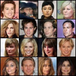
Figure 10: Image Generations (Top). Figure 11: Generations. GEM (right) produces reasonable samples
GEM (right) generates comparable im- across the shape and audiovisual modalities. In contrast, audiovisual
ages to FDN. Nearest Neighbors (Bot- generations from StyleGAN2 exhibit noise, while FDN generates
tom). Illustration of nearest neighbors poor samples in both modalities.
in latent space of generations.
observe that GEM is able to generate empty spectograms when the bow is not on the cello, as well as
different spectrograms dependent on the position of the bow. Alternatively, in Figure 8, we provide
only an input audio spectrogram and ask GEM to generate possible images. In this setting, we find
that generated images have the bow off the cello when the input spectrogram is empty (with the bow
missing due to GEM blurring the uncertainty of all possible locations of the bow), and at different
positions depending on the input audio spectrogram. In contrast, we found that all baselines were
unable to fit the audiovisual setting well, as discussed in Section 5.1 and shown in Figure 11.
5.3 Generating Data Samples
Finally, we investigate the ability of GEM to generate new data samples.
Qualitative Generations. We show random samples drawn from GEM and compare these to
our baselines. We consider images in Figure 10, shapes in Figure 11, audio snippets in Figure 9
and audiovisual inputs in Figure 11. While we find that GEM performs comparably to FDN in
the image regime, our model significantly outperforms all baselines on domains of audio, shape,
and audiovisual modalities. We further display nearest latent space neighbors of generations on
CelebA-HQ in Figure 10 and find that our generations are distinct from those in the training dataset.
Quantitative Comparisons. Next, we provide quantitiative evaluations of generations in Table 2
on image and shape modalities. We report the FID [44], precision, and recall [45] metrics on CelebA-
HQ 64 × 64. We find that GEM performs better than StyleGAN2 and FDN on precision and recall,
but worse in terms of FID. We note that our qualitative generations in Figure 10 are comparable
to those of FDN; however, we find that our approach obtains high FID scores due to the inherent
sensitivity of the FID metric to blur. Such sensitivity to bluriness has also been noted in [46], and we
9find that even our autodecoded training distribution obtains an FID of 23.25, despite images appearing
near perceptually perfect (Figure 3). On ShapeNet, we report coverage and MMD metrics from [47]
using Chamfer Distance. To evaluate generations, we sample 8762 shapes (the size of test Shapenet
dataset) and generate 2048 points following [40]. We compare generations from GEM with those
of FDN and latent GAN trained on IMNET (using the provided code in [40]). We find that GEM
outperforms both approaches on the task of 3D shape generation.
6 Conclusion
We have presented GEM, an approach to learn a modality-independent manifold. We demonstrate how
our model enables us to interpolate between signals, complete partial signals, and further generate
new signals. A limitation of our approach is that while underlying manifolds are recovered, they are
not captured with high-fidelity. We believe that a promising direction of future work involves the
pursuit of further engineered inductive biases, and general structure, which enable the recovery of
high-fidelity manifolds of the plethora of signals in the world around us. We emphasize, however,
that as our manifold is constructed over a dataset; GEM may learn to incorporate and propogate
existing prejudices and biases present in such data, posing risks for mass deployment of our model.
Additionally, while our work offers exciting avenues for cross-modal modeling and generation, we
note that GEM has the potential to be used to create enhanced "deep fakes" and other forms of
synthetic media.
Acknowledgements This project is supported by DARPA under CW3031624 (Transfer, Augmen-
tation and Automatic Learning with Less Labels), the Singapore DSTA under DST00OECI20300823
(New Representations for Vision), as well as ONR MURI under N00014-18-1-2846. We would like
to thank Bill Freeman and Fredo Durand for giving helpful comments on the manuscript. Yilun Du is
supported by an NSF graduate research fellowship.
References
[1] Sebastian H. Seung and Daniel Lee. The manifold ways of perception. Science, 290:2268–2269, 2000. 1
[2] Joshua B Tenenbaum, Vin De Silva, and John C Langford. A global geometric framework for nonlinear
dimensionality reduction. Sci., 290(5500):2319–2323, 2000. 1, 2, 4
[3] Sam T Roweis and Lawrence K Saul. Nonlinear dimensionality reduction by locally linear embedding.
Sci., 290(5500):2323–2326, 2000. 1, 2, 4
[4] Ian Goodfellow, Jean Pouget-Abadie, Mehdi Mirza, Bing Xu, David Warde-Farley, Sherjil Ozair, Aaron
Courville, and Yoshua Bengio. Generative adversarial nets. In NeurIPS, 2014. 1, 3, 4
[5] David Ha, Andrew Dai, and Quoc V Le. Hypernetworks. In Proc. ICLR, 2017. 2
[6] Bernhard Schölkopf, Alexander J. Smola, and Klaus-Robert Müller. Nonlinear component analysis as a
kernel eigenvalue problem. Neural Comput., 10(5):1299–1319, 1998. 2
[7] Mikhail Belkin and Partha Niyogi. Laplacian eigenmaps for dimensionality reduction and data representa-
tion. Neural Comput., 15(6):1373–1396, June 2003. 2
[8] Ronald R. Coifman and Stéphane Lafon. Diffusion maps. Applied and Computational Harmonic Analysis,
21(1):5–30, 2006. Special Issue: Diffusion Maps and Wavelets.
[9] David L. Donoho and Carrie Grimes. Hessian eigenmaps: Locally linear embedding techniques for
high-dimensional data. Proceedings of the National Academy of Sciences, 100(10):5591–5596, 2003.
[10] Laurens van der Maaten and Geoffrey Hinton. Visualizing data using t-SNE. Journal of Machine Learning
Research, 9:2579–2605, 2008. 2
[11] Kui Jia, Lin Sun, Shenghua Gao, Zhan Song, and Bertram E. Shi. Laplacian auto-encoders: An explicit
learning of nonlinear data manifold. Neurocomputing, 160:250–260, 2015. 2
[12] Gal Mishne, Uri Shaham, Alexander Cloninger, and Israel Cohen. Diffusion nets. Applied and Computa-
tional Harmonic Analysis, 47(2):259–285, 2019.
[13] Gautam Pai, Ronen Talmon, Alex Bronstein, and Ron Kimmel. Dimal: Deep isometric manifold learning
using sparse geodesic sampling, 2018. 2
[14] Yufan Zhou, Changyou Chen, and Jinhui Xu. Learning manifold implicitly via explicit heat-kernel learning.
arXiv preprint arXiv:2010.01761, 2020. 2, 6
10[15] Kyle Genova, Forrester Cole, Daniel Vlasic, Aaron Sarna, William T Freeman, and Thomas Funkhouser.
Learning shape templates with structured implicit functions. In Proc. ICCV, pages 7154–7164, 2019. 3
[16] Kyle Genova, Forrester Cole, Avneesh Sud, Aaron Sarna, and Thomas Funkhouser. Deep structured
implicit functions. arXiv preprint arXiv:1912.06126, 2019. 3
[17] Jeong Joon Park, Peter Florence, Julian Straub, Richard Newcombe, and Steven Lovegrove. Deepsdf:
Learning continuous signed distance functions for shape representation. In Proc. CVPR, 2019. 3, 4
[18] Mateusz Michalkiewicz, Jhony K Pontes, Dominic Jack, Mahsa Baktashmotlagh, and Anders Eriksson.
Implicit surface representations as layers in neural networks. In Proc. ICCV, pages 4743–4752, 2019.
[19] Matan Atzmon and Yaron Lipman. Sal: Sign agnostic learning of shapes from raw data. In Proc. CVPR,
2020.
[20] Amos Gropp, Lior Yariv, Niv Haim, Matan Atzmon, and Yaron Lipman. Implicit geometric regularization
for learning shapes. In Proc. ICML, 2020. 3
[21] Vincent Sitzmann, Michael Zollhöfer, and Gordon Wetzstein. Scene representation networks: Continuous
3d-structure-aware neural scene representations. In Proc. NeurIPS 2019, 2019. 3, 4
[22] Chiyu Jiang, Avneesh Sud, Ameesh Makadia, Jingwei Huang, Matthias Nießner, and Thomas Funkhouser.
Local implicit grid representations for 3d scenes. In Proc. CVPR, pages 6001–6010, 2020.
[23] Songyou Peng, Michael Niemeyer, Lars Mescheder, Marc Pollefeys, and Andreas Geiger. Convolutional
occupancy networks. In Proc. ECCV, 2020.
[24] Rohan Chabra, Jan Eric Lenssen, Eddy Ilg, Tanner Schmidt, Julian Straub, Steven Lovegrove, and Richard
Newcombe. Deep local shapes: Learning local sdf priors for detailed 3d reconstruction. arXiv preprint
arXiv:2003.10983, 2020. 3
[25] Vincent Sitzmann, Julien N. P. Martel, Alexander W. Bergman, David B. Lindell, and Gordon Wetzstein.
Implicit neural representations with periodic activation functions, 2020. 3
[26] Lars Mescheder, Michael Oechsle, Michael Niemeyer, Sebastian Nowozin, and Andreas Geiger. Occupancy
networks: Learning 3d reconstruction in function space. In Proc. CVPR, 2019. 3
[27] Vincent Sitzmann, Eric R Chan, Richard Tucker, Noah Snavely, and Gordon Wetzstein. Metasdf: Meta-
learning signed distance functions. Proc. NeurIPS, 2020. 3
[28] Eric R Chan, Marco Monteiro, Petr Kellnhofer, Jiajun Wu, and Gordon Wetzstein. pi-gan: Periodic implicit
generative adversarial networks for 3d-aware image synthesis. Proc. CVPR, 2020. 3
[29] Katja Schwarz, Yiyi Liao, Michael Niemeyer, and Andreas Geiger. Graf: Generative radiance fields for
3d-aware image synthesis. Proc. NeurIPS, 2020. 3
[30] Emilien Dupont, Yee Whye Teh, and Arnaud Doucet. Generative models as distributions of functions.
arXiv preprint arXiv:2102.04776, 2021. 3, 6, 9, 13
[31] Tero Karras, Samuli Laine, Miika Aittala, Janne Hellsten, Jaakko Lehtinen, and Timo Aila. Analyzing and
improving the image quality of stylegan. In Proceedings of the IEEE/CVF Conference on Computer Vision
and Pattern Recognition (CVPR), June 2020. 3, 6, 13
[32] Chris Donahue, Julian McAuley, and Miller Puckette. Adversarial audio synthesis, 2019. 3, 6
[33] Diederik P Kingma, Shakir Mohamed, Danilo Jimenez Rezende, and Max Welling. Semi-supervised
learning with deep generative models. In NeurIPS, 2014. 3
[34] Aaron van den Oord, Nal Kalchbrenner, and Koray Kavukcuoglu. Pixel recurrent neural networks. Proc.
ICML, 2016. 3
[35] Aaron van den Oord, Sander Dieleman, Heiga Zen, Karen Simonyan, Oriol Vinyals, Alex Graves, Nal
Kalchbrenner, Andrew Senior, and Koray Kavukcuoglu. Wavenet: A generative model for raw audio, 2016.
3
[36] Aditya Ramesh, Mikhail Pavlov, Gabriel Goh, Scott Gray, Chelsea Voss, Alec Radford, Mark Chen, and
Ilya Sutskever. Zero-shot text-to-image generation, 2021. 3
[37] Ivan Skorokhodov, Savva Ignatyev, and Mohamed Elhoseiny. Adversarial generation of continuous images.
arXiv preprint arXiv:2011.12026, 2020. 3, 13
[38] Tero Karras, Timo Aila, Samuli Laine, and Jaakko Lehtinen. Progressive growing of gans for improved
quality, stability, and variation. In ICLR, 2017. 6
[39] Jesse Engel, Cinjon Resnick, Adam Roberts, Sander Dieleman, Douglas Eck, Karen Simonyan, and
Mohammad Norouzi. Neural audio synthesis of musical notes with wavenet autoencoders, 2017. 6
[40] Zhiqin Chen and Hao Zhang. Learning implicit fields for generative shape modeling. In Proc. CVPR,
pages 5939–5948, 2019. 6, 9, 10
11[41] Lele Chen, Sudhanshu Srivastava, Zhiyao Duan, and Chenliang Xu. Deep cross-modal audio-visual
generation, 2017. 6
[42] Diederik P. Kingma and Max Welling. Auto-encoding variational bayes. In ICLR, 2014. 6
[43] Laurens Van der Maaten and Geoffrey Hinton. Visualizing data using t-sne. JMLR, 9(11):2579–2605,
2008. 7
[44] Martin Heusel, Hubert Ramsauer, Thomas Unterthiner, Bernhard Nessler, and Sepp Hochreiter. Gans
trained by a two time-scale update rule converge to a local nash equilibrium. In Advances in Neural
Information Processing Systems, pages 6626–6637, 2017. 9
[45] Tuomas Kynkäänniemi, Tero Karras, Samuli Laine, Jaakko Lehtinen, and Timo Aila. Improved precision
and recall metric for assessing generative models. CoRR, abs/1904.06991, 2019. 9
[46] Ali Razavi, Aaron van den Oord, and Oriol Vinyals. Generating diverse high-fidelity images with vq-vae-2,
2019. 9
[47] Panos Achlioptas, Olga Diamanti, Ioannis Mitliagkas, and Leonidas J Guibas. Learning representations
and generative models for 3d point clouds. arXiv preprint arXiv:1707.02392, 2017. 10
[48] Diederik P. Kingma and Jimmy Ba. Adam: A method for stochastic optimization. In ICLR, 2015. 13
[49] Ben Mildenhall, Pratul P Srinivasan, Matthew Tancik, Jonathan T Barron, Ravi Ramamoorthi, and Ren Ng.
Nerf: Representing scenes as neural radiance fields for view synthesis. In Proc. ECCV, 2020. 14
12A.1 Appendix for Learning Signal-Agnostic Manifolds of Neural Fields
Please visit our project website at https://yilundu.github.io/gem/ for additional qualitative
visualizations of test-time reconstruction of audio and audiovisual samples, traversals along the
underlying manifold of GEM on CelebA-HQ as well as interpolations between audio samples. We
further illustrate additional image in-painting results, as well as audio completion results. Finally, we
visualize several audio and audiovisual generations.
In Section A.1.1 below, we provide details on training settings, as well as the underlying baseline
model architectures utilized for each modality. We conclude with details on reproducing our work in
Section A.1.2.
A.1.1 Experimental Details
Training Details For each separate training modality, all models and baselines are trained for one
day, using one 32GB Volta machine. GEM is trained with the Adam optimizer [48], using a training
batch size of 128 and a learning rate of 1e-4. Each individual datapoint is fit by fitting the value of
1024 sampled points in the sample (1024 for each modality in the multi-modal setting). We normalize
the values of a signals to be between -1 and 1. When computing LIso , a scalar constant of α = 100 is
employed to scale distances in the underlying manifold to that of distances of signals in sample space.
When enforcing LLLE , a total of 10 neighbors are considered to compute the loss across modalities.
We utilize equal loss weight across LRec , LIso , LLLE , and found that the relative magnitudes of each
loss had little impact on the overall performance.
Model Details We provide the architectures of the hypernetwork ψ and implicit function φ utilized
by GEM across separate modalities in Table 4 and Table 5, respectively. Additionally, we provide the
architectures used in each domain for our baselines: StyleGAN2 in Table 15 each domain in Table 15
and VAE in Table 10. Note that for the VAE, the ReLU nonlinearity is used, with each separate
convolution having stride 2.
We obtained the hyperparameters for implicit functions and hypernetworks based off of [37]. Early in
the implementation of the project, we explored a variety of additional architectural choices; however,
we ultimately found that neither changing the number of layers in the hypernetworks, nor changing
the number of underlying hidden units in networks, significantly impacted the performance of GEM.
We will add these details to the appendix of the paper.
A.1.2 Reproducibility
We next describe details necessary to reproduce each of other underlying empirical results.
Hyperparameter Settings for Baselines We employ the default hyperparameters, as used in the
original papers for StyleGAN2 [31] and FDN [30], to obtain state-of-the-art performance on their
respective tasks. Due to computational constraints, we were unfortunately unable to do a complete
hyperparameter search for each method over all tasks considered. Despite this, we were able to run
the models on toy datasets and found that these default hyperparameters performed the best. We
utilized the author’s original codebases for experiments.
Variance Across Seeds Results in the main tables of the paper are run across a single evaluated
seed. Below in Table 3, we rerun test reconstruction results on CelebA-HQ across different models
utilizing a total of 3 separate seeds. We find minimal variance across separate runs, and still find the
GEM performs significantly outperforms baselines.
Modality Model MSE ↓ PSNR ↑
VAE 0.0327 ± 0.0035 15.16 ± 0.06
FDN 0.0062 ± 0.0003 22.57 ± 0.02
Images
StyleGANv2 0.0044 ± 0.0001 24.03 ± 0.01
GEM 0.0025 ± 0.0001 26.53 ± 0.01
Table 3: Test CelebA-HQ reconstruction results of different methods evaluated across 3 different seeds. We
further report standard deviation between different runs.
13Datasets We provide source locations to download each of the datasets we used in the paper.
The CelebA-HQ dataset can be downloaded at https://github.com/tkarras/progressive_
growing_of_gans/blob/master/dataset_tool.py and is released under the Creative Com-
mons license. The NSynth dataset may be downloaded at https://magenta.tensorflow.
org/datasets/nsynth and is released under the Creative Commons license. The ShapeNet
dataset can be downloaded at https://github.com/czq142857/IM-NET and is released un-
der the MIT License, and finally the Sub-URMP dataset we used may be downloaded at https:
//www.cs.rochester.edu/~cxu22/d/vagan/.
Pos Embed (512)
Dense → 512 Dense → 512
Dense → 512 Dense → 512
Dense → 512 Dense → 512
Dense → φ Parameters Dense → Output Dim
Table 4: The architecture of the hypernetwork uti- Table 5: The architecture of the implicit function
lized by GEM. φ used to agnostically encode each modality. We
utilize the Fourier embedding from [49] to embed
coordinates.
3x3 Conv2d, 32
3x3 Conv2d, 32
3x3 Conv2d, 64
3x3 Conv2d, 64
3x3 Conv2d, 32 3x3 Conv2d, 128
3x3 Conv2d, 128
3x3 Conv2d, 64 3x3 Conv2d, 64 3x3 Conv2d, 256
3x3 Conv2d, 256
3x3 Conv2d, 128 3x3 Conv2d, 128 3x3 Conv2d, 512
3x3 Conv2d, 512
3x3 Conv2d, 256 3x3 Conv2d, 256 z ← Encode
z ← Encode
3x3 Conv2d, 512 3x3 Conv2d, 512 Reshape(4, 1)
Reshape(2, 2)
3x3 Conv2d, 512 z ← Encode 3x3 Conv2d Transpose, 512
3x3 Conv2d Transpose, 512
z ← Encode Reshape(4, 2) 3x3 Conv2d Transpose, 256
3x3 Conv2d Transpose, 256
Reshape(2, 2) 3x3 Conv2d Transpose, 512 3x3 Conv2d Transpose, 128
3x3 Conv2d Transpose, 128
3x3 Conv2d Transpose, 512 3x3 Conv2d Transpose, 256 3x3 Conv2d Transpose, 64
3x3 Conv2d Transpose, 64
3x3 Conv2d Transpose, 512 3x3 Conv2d Transpose, 128 3x3 Conv2d Transpose, 32
3x3 Conv2d Transpose, 32
3x3 Conv2d Transpose, 256 3x3 Conv2d Transpose, 64 3x3 Conv2d Transpose, 1
3x3 Conv2d Transpose, 3
3x3 Conv2d Transpose, 128 3x3 Conv2d Transpose, 32 Crop
3x3 Conv2d Transpose, 3 3x3 Conv2d Transpose, 1 Table 8: The architecture
of encoder and decoder Table 9: The architecture
Crop of encoder and decoder
Table 6: The encoder of the VAE utilized for
and decoder of the VAE audiovisual dataset on of the VAE utilized for
Table 7: The encoder
utilized for CelebA-HQ. images. Latent encod- audiovisual dataset on
and decoder of the VAE
ings from image and au- audio. Latent encodings
utilized for NSynth
dio modalities are added from image and audio
together. modalities are added to-
gether.
Table 10: The architecture of the VAE utilized across datasets.
14Constant Input (512, 8, 2)
Constant Input (512, 8, 4) Constant Input (512, 4, 4)
Constant Input (512, 4, 4) StyleConv 512
StyleConv 512 StyleConv 512
StyleConv 512 StyleConv 512
StyleConv 512 StyleConv 512
StyleConv 512 StyleConv 512
StyleConv 512 StyleConv 512
StyleConv 512 StyleConv 512
StyleConv 512 StyleConv 512
StyleConv 512 StyleConv 256
StyleConv 256 StyleConv 256
StyleConv 256 3x3 Conv2d, 1
3x3 Conv2d, 1 3x3 Conv2d, 3
3x3 Conv2d, 3 Crop
Crop
Table 13: The genera-
Table 11: The genera- Table 14: The genera-
Table 12: The genera- tor architecture of Style-
tor architecture of Style- tor architecture of Style-
tor architecture of Style- GAN2 for audiovisual
GAN2 for CelebA-HQ. GAN2 for audiovisual
GAN2 for NSynth domain for images.
domain for audio.
Table 15: The architecture of the StyleGAN generator utilized across datasets.
15You can also read