Time of emergence of compound events: contribution of univariate and dependence properties - NHESS
←
→
Page content transcription
If your browser does not render page correctly, please read the page content below

Nat. Hazards Earth Syst. Sci., 23, 21–44, 2023
https://doi.org/10.5194/nhess-23-21-2023
© Author(s) 2023. This work is distributed under
the Creative Commons Attribution 4.0 License.

Time of emergence of compound events: contribution
of univariate and dependence properties
Bastien François and Mathieu Vrac
Laboratoire des Sciences du Climat et l’Environnement (LSCE-IPSL) CNRS/CEA/UVSQ,
UMR8212, Université Paris-Saclay, Gif-sur-Yvette, France

Correspondence: B. François (bastien.francois@lsce.ipsl.fr)

Received: 26 April 2022 – Discussion started: 9 May 2022
Revised: 3 November 2022 – Accepted: 12 December 2022 – Published: 11 January 2023

Abstract. Many climate-related disasters often result from          ity changes. These results highlight the importance of con-
a combination of several climate phenomena, also referred           sidering changes in both marginal and dependence proper-
to as “compound events’’ (CEs). By interacting with each            ties, as well as their inter-model variability, for future risk
other, these phenomena can lead to huge environmental and           assessments related to CEs.
societal impacts, at a scale potentially far greater than any of
these climate events could have caused separately. Marginal
and dependence properties of the climate phenomena form-
ing the CEs are key statistical properties characterising their     1   Introduction
probabilities of occurrence. In this study, we propose a new
methodology to assess the time of emergence of CE proba-            In September 2017, heavy rainfall and storm surge associ-
bilities, which is critical for mitigation strategies and adapta-   ated with Hurricane Irma resulted in record-breaking floods
tion planning. Using copula theory, we separate and quantify        in Jacksonville, Florida. In 2019, Australia experienced high
the contribution of marginal and dependence properties to the       temperatures and prolonged dry conditions, which resulted
overall probability changes of multivariate hazards leading to      in one of the worst bush fire seasons in its recorded history.
CEs. It provides a better understanding of how the statistical      In April 2021 and 2022, Central Europe experienced con-
properties of variables leading to CEs evolve and contribute        secutive days of frost events following a warm early spring,
to the change in their occurrences. For illustrative purposes,      which caused severe damage to agricultural yields. These
the methodology is applied over a 13-member multi-model             recent climate events are some examples of so-called com-
ensemble (CMIP6) to two case studies: compound wind and             pound events (CEs), i.e. high-impact climate events that re-
precipitation extremes over the region of Brittany (France),        sult from interactions of several climate hazards. These cli-
and frost events occurring during the growing season precon-        mate hazards are not necessarily extremes themselves, but
ditioned by warm temperatures (growing-period frost) over           their simultaneous or successive occurrences can generate
central France. For compound wind and precipitation ex-             strong impacts (Leonard et al., 2014; Zscheischler et al.,
tremes, results show that probabilities emerge before the end       2014, 2018, 2020). Although still in its infancy, the un-
of the 21st century for six models of the CMIP6 ensemble            derstanding of the complex nature of CEs and the assess-
considered. For growing-period frosts, significant changes          ment of their associated risks have been the subject of nu-
of probability are detected for 11 models. Yet, the contribu-       merous research studies in climate sciences (e.g. Bevacqua
tion of marginal and dependence properties to these changes         et al., 2017, 2021; Manning et al., 2018; Zscheischler and
in probabilities can be very different from one climate haz-        Seneviratne, 2017; Ridder et al., 2021, 2022; Singh et al.,
ard to another, and from one model to another. Depending            2021a; Nasr et al., 2021; Raymond et al., 2022, among
on the CE, some models place strong importance on both              many others). Recently, a typology of CEs has been pro-
marginal properties and dependence properties for probabil-         posed in order to categorise them into four classes depend-
                                                                    ing on how individual hazards interact to form the CEs

Published by Copernicus Publications on behalf of the European Geosciences Union.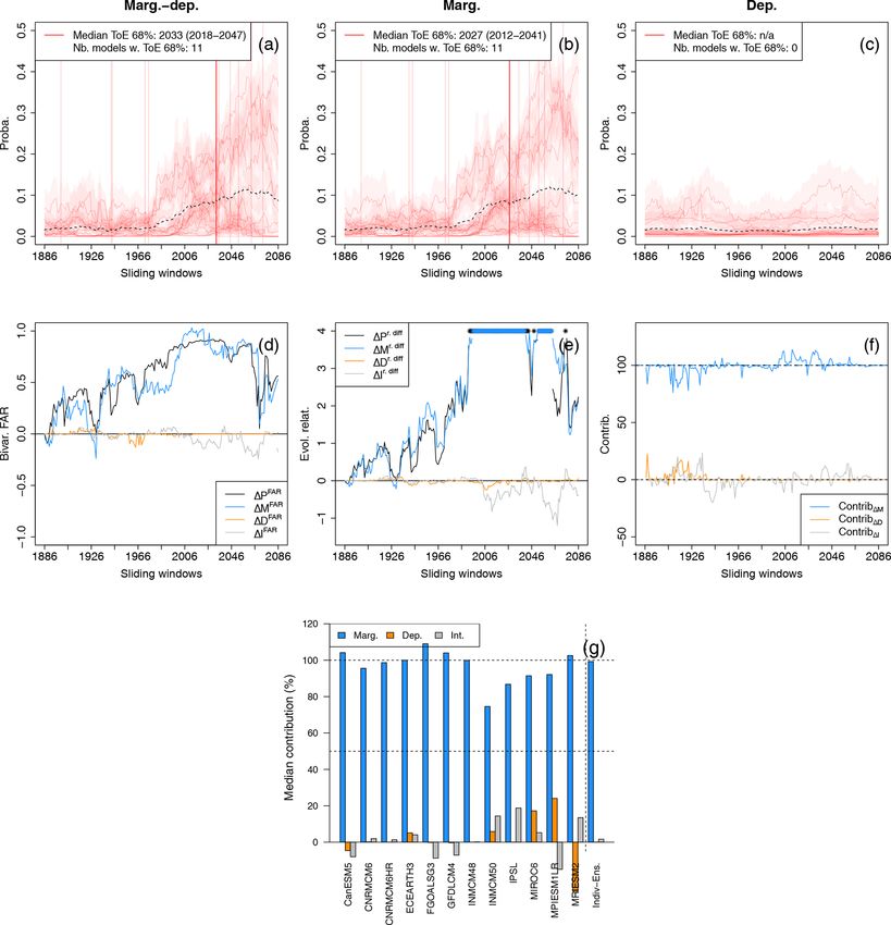
22                                                         B. François and M. Vrac: Time of emergence of compound events

(“preconditioned”, “multivariate’’, “temporally compound-          also combine to change the probabilities of the CE hazards
ing’’ and “spatially compounding’’ events; see Zscheischler        (e.g. Rana et al., 2017; Zscheischler and Seneviratne, 2017;
et al., 2020). Concerning projected changes, the frequency         Zscheischler and Lehner, 2021; Manning et al., 2019; Singh
and intensity of some CEs such as co-occurring heatwaves           et al., 2021a). For example, rising temperatures can naturally
and droughts are expected to increase for many regions of          lead to more co-occurrences of hot temperatures and mete-
the world, even when considering climate change scenarios          orological droughts, despite no significant trends in meteo-
with limited global warming to 1.5 ◦ C above pre-industrial        rological droughts being detected (Diffenbaugh et al., 2015;
levels (IPCC, 2023). Determining whether the probabilities         Mazdiyasni and AghaKouchak, 2015). However, in addition
of compounding climate events present significant changes          to warmer temperatures, the strengthening of the dependence
between past and future periods and detecting when these           between hot temperatures and meteorological droughts for
significant changes occur are of paramount importance, not         future periods can also contribute to an increase in their
only for mitigation and adaptation issues but also for in-         co-occurrences (as highlighted in Zscheischler and Senevi-
forming the general public and raising awareness of climate        ratne, 2017). Several studies concluded on the importance of
change. Only when the changes of probability are of suffi-         considering dependencies to assess CE properties and fre-
cient magnitude relative to a baseline period can we be con-       quencies in a robust way, e.g. for wind and precipitation
fident that significant changes have been detected. Detecting      extremes (e.g. Hillier et al., 2020), or temperature and pre-
from which period the changes are statistically significant        cipitation (e.g. Singh et al., 2021a; Vrac et al., 2022a). Re-
corresponds to the concept of “time of emergence” (ToE).           cently, Abatzoglou et al. (2020) even showed that, in recent
It consists in determining the time or period in which a cli-      decades, changes in multivariate annual climatic conditions
mate signal emerges from (i.e. goes out of) the natural vari-      (water deficit, evapotranspiration, minimum and maximum
ability (e.g. Christensen et al., 2007; Maraun, 2013; Hawkins      temperature) with respect to a reference climate state have
et al., 2020; Ossó et al., 2022). ToE has been discussed exten-    been more important than changes in univariate annual cli-
sively to analyse the emergence of mean temperatures (e.g.         matic conditions for a large portion of the Earth. Hence, to
Hawkins and Sutton, 2012; Mahlstein et al., 2011), precipita-      determine the ToE of hazard probabilities, quantifying the
tion (Fischer et al., 2014; Giorgi and Bi, 2009; Gaetani et al.,   influence (or contribution) of the statistical features of the
2020), but also emergence of extremes (e.g. Diffenbaugh and        variables forming the CEs on these changes of probabilities
Scherer, 2011; Fischer et al., 2014; King et al., 2015). Evalu-    is crucial in order to further understand the potential future
ating the ToE of compound hazard probabilities with respect        evolution of CEs (Vrac et al., 2022a).
to a baseline period – from which the natural variability is es-      In this paper, we propose a new methodology to assess
timated – is valuable for the analysis of the evolution of CEs     the ToE of CE probabilities. We also develop a copula-based
and for attributing this to a specific cause, such as anthro-      multivariate framework, which allows for an adequate de-
pogenic greenhouse gas emissions. Detection and attribu-           scription of the contribution of the changes in marginal and
tion represent an important research field in climate science      dependence properties to the evolution of multivariate hazard
that aims to determine the mechanisms responsible for re-          probabilities. This CE analysis is applied to two case stud-
cent global warming and related climate changes (e.g. Bind-        ies. Please note that the goal of the paper is not to provide
off et al., 2013). For example, it can be done by comparing        precise results of ToE in these two case studies, but rather
probabilities of an event between two worlds with different        to introduce the conceptual framework and raise awareness
forcings (the “risk-based” approach; Stott et al., 2004; Shep-     among climate scientists on the potential emergence of CE
herd, 2016). Generally, a factual world with anthropogenic         probabilities, as well as the contributions of statistical proper-
climate change and a counterfactual world in which anthro-         ties to probability changes. We first analyse compound wind
pogenic emissions had never occurred are considered. Al-           and precipitation extremes over the coastal region of Brittany
though we do not aim at performing attribution per se in the       (France). This bivariate CE, i.e. composed of co-occurring
present study, the underlying philosophy is relatively similar     climate hazards over the same region and time, has been anal-
for ToE: by considering a pre-industrial period as baseline,       ysed in several studies (e.g. Martius et al., 2016; Bevacqua
compound hazard probabilities associated with natural forc-        et al., 2019; De Luca et al., 2020a; Reinert et al., 2021; Mess-
ings – or natural variability – may be estimated, and thus also    mer and Simmonds, 2021) as it can have severe impacts such
the influence of future climate change on probabilities.           as important economic losses, massive damage to infrastruc-
   From a statistical point of view, CEs are characterised by      ture and loss of human life (e.g. Fink et al., 2009; Liberato,
the statistical features of the variables forming the CEs, i.e.    2014; Wahl et al., 2015; Raveh-Rubin and Wernli, 2015). We
their marginal properties (e.g. mean and variance) and depen-      then apply our methodology to a second climate hazard: frost
dence structures. These key statistical properties can be af-      events occurring during the growing season preconditioned
fected by future climate change (e.g. Wahl et al., 2015; Schär,    by warm temperatures (growing-period frost) over central
2015; Russo et al., 2017; Raymond et al., 2020; Jézéquel           France. When occurring after bud burst, i.e. when the sen-
et al., 2020). In addition to potentially exacerbating impacts,    sitive emerging leaves and flowers have started to develop,
these changes in marginal and dependence properties could          frost temperatures potentially affect the growth and distri-

Nat. Hazards Earth Syst. Sci., 23, 21–44, 2023                                        https://doi.org/10.5194/nhess-23-21-2023
B. François and M. Vrac: Time of emergence of compound events                                                                  23

bution limits of plants. It can consequently cause important      wind and precipitations extremes is therefore relevant for this
economic losses to agriculture (Lamichhane, 2021). These          region. To allow for a robust statistical modelling of com-
growing-period frost events and their associated risks in past    pounding wind and precipitation extremes, we applied our
and future periods have been studied in the literature (e.g.      methodology to bivariate points of high values by selecting
Unterberger et al., 2018; Liu et al., 2018a; Sgubin et al.,       wind and precipitation data concurrently exceeding selected
2018; Pfleiderer et al., 2019), as has the role of human-caused   high thresholds. Indeed, our methodology detailed later in
climate change in growing-period frost probability (Vautard       Sect. 3 is based on the use of parametric models, and consid-
et al., 2022).                                                    ering the complete bivariate distribution to fit marginals and
   The rest of this paper is organised as follows: Sect. 2 de-    copulas may not be appropriate as the representation of the
scribes the climate simulations used in this study, and Sect. 3   extremes would be biased by the bulk of the bivariate dis-
details the statistical method and experimental setup used to     tributions where most of the data are located (e.g. Bevacqua
analyse the ToE of CE probabilities and the contributions of      et al., 2019). More details on selection thresholds are pro-
the statistical features. The results from the analysis of the    vided in Sect. 4.
two climate compound hazards are provided in Sect. 4 for ex-         For growing-period frost events, data are extracted over
tremes of wind and precipitation and in Sect. 5 for growing-      central France ([−1, 5◦ E] × [46, 49◦ N], see Fig. 1a), which
period frost events. Conclusions, discussions and perspec-        corresponds to 78 continental grid cells. The region covers
tives for future research are finally proposed in Sect. 6.        an important agriculture area of France, including grapevine
                                                                  and fruit crops with high production (Vautard et al., 2022).
                                                                  We focus on the spatial mean of daily minimum temperature
2   Model data                                                    (T ) in April to define frost events occurring in early spring.
                                                                  To account for phenology and to characterise bud burst con-
One ensemble of 13 global climate models (GCMs) follow-           ditions by the end of March, the growing degree day (GDD)
ing the CMIP6 protocol (Eyring et al., 2016) is considered.       model (Bonhomme, 2000) is used. The GDD model consists
This selection of models is listed in Table 1. To define com-     in computing cumulative daily mean temperatures minus a
pound wind and precipitation extremes, we use daily pre-          “base temperature” from a starting date. For our study, a base
cipitation and wind speed maxima variables. For growing-          temperature of 5 ◦ C is used and the starting date for comput-
period frost, mean and minimum temperature variables are          ing GDD values for each year is chosen to be 1 January. In
used. For each variable, the historical period simulations        this study, our aim is not to focus on the phenology of specific
(1871–2014) have been extracted and extended until 2100 us-       plants but rather to provide a general overview of growing-
ing the shared socioeconomic pathways 585 (SSP-585) sce-          period frost events. Generally, 5 ◦ C as base temperature is
nario (Riahi et al., 2017). Since the 13 selected simulations     accepted for crops and grapevine (e.g. Skaugen and Tveito,
present different spatial resolutions, each climate simulation    2004; Jiang et al., 2011; Ruosteenoja et al., 2016; Vautard
dataset has been regridded to a common spatial resolution of      et al., 2022). Bud burst occurs when the cumulative sum of
0.5◦ × 0.5◦ using bilinear interpolation. Considering the cli-    degree-days up to 31 March is larger than some thresholds
mate models separately will allow us to assess inter-model        (Garcia de Cortazar-Atauri et al., 2009) which depend on
variability in terms of ToE of CE probabilities, as well as       species. For each year y, GDD values by the end of March
the potentially different contributions of marginal and de-       are obtained via the formula
pendence properties to changes in probability of multivari-                    i=y/03/31
ate climate hazards. Also, by considering all climate models      GDD(y) :=
                                                                                 X
                                                                                           max(MT(i) − 5, 0),
together using a pooling procedure, a multi-model ensemble                     i=y/01/01
estimate for ToE and contributions may be derived. Pooling
the models together will allow us better to take into account     with MT the daily mean temperature. GDD values are com-
the global uncertainty inherent in climate modelling and to       puted for each grid cell and averaged spatially over the area
reduce the influence of natural variability amongst individ-      of central France. We consider the threshold of 200 ◦ C.day to
ual ensemble members.                                             characterise bud burst conditions and illustrate our method.
   For compounding wind and precipitation extremes, we use        The choice of this threshold is consistent with existing stud-
the spatial mean of daily wind speed maxima and the spa-          ies analysing bud burst values of grapevine species (e.g. Gar-
tial sum of daily precipitation time series during winter (De-    cia de Cortazar-Atauri et al., 2009; Vautard et al., 2022), and
cember, January and February) over the region of Brittany,        is useful for characterising early bud burst plants that could
France ([−5, −2◦ E] × [46.5, 49◦ N], see Fig. 1a), which cor-     be impacted by frost events.
responds to a domain with 21 continental grid cells in our           For illustrative purposes, Fig. 1a displays the topographic
regridded climate simulations. This coastal region is regu-       map of France with the region of Brittany and central France
larly impacted by mid-latitude extra-tropical storms causing      in boxes. The bivariate wind and precipitation data (Fig. 1b)
significant damage to infrastructures (e.g. storm Xynthia in      and minimal temperature and GDD data (Fig. 1c) for the
2010). Analysing the evolution of probability of compound         CNRM-CM6 model are also displayed.

https://doi.org/10.5194/nhess-23-21-2023                                      Nat. Hazards Earth Syst. Sci., 23, 21–44, 2023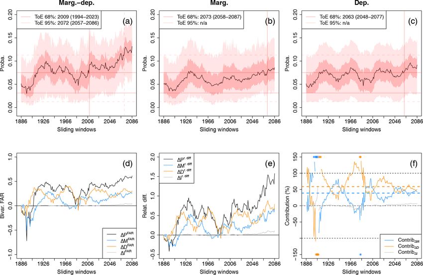
24                                                            B. François and M. Vrac: Time of emergence of compound events

Table 1. List of CMIP6 simulations used in this study, their run, approximate horizontal resolution and references.

    Model               Institution                                                                   Spatial res.    Data reference
                                                                                                    (long. × lat.)
    CanESM5             Canadian Centre for Climate Modelling and Analysis, Canada                2.81◦ × 2.81◦       Swart et al. (2019)
    FGOALS-g3           Chinese Academy of Sciences, China                                        2.00◦ × 2.25◦       Li (2019)
    CNRM-CM6-1          Centre National de Recherches Meteorologiques, Meteo-France, France       1.41◦ × 1.41◦       Voldoire (2019)
    CNRM-CM6-1-HR       Centre National de Recherches Meteorologiques, Meteo-France, France       0.50◦ × 0.50◦       Voldoire (2018)
    GFDL-CM4            Geophysical Fluid Dynamics Laboratory, USA                                   1.25◦ × 1◦       Guo et al. (2018)
    INM-CM4-8           Institute for Numerical Mathematics, Russia                                   2◦ × 1.5◦       Volodin et al. (2019a)
    INM-CM5-0           Institute for Numerical Mathematics, Russia                                   2◦ × 1.5◦       Volodin et al. (2019b)
    IPSL-CM6A-LR        Institut Pierre-Simon Laplace, France                                     2.50◦ × 1.26◦       Boucher et al. (2018)
    MIROC6              JAMSTEC, AORI, NIES, R-CCS, Japan                                         1.41◦ × 1.41◦       Shiogama et al. (2019)
    MPI-ESM1-2-LR       Max Planck Institute for Meteorology, Germany                             1.88◦ × 1.88◦       Wieners et al. (2019)
    MRI-ESM2-0          Meteorological Research Institute, Japan                                  1.13◦ × 1.13◦       Yukimoto et al. (2019)
    CMCC-ESM2           Centro Euro-Mediterraneo per i Cambiamenti, Italy                         1.25◦ × 0.94◦       Cherchi et al. (2019)
    EC-Earth3           EC-Earth-Consortium                                                       0.70◦ × 0.70◦       EC-Earth (2019)

3     Statistical method                                                 be assessed by estimating the climate change signal (S) and
                                                                         the variability (or noise, N ) of the climate metric of inter-
Our aim is to design a statistical method to assess the ToE              est (e.g. Hawkins and Sutton, 2012; Maraun, 2013; Hawkins
of CE probabilities, that is to detect from which period                 et al., 2020; Ossó et al., 2022). The ToE is then estimated
changes of probability are statistically significant relative to         by determining the first period for which the S/N ratio per-
a baseline period. Probabilities of CEs can be computed with             manently crosses a certain threshold (e.g. emergence of “un-
copulas. Copulas are functions that make it possible to de-              usual” (S/N > 1), “unfamiliar” (S/N > 2), or “unknown”
scribe the dependence structure between random variables                 (S/N > 3) climates; Frame et al., 2017). Methodologies for
separately from their marginal distributions, which greatly              ToE based on statistical tests have also been developed,
simplifies calculations involving multivariate distributions             which estimate the first period for which the distribution of
(Nelsen, 2006). Copulas have been widely applied in climate              the climate metric is significantly and permanently different
and geophysical science (e.g. Vrac et al., 2005; Salvadori               from a baseline period distribution (e.g. using Kolmogorov–
et al., 2007; Schölzel and Friederichs, 2008; Serinaldi, 2014).          Smirnov tests; Mahlstein et al., 2012; Gaetani et al., 2020;
In addition to enabling computations of multivariate hazard              Pohl et al., 2020). To define the emergence of CE probabili-
probabilities, the use of copulas in our study allows us to iso-         ties, we propose to assess probabilities in a 30-year window
late and quantify the marginal and dependence contributions              sliding over the period 1871–2100 and compare their values
of the variables forming the CEs to the overall probability              with respect to a baseline period’s probability. In this study,
changes. In the following, we first recall the concept of ToE,           we consider the reference period (1871–1900) as baseline to
and then present our methodology to assess the ToE of CE                 assess the emergence of hazard probabilities. While most of
probabilities. Then, after some remarks on copula theory, the            the studies choose a pre-industrial period as baseline to at-
methodology to assess the contribution of marginal and de-               tribute emergence to anthropogenic greenhouse gas forcing
pendence properties to changes of probabilities is presented.            (e.g. 1850–1900, Hawkins et al., 2020), other studies choose
For ease of presentation, the methodology is explained for               a more recent baseline period (e.g. 1951–1983, Ossó et al.,
compounding wind and precipitation extremes but will be                  2022), which can provide relevant information for adapta-
applied similarly for growing-period frost.                              tion planning. We further discuss the choice of the reference
                                                                         period for emergence in Sect. 6. The ToE of hazard prob-
3.1    Time of emergence of climate hazards                              abilities is then the time period when a significant change
                                                                         of probability occurs relative to the probability associated
The concept of time of emergence (ToE) has been developed                with the estimated natural variability and persists until the
to assess the significance of climate changes relative to back-          end of the century. To assess whether probabilities are sig-
ground variability. Comparing changes of climate signal rel-             nificantly different from that of the background variability,
ative to natural variability is particularly relevant as human           we propose to compute the 68 % and 95 % confidence in-
societies and ecosystems are inherently adapted to the local             tervals of the baseline period’s probability. It allows us to
background level of variability, and major impacts arise most            characterise the natural variability of our probability of in-
likely when changes emerge from it (e.g. Lobell and Burke,               terest. An emergence is detected if probability for the 30-
2008). Different methodologies to assess ToE of climate sig-             year sliding windows permanently goes out of the baseline
nals have been used in the literature. For example, ToE can

Nat. Hazards Earth Syst. Sci., 23, 21–44, 2023                                              https://doi.org/10.5194/nhess-23-21-2023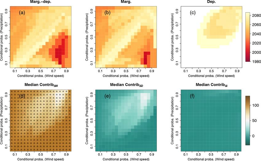
B. François and M. Vrac: Time of emergence of compound events                                                                             25

Figure 1. (a) Map of France with the regions of interest in boxes. Scatterplots of CNRM-CM6 (b) DJF compounding wind and precipitation
in Brittany and (c) minimal temperature in April and GDD values by the end of March over central France for the 1871–2100 period.
Parametric fitting for marginal and dependence over the 30-year sliding windows spanning the 1871–2100 period to bivariate points in orange.
For compounding wind and precipitation, these points correspond to high values of wind and precipitation data belonging to S90,90 CNRM-CM6 ,
i.e. simultaneously exceeding the individual 90th percentiles of the 1871–1900 reference period. Bivariate exceedance probabilities are then
computed for varying exceedance thresholds between the 5th and 95th percentile of wind speed and precipitation already belonging to
  CNRM-CM6 (for more details, see Sect. 4). The red area contains bivariate points exceeding the 80th percentiles of points already belonging
S90,90
    CNRM-CM6 . For growing-period frost, exceedance thresholds of interest for minimal temperature and GDD index are fixed to values of
to S90,90
0 and 200 ◦ C.day, respectively.

confidence intervals (i.e. out of the estimated natural vari-            3.2   Copula functions and exceedance probability
ability). The ToE is then defined as the central year of the
sliding window over which the probability starts to emerge.              In this study, we use copula modelling to compute CE proba-
As probabilities are estimated using copula modelling (see               bilities. We first consider two random variables X (e.g. max-
later in Sect. 3.2), 68 % and 95 % confidence intervals of the           imum wind speed) and Y (e.g. precipitation) for an arbitrary
baseline period’s probabilities are computed by coupling the             period. We denote their marginal (i.e. univariate) probabil-
parameter uncertainties of both the fitted marginal distribu-            ity density functions (pdfs) fX (x) and fY (y) and cumulative
tions and the fitted copula. Considering both 68 % and 95 %              marginal distribution functions (CDFs) FX (x) = P(X ≤ x)
confidence intervals allows us to evaluate, with different de-           and FY (y) = P(Y ≤ y). Sklar’s theorem (Sklar, 1959) states
grees of confidence, the changes of probability of compound-             that, H , the joint (i.e. bivariate) CDF can be written as:
ing events from the estimated natural variability. Details on
                                                                         HX,Y (x, y) = P(X ≤ x ∩ Y ≤ y) = C(FX (x), FY (y)),             (1)
the procedure to compute confidence intervals are given in
Appendix A.                                                              where C is a function called “copula”, corresponding to
                                                                         the joint distribution function of the uniformly distributed

https://doi.org/10.5194/nhess-23-21-2023                                              Nat. Hazards Earth Syst. Sci., 23, 21–44, 2023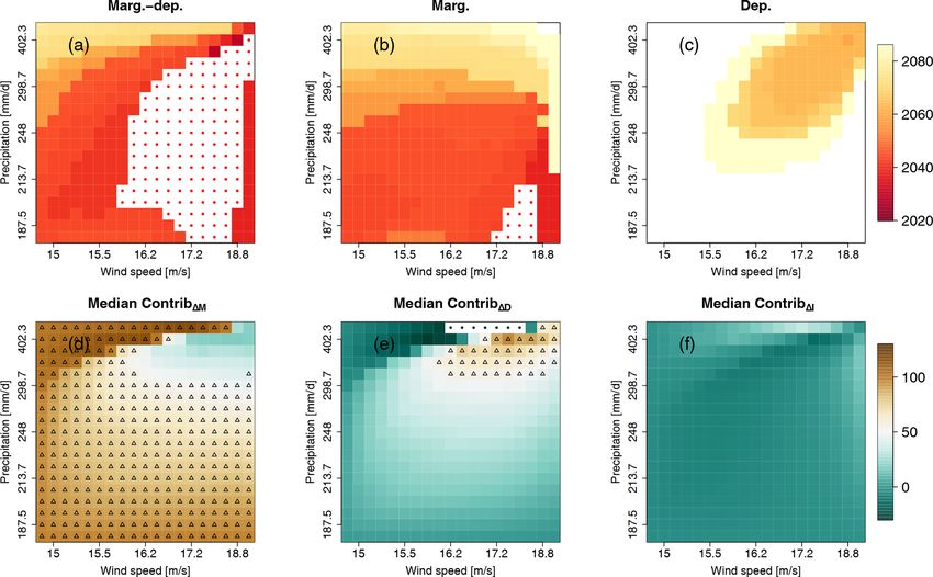
26                                                              B. François and M. Vrac: Time of emergence of compound events

variables FX (X) and FY (Y ). Under the assumption that the                 Then, do exceedance probability values change signifi-
marginal distributions FX and FY are continuous, Sklar’s                 cantly between reference and future periods? And if so, how
theorem states that the copula C is unique. This decompo-                much of this change is due to changing marginal properties,
sition of the multivariate distribution into marginal distri-            and how much is due to changing dependence structure? At-
butions and copula function allows us to model the depen-                tributing probability changes to changes of marginal and de-
dence among contributing variables independently of their                pendence properties has already been introduced by Bevac-
marginals. Therefore, using copulas makes it easy to iso-                qua et al. (2019) to analyse compound flooding from precip-
late the effects of marginal and dependence properties on the            itation and storm surge in Europe. However, to our knowl-
probability of multivariate hazards.                                     edge, assessing those changes relative to a reference natural
   Bivariate exceedance probability refers to the probability            variability in a ToE context has not been done yet. In or-
that both random variables exceed a certain value (“AND ap-              der to isolate the effects of these potentially changing sta-
proach”; Salvadori et al., 2016) and can be calculated rela-             tistical properties, we propose to calculate two additional ex-
tively easily using copulas. For example, for wind and pre-              ceedance probability values. The first one is the probability
cipitation CEs, it corresponds to probabilities of wind speed            pmfut ,dref , which assesses what the future probability would
and precipitation jointly exceeding established thresholds.              be if only the marginal properties change between the ref-
We denote pm,d the bivariate exceedance probability com-                 erence and future period (and thus keeping the dependence
puted with marginal (subscript m) and dependence (sub-                   properties from the reference period). pmfut ,dref is hence com-
script d) properties of (X, Y ). The probability pm,d (tX , tY )         puted as
that both X and Y jointly exceed some predefined thresh-
olds tX and tY is given by (Yue and Rasmussen, 2002; Shiau,              pmfut ,dref (tX , tY ) = 1 − FXfut (tX ) − FYfut (tY )
2003)                                                                                        + Cref (FXfut (tX ), FYfut (tY )).          (5)
pm,d (tX , tY ) = P(X ≥ tX ∩ Y ≥ tY )
                                                                         Inversely, the second additional probability pmref ,dfut is aimed
               = 1 − FX (tX ) − FY (tY )                                 at assessing what the future probability would be if only the
               + C(FX (tX ), FY (tY )).                           (2)    dependence properties change between the reference and fu-
                                                                         ture period (keeping the marginal properties from the refer-
Marginal and copula distributions in Eq. (2) are estimated us-           ence period), and is computed as
ing parametric fitting procedures. More details on the fitting
procedures for compound wind and precipitation extreme                   pmref ,dfut (tX , tY ) = 1 − FXref (tX ) − FYref (tY )
and growing-period frost events are given in Appendix B.
                                                                                             + Cfut (FXref (tX ), FYref (tY )).          (6)
3.3     Change in probabilities: contribution of the
                                                                         Illustrations of these four probabilities for artificial bivariate
        marginal and dependence properties
                                                                         distributions and changes between a reference and a future
Let us now consider the realisations (Xref , Yref ) and                  period are given in Fig. 2.
(Xfut , Yfut ) of the two random variables X and Y over the                 To assess how much marginal and dependence properties
reference period (i.e. 1871–1900 in the following), and over             contribute to exceedance probabilities change between refer-
another 30-year period (e.g. a future period such as 2071–               ence and future period, we use the four probabilities derived
2100). Using Eq. (2), the reference and future bivariate ex-             above to decompose the overall probability change. We first
ceedance probability pmref ,dref (tX , tY ) and pmfut ,dfut (tX , tY )   define 1P , the change of probability between the reference
for some predefined thresholds tX and tY are given by                    and future periods, as the difference between the two prob-
                                                                         abilities: 1P = pmfut ,dfut − pmref ,dref . By computing pmfut ,dref
pmref ,dref (tX , tY ) = 1 − FXref (tX ) − FYref (tY )                   and pmref ,dfut , one can decompose the change of probability
                    + Cref (FXref (tX ), FYref (tY )),            (3)    1P into a sum of three terms that can yield statistical inter-
                                                                         pretations:
pmfut ,dfut (tX , tY ) = 1 − FXfut (tX ) − FYfut (tY )
                    + Cfut (FXfut (tX ), FYfut (tY )).            (4)    1P = 1M + 1D + 1I.                                              (7)
As modelled here with Eqs. (3) and (4), pmfut ,dfut and mfut ,dfut       The first term 1M accounts for the difference of probability
can differ due to                                                        between the reference and future periods due to a change of
     – changes in the marginal properties of X and Y , i.e.              marginal properties only and is hence called the “marginal”
       changes between FXref and FXfut , as well as between              term:
       FYref and FYfut ,
                                                                         1M = pmfut ,dref − pmref ,dref
     – and changes in the dependence structure (i.e. in the cop-
       ulas) between X and Y , i.e. changes between Cref and             Similarly, the second term 1D assesses the difference of
       Cfut .                                                            probability between the reference and future periods due to

Nat. Hazards Earth Syst. Sci., 23, 21–44, 2023                                                https://doi.org/10.5194/nhess-23-21-2023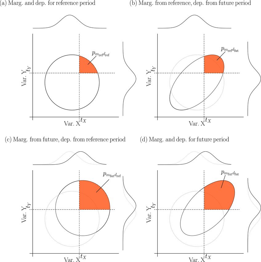
B. François and M. Vrac: Time of emergence of compound events                                                                                  27

Figure 2. Illustration of the influence of marginal and dependence properties on bivariate exceedance probabilities for an artificial distribution
of two contributing variables X and Y during (a) the reference period and (d) a future period with a shift in means and an increase in
dependence between the variables. The distribution of the two contributing variables (b) with marginal properties from the reference period
and dependence structure from the future period, and (c) with marginal properties from the future period and dependence structure from the
reference period. Orange areas show bivariate exceedance probabilities for the thresholds (tX , tY ) of the two contributing variables.

a change of dependence properties only and is hence called                 the effects of the changes of dependence properties and the
the “dependence” term:                                                     effects of the changes of interaction on the overall change of
                                                                           probability value 1P . By taking advantage of this decompo-
1D = pmref ,dfut − pmref ,dref                                             sition, we propose to quantify the contribution (in %) of the
                                                                           different terms 1M, 1D and 1I to the change of probabil-
As simultaneous changes of marginal and dependence prop-
                                                                           ity 1P . For example, the contribution of the changes of the
erties between the reference and future period can affect the
                                                                           marginal properties can be quantified as
exceedance probability in a highly non-linear fashion (as can
be seen in Fig. 2), 1P cannot be simply expressed as the                                    1M         pmfut ,dref − pmref ,dref
                                                                           Contrib1M =         ×100, =                           ×100. (8)
sum of the differences 1M and 1D. Thus, a residual term                                     1P         pmfut ,dfut − pmref ,dref
1I , called the “interaction” term, is introduced to assess the
                                                                           A value of 50 % for Contrib1M would indicate that the
part of the probability change that is due to the simultaneous
                                                                           change of marginal properties is responsible for 50 % of the
change of marginal and dependence properties and that can-
                                                                           global change of probability 1P between the reference and
not be explained by the changes of these statistical properties
                                                                           future periods. The contributions of 1D (or 1I ) can be cal-
separately:
                                                                           culated the same way by simply replacing 1M in Eq. (8)
1I = pmfut ,dfut − pmfut ,dref − pmref ,dfut + pmref ,dref .               by 1D (or 1I ). The sum of the three contributions adds up
                                                                           to 100 %, by construction. Please note that, for illustration,
The decomposition of 1P into these three terms allows us                   changes of probability 1P , 1M and 1D are here consid-
to isolate the effects of the changes of marginal properties,              ered as differences of probabilities. One could also consider

https://doi.org/10.5194/nhess-23-21-2023                                                 Nat. Hazards Earth Syst. Sci., 23, 21–44, 2023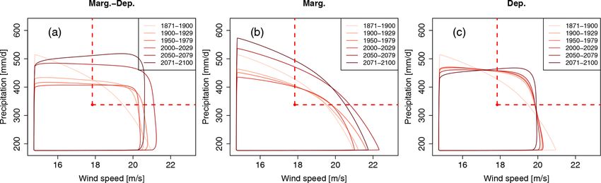
28                                                                     B. François and M. Vrac: Time of emergence of compound events

analysing other metrics such as relative differences (“r. diff”)               4     Results for compounding wind and precipitation
by dividing each of the terms in Eq. (7) by pmref ,dref :                            extremes

             pmfut ,dfut − pmref ,dref                                         In this section, results are presented for compound wind and
1P r. diff =                            ,
                     pmref ,dref                                               precipitation extremes during winter in Brittany. Please note
              pmfut ,dref − pmref ,dref                                        that, for this section as well as for the rest of the study, the pe-
1M r. diff =                             ,
                      pmref ,dref                                              riod 1871–1900 is considered as the baseline period for nat-
             pmref ,dfut − pmref ,dref                                         ural variability to evaluate ToE and contributions. To focus
1D r. diff =                            ,                                      on wind and precipitation extremes, we applied our method-
                     pmref ,dref
                                                                               ology to points of high values. For each model, we selected
             pmfut ,dfut − pmfut ,dref − pmref ,dfut + pmref ,dref
1I r. diff =                                                       .           points where, concurrently, wind and precipitation values ex-
                                  pmref ,dref                                  ceed the individual 90th percentiles (denoted xsel and ysel ,
In addition, bivariate fraction of attributable risk (“FAR”,                   respectively) of the 1871–1900 reference period. In the fol-
                                                                                                      i
                                                                               lowing, we denote S90,90    the ensemble of the selected points
e.g. Stott et al., 2016; Chiang et al., 2021; Zscheischler and
Lehner, 2021) can also be computed by dividing each of the                     of high values for a model i. For illustrative purpose, the en-
                                                                                          CNRM-CM6 for the CNRM-CM6 model is shown in
                                                                               semble S90,90
terms by pmfut ,dfut :
                                                                               orange in Fig 1b. We first illustrate our method with a single
         pmfut ,dfut − pmref ,dref                                             climate model (CNRM-CM6). Then, results obtained for the
1P FAR =                            ,                                          Indiv-Ensemble version are presented.
                 pmfut ,dfut
          pmfut ,dref − pmref ,dref
1M FAR =                             ,                                         4.1    Results for an individual model and a single
                  pmfut ,dfut
                                                                                      exceedance threshold: CNRM-CM6
         pmref ,dfut − pmref ,dref
1D FAR =                            ,
                 pmfut ,dfut                                                   To illustrate our methodology, we first explain the results ob-
         pmfut ,dfut − pmfut ,dref − pmref ,dfut + pmref ,dref                 tained for compound wind and precipitation extremes and a
1I FAR =                                                       .
                              pmfut ,dfut                                      single bivariate exceedance threshold before extending the
                                                                               results to several bivariate thresholds. We evaluate the prob-
However, by construction, results for contributions, either for                abilities of exceeding the 80th percentiles of the bivariate
relative differences or bivariate FAR, would be identical to                                            CNRM-CM6 . The 80th percentiles for
                                                                               points belonging to S90,90
those obtained for differences.
                                                                               wind and precipitation correspond to x80|sel ≈ 17.8 m s−1
   The methodology described above to assess ToE of CE
                                                                               and y80|sel ≈ 338 mm d−1 , respectively.
probabilities and marginal and dependence contributions to
                                                                                  Before computing any probability, Fig. 4 gives an initial
these changes is applied to the 13 CMIP6 models by consid-
                                                                               overview of the fitted bivariate distributions of compound
ering successively all 30-year sliding windows spanning the
                                                                               wind and precipitation extremes in our study. It displays the
period 1871–2100. The methodology is applied to each cli-
                                                                               evolution of the bivariate distributions over a selection of
mate model individually (“Indiv-Ensemble” version). In par-
                                                                               sliding windows due to changing marginal and dependence
ticular for contributions and ToE, multi-model median esti-
                                                                               properties (“Marg.-dep.”, Fig. 4a), changing marginal prop-
mates are derived to summarise the information given by all
                                                                               erties only (“Marg.”, Fig. 4b) and changing dependence only
the models. The Indiv-Ensemble version makes it possible to
                                                                               (“Dep.”, Fig. 4c). Plotting these bivariate distributions al-
analyse the modelling of hazards separately and to assess the
                                                                               ready indicates the changes in probability of wind and pre-
uncertainty in ToE arising from the inter-model differences.
                                                                               cipitation extremes, and the potential influences of marginal
We also applied the methodology in the “Full-Ensemble”
                                                                               and dependence properties on these changes. Indeed, at first
version, which consists of pooling the contributing variables
                                                                               sight in Fig. 4a, the area of bivariate distributions where wind
of the 13 climate models together to derive unique ToE esti-
                                                                               speed and precipitation jointly exceed x80|sel and y80|sel ap-
mates and contribution values accounting for the global un-
                                                                               pears to increase for future periods, suggesting that such bi-
certainty in climate modelling. However, the details of the
                                                                               variate events are more likely to occur according to CNRM-
“Full-Ensemble” version and its results are not discussed in
                                                                               CM6 projections. But is this change of probability signifi-
the main article but are given in Sects. S1–S5 in the Supple-
                                                                               cant? And is this change due to changes in marginal proper-
ment. A summary of the successive steps of our methodology
                                                                               ties or in dependence properties or in both? By keeping the
for the Indiv-Ensemble version is provided in the form of a
                                                                               dependence properties of the reference period and consider-
flowchart in Fig. 3.
                                                                               ing changing marginal properties only (Fig. 4b), an increase
                                                                               of exceedance probability seems to be observed, although
                                                                               less pronounced. Similar observations can be made by keep-
                                                                               ing the marginal properties of the reference period and con-
                                                                               sidering changing dependence properties only (Fig. 4c). If

Nat. Hazards Earth Syst. Sci., 23, 21–44, 2023                                                    https://doi.org/10.5194/nhess-23-21-2023
B. François and M. Vrac: Time of emergence of compound events 29 Figure 3. Flowchart for the computations of time of emergence and contributions for the Indiv-Ensemble version. both marginal and dependence changes seem to have an im- the 68 % confidence level, in 2073 (2058–2087) and 2063 portance in the increase of probability, it is important to (2048–2077), respectively. If contributions of the statistical quantify how much these statistical properties contribute to properties to ToE in itself are not computed here, one can the change of the overall probability as well as their respec- get an idea of the importance of the statistical properties tive influence on the ToE of probabilities of compounding in ToE: at the 68 % confidence level, ignoring the depen- wind and precipitation extremes. dence change would induce a ToE 2073 − 2009 = 64 years Time series of exceedance probabilities over all sliding later. Similarly, ignoring marginal changes would induce a windows for the bivariate threshold (x80|sel , y80|sel ) are pre- ToE 2063 − 2009 = 54 years later. It thus indicates that both sented in Fig. 5 by considering changes of marginal and de- marginal and dependence properties have a non-negligible pendence properties together (Fig. 5a) and separately (Fig. 5b effect on ToE. and c). The 68 % and 95 % confidence intervals resulting The evolution of the bivariate FAR 1P FAR with respect to from marginal and copula uncertainties are also displayed the reference period over sliding windows, as well as its de- for each probability. All three time series present an increase composition in terms of “marginal” (1M FAR ), “dependence” with time, which is consistent with the visual analysis made (1D FAR ) and “interaction” (1I FAR ) terms, is displayed in in Fig. 4. Probability increase is less pronounced when future Fig. 5d. As explained in Sect. 3, for each sliding window, marginal (Fig. 5b) and future dependence properties (Fig. 5c) the sum of 1M FAR , 1D FAR and 1I FAR is by construction are considered separately. It illustrates that the effects of equal to 1P FAR . The decomposition highlights that the in- these changing statistical properties combine on exceedance fluences of the marginal and of the dependence properties probabilities. Yet, all three probability signals permanently on bivariate FAR can vary with time. Also, the combination go out of the reference natural variability confidence inter- of individual effects of marginal and dependence changes on vals, suggesting that an emergence of probability occurs: for the overall probability changes is again illustrated: for ex- probabilities computed with future marginal and dependence ample, by 2100, considering both future marginal and de- properties (Fig. 5a), the ToE is detected in 2009 (1994–2023) pendence changes leads to a value of FAR 1P FAR twice and 2072 (2057–2086) for 68 % and 95 % confidence lev- as high as those of 1M FAR and 1D FAR , respectively. Con- els, respectively. Concerning probabilities influenced by fu- cerning the interaction term, its associated bivariate FAR is ture marginal changes and future dependence changes sep- negligible, highlighting that most of the changes can be ex- arately (Fig. 5b and c), probability signals emerge later at plained by the changing marginal and dependence properties https://doi.org/10.5194/nhess-23-21-2023 Nat. Hazards Earth Syst. Sci., 23, 21–44, 2023
30                                                                B. François and M. Vrac: Time of emergence of compound events

Figure 4. Change of winter (December to February) bivariate wind and precipitation extremes distributions in Brittany based on CNRM-
CM6 simulations due to (a) future marginal and dependence changes (“Marg.-dep.”), (b) future marginal changes while keeping dependence
properties of the reference period (“Marg.”) and (c) dependence changes while keeping marginal properties of the reference period (“Dep.”).
For the bivariate distributions, contour lines encompassing 90 % of all data points are shown. A selection of six 30-year sliding windows are
presented using a colour gradient from light (1871–1900) to dark (2071–2100). The dashed red lines characterise the bivariate exceedance
thresholds defined here as the 80th quantile of each variable.

Figure 5. (a–c) Probability changes and time of emergence of compound wind and precipitation extremes P X > x80|sel ∩ Y >
                    CNRM-CM6

y80|sel |(X, Y ) ∈ S90,90         based on CNRM-CM6 simulations due to changes of (a) both marginal and dependence properties,
(b) marginal properties only, and (c) dependence properties only. The shaded bands indicate 68 % and 95 % confidence intervals of the
probabilities. Evolution of (d) the bivariate fraction of attributable risk (FAR), (e) relative difference of probabilities with respect to the refer-
ence period (1871–1900) and (f) contribution of the marginal, dependence and interaction terms to probability values. Median contributions
computed over all sliding windows are displayed with dashed lines. Asterisks indicate values lying outside the plotted range. Not applicable
(n/a) is indicated when no time of emergence is detected.

Nat. Hazards Earth Syst. Sci., 23, 21–44, 2023                                                    https://doi.org/10.5194/nhess-23-21-2023
B. François and M. Vrac: Time of emergence of compound events 31
separately. Results for relative differences are displayed in than when considering only marginal changes (Fig. 6b). Con-
Fig. 5e, and the same conclusions can be drawn. Figure 5f cerning the median contributions over all sliding windows
shows the evolution of the contributions from the marginal, of the marginal (Fig. 6d), dependence (Fig. 6e) and interac-
dependence and interaction terms to probability values over tions terms (Fig. 6f), results vary according to the exceedance
sliding windows. By computing the median of contributions thresholds considered. Whereas for a large proportion of the
over all sliding windows, we can see that both changes in the exceedance thresholds, changes in marginal properties con-
marginal and in the dependence properties contribute greatly tribute strongly to probability changes (Fig. 6d), changes in
to probability changes (≈ 50 %) in the CNRM-CM6 simula- dependence properties contribute predominantly to probabil-
tions, with a slightly more important contribution from de- ity changes of very high wind and precipitation extremes
pendence properties (dashed lines in Fig. 5f). One may note (Fig. 6e). Regarding the “interaction” term, its contributions
a symmetry between the contribution values of the marginal are close to 0, indicating little influence on the probability
and the dependence terms over sliding windows. This can changes.
be explained by the way contribution values are computed.
Indeed, as the sum of the three contributions adds up to 4.3 Results for the Indiv-Ensemble version and a single
100 %, by construction, and the fact that the contribution exceedance threshold
from the interaction term is close to 0, contribution values
of the marginal and the dependence terms covary symmetri- We now present the results obtained for ToE and contribu-
cally around 50 %. tions for the Indiv-Ensemble version for a single exceedance
threshold. The methodology, previously illustrated with the
4.2 Results for CNRM-CM6 and several exceedance CNRM-CM6 simulations, is now applied to each of the 13
thresholds models. Among the 13 models of the ensemble, only one
model (INMCM-5.0) had more than 5 % of goodness-of-fit
The results for ToE and contributions have so far been pre- tests over all sliding windows, thus rejecting the hypothesis
sented for the probability of events exceeding the 80th per- that the copula is a good fit, and hence was excluded from
CNRM-CM6 . In or-
centiles of selected points belonging to S90,90 the analysis (see Appendix B for further details).
der to have a broader analysis of exceedance probabilities We first present the results obtained for probabilities of ex-
of compound wind and precipitation extremes, we repeat the ceeding the 80th percentiles of selected points of high values
methodology for all pairs of exceedance thresholds between of wind and precipitation for the 1871–1900 reference pe-
the 5th and 95th percentiles (with steps of 5 percentiles) of riod. Figure 7 presents the results obtained. Probability time
CNRM-CM6 . Figure 6 displays
selected points belonging to S90,90 series obtained for the 12 models when considering changes
the results obtained for the CNRM-CM6 ToE at the 68 % of marginal and dependence properties(Fig. 7a), marginal
confidence level, by considering marginal and dependence properties (Fig. 7b) and dependence properties (Fig. 7c) are
changes (Fig. 6a), marginal changes only (Fig. 6b) and de- displayed, as well as ToE at the 68 % confidence level for the
pendence changes only (Fig. 6c). Moreover, for each bivari- individual models and their multi-model median estimate.
ate exceedance threshold, median contributions (over all slid- When considering future changes of both marginal and de-
ing windows) of marginal (Fig. 6d), dependence (Fig. 6e) pendence properties (Fig. 7a), half of the models (6/12) de-
and interaction terms (Fig. 6f) are displayed. Results for tect a ToE at the 68 % confidence level. When found, a rel-
ToE obtained at the 95 % confidence level are displayed in atively important variability of ToE across climate models
Fig. S2 and differences of ToE are displayed in Fig. S3. When is obtained (varying between 2009 (1994–2023) and 2083
varying the exceedance thresholds, different ToE results are (2068–2097), Fig. 7a). These different results – i.e. either a
obtained, depending on whether marginal and dependence ToE is detected or not, and the important variability of the
changes are considered (Fig. 6a–c). ToE is found for most of year of emergence when found – indicate discrepancies in
the exceedance thresholds when considering both marginal the statistical properties of compound wind and precipita-
and dependence changes (Fig. 6a) or marginal changes only tion extremes between climate models. For marginal changes
(Fig. 6b). It is, however, not the case for dependence changes (Fig. 7b), seven models out of 12 detect a ToE, within a
only (Fig. 6c), for which only specific pairs of exceedance smaller range of values. It suggests a slightly better agree-
thresholds can find ToE. Interestingly, these pairs correspond ment of marginal changes for future periods between mod-
to very high compound wind and precipitation extremes. els when ToE is defined. Moreover, models that show emer-
This indicates that dependence change plays an important gence when considering marginal changes only are not nec-
role for the probability of such high extreme events. The essarily those that show emergence when considering both
importance of dependence properties can also be assessed future marginal and dependence changes. Indeed, two out
visually by comparing Figs. 6a and b. Indeed, for approxi- of the seven models emerging with marginal changes are
mately the same pairs of exceedance thresholds as those al- not those from the six emerging when marginal and depen-
ready identified in Fig. 6c, earlier ToEs are obtained when dence changes are taken into account (not shown). Hence,
considering both marginal and dependence changes (Fig. 6a) marginal changes alone are not always sufficient to make the
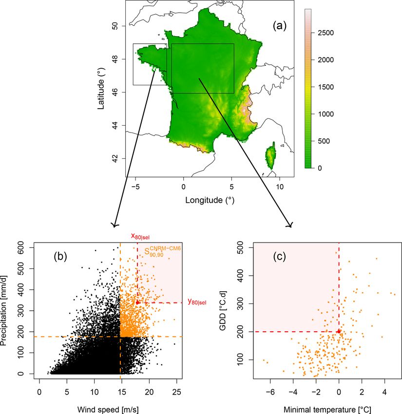
https://doi.org/10.5194/nhess-23-21-2023 Nat. Hazards Earth Syst. Sci., 23, 21–44, 202332 B. François and M. Vrac: Time of emergence of compound events Figure 6. CNRM-CM6 (a–c) time of emergence (at 68 % confidence level) for compound wind and precipitation extremes due to changes of (a) both marginal and dependence properties, (b) marginal properties only, and (c) dependence properties only. White cells indicate that no time of emergence is detected, while white cells with red points indicate time of emergence values before 2020. (d–f) Matrices of median contributions of the (d) marginal, (e) dependence and (f) interaction terms. Results are presented for varying exceedance thresholds between the 5th and 95th percentile of compound wind and precipitation extremes data. Upper triangles show where the contribution is ≥ 50 %. probability signal emerge. Concerning dependence changes highlights again that the influences of the marginal and of the (Fig. 7c), two models out of 12 detect a ToE, indicating that dependence properties on bivariate FAR, relative differences dependence property changes for these two models influence and contributions can vary with time. greatly the exceedance probabilities by 2100. However, it Figure 7g displays the median contributions over all slid- also suggests that, for most of the models, the influence of ing windows for the 12 climate models separately, as well the changes in dependence properties on exceedance proba- as for the Indiv-Ensemble version, i.e. by computing the bilities is too small to make the probability signals go out of median contribution of the models. Figure 7g shows that, the reference confidence interval by 2100. These results on depending on the model, different results are obtained for the stationarity of dependence structures complement those the contributions to probability changes. Indeed, while some of Vrac et al. (2022b), where the ability of CMIP6 models to models present balanced contributions, i.e. marginal and de- capture and represent significant changes in inter-variable de- pendence terms contributing to ≈ 50 % each to probability pendencies is questioned. ToE results at the 95 % confidence changes (e.g. CMCC-ESM2, CNRM-CM6-1 and CNRM- level are displayed in Fig. S5 and are summarised using box- CM6-1-HR), other models show very unbalanced contribu- plots in Fig. S7. tions, with one statistical property mainly driving the proba- The evolution of bivariate FAR, relative differences and bility changes. For example, the dependence term contributes contributions time series with respect to the reference pe- predominantly (≥ 65 %) to probability changes for the mod- riod, as well as their decomposition in terms of marginal, els CanESM5, FGOALS-g3 and INM-CM-4-8, while the dependence and interaction terms, is displayed in Fig. 7d– marginal term contributes the most for EC-Earth3, GFDL- f, respectively. For reasons of brevity, the median of the 12 CM4, IPSL-CM61-LR, MIROC6, MPI-ESM1-2-LR and models’ FAR, relative differences and contributions com- MRI-ESM2-0. Results for the Indiv-Ensemble version indi- puted at each sliding window is plotted. The decomposition cate the contribution to probability changes of ≈ 60 % from Nat. Hazards Earth Syst. Sci., 23, 21–44, 2023 https://doi.org/10.5194/nhess-23-21-2023
B. François and M. Vrac: Time of emergence of compound events                                                                             33

Figure 7. (a–c) Same as Fig. 5a–c but for the 12 individual CMIP6 models of the ensemble. Individual time of emergence is displayed
when defined (vertical light red lines), as well as the corresponding median time of emergence (vertical red line). For information purposes,
multi-model mean exceedance probability time series are also plotted (dotted black lines). (d–f) Same as Fig. 5d–f but for the Indiv-Ensemble
version. Bivariate FAR, relative differences and contributions time series are computed by considering for each sliding window the median
of the models’ FAR, relative differences and contributions, respectively. (g) Median contribution of the marginal, dependence and interaction
terms to overall probability changes for the 12 models and for the Indiv-Ensemble version.

https://doi.org/10.5194/nhess-23-21-2023                                              Nat. Hazards Earth Syst. Sci., 23, 21–44, 2023
34                                                         B. François and M. Vrac: Time of emergence of compound events

changes in marginal properties and ≈ 40 % from changes in          than 50 %, but specific pairs of exceedance thresholds high-
dependence properties. Concerning the interaction term, as         light again the varying importance of dependence properties
obtained previously in Sect. 4.1, its contribution is close to 0   in exceedance probability changes: the median contribution
for each model individually.                                       of dependence properties is high for the probability changes
                                                                   of events exceeding high wind speed and high precipitation
4.4   Results for the Indiv-Ensemble version and several           values. Concerning the interaction term (Fig. 8f), contribu-
      exceedance thresholds                                        tion values are equal to 0, highlighting again the negligi-
                                                                   ble role of this term in probability changes. ToE results at
As previously done in Sect. 4.2, we now compute ToE for            the 95 % confidence level as well as the number of models
all combinations of exceedance thresholds between the 5th          emerging at the 95 % confidence level and interquartile val-
and 95th percentiles in Fig. 8. Note that, here, exceedance        ues are shown in Figs. S11 and S12, respectively.
thresholds are now expressed in terms of percentiles to en-
able a comparison of results. Figure 8a shows multi-model
medians of ToE values induced by both marginal and depen-          5     Results for growing-period frost events
dence changes, i.e. results obtained for the Indiv-Ensemble
                                                                   We now apply our methodology to analyse a second type of
version. A median value of ToE is obtained for any consid-
                                                                   CE: growing-period frost. Contrary to compound wind and
ered bivariate threshold, indicating that, for each exceedance
                                                                   precipitation extremes, for which we were interested in ex-
threshold, at least one model presents an emergence. How-
                                                                   ceedance probabilities (i.e. both contributing variables ex-
ever, median ToE values show a variability depending on
                                                                   ceedance thresholds), we are interested here in the proba-
the bivariate exceedance thresholds. Note that the number
                                                                   bility of growing-period frost, i.e. the probability of having
of models presenting a ToE can also vary from one bivari-
                                                                   a GDD value exceeding a threshold of 200 (GDD ≥ 200) by
ate threshold to another. For each exceedance threshold, the
                                                                   the end of March – and hence characterising bud burst condi-
number of models emerging at the 68 % confidence level, as
                                                                   tions – and having a frost in April, i.e. having T ≤ 0. Hence,
well as interquartile values, are shown in Fig. S8. In partic-
                                                                   we applied our methodology described in Sect. 3 to bivari-
ular, Fig. S8a indicates that all of the 12 models present a
                                                                   ate points of GDD and minimal temperature data (one pair
ToE for the probability of events exceeding very high pre-
                                                                   by year) by adapting Eq. (2) to compute the probabilities of
cipitation and relatively low wind speed values (upper-left
                                                                   interest. For example, for the probability of growing-period
corner of the subplot). It suggests that all models agree on a
                                                                   frost in the reference period, it is computed as follows (Yue
change of the probability of occurrence of such events. This
                                                                   and Rasmussen, 2002):
large consensus between models is not reached for events ex-
ceeding relatively low precipitation and very high wind speed      pm,d (0, 200) = P(T ≤ 0 ∩ GDD ≥ 200)
values. Therefore, while all models simulate a significant in-
                                                                                 = FT (0) − C(FT (0), FGDD (200)).             (9)
crease of extreme precipitation events, this is not necessarily
the case for extreme wind speed events. Results obtained for       Although the main results are presented for a threshold
ToE induced by marginal properties only (Figs. 8b and S8b)         of 200 ◦ C.day, additional results for thresholds of 150 and
are quite similar, although still indicating small differences     250 ◦ C.day are displayed in the Supplement to assess risks
with those obtained by considering marginal and dependence         of growing-period frost for earlier and later bud burst plants.
changes. Indeed, small differences of ToE can be observed,
in particular for the upper-right area corresponding to very       5.1    Indiv-Ensemble results
high wind speed and precipitation extremes. As observed in
Sect. 4.1, this area corresponds to the area where changes         We now present the results for the growing-period frost.
in dependence properties lead to emerging exceedance prob-         As previously done, only one model (CMCC-ESM2) is ex-
ability from the reference period (Fig. 8c), suggesting their      cluded from the ensemble since it presents more than 5 % of
importance for the probability changes of such events. This        goodness-of-fit tests, thus rejecting the hypothesis that fitted
result, however, should not be overstated, as only ≈ 2 models      copulas are a good fit (see Appendix B for further details).
show dependence changes large enough to lead to the emer-             Figure 9 presents the results obtained for growing-period
gence of probability (Fig. S8c).                                   frost events. Results for 150 and 250 ◦ C.day GDD thresholds
   Median contribution of marginal, dependence and interac-        are presented in the Supplement in Figs. S15 and S16, respec-
tions terms is displayed in Fig. 8d–f, respectively. The re-       tively. By considering climate models separately, a ToE at
sults obtained previously concerning the importance of the         the 68 % confidence level is detected for 11 out of 12 models
marginal properties in probability changes are confirmed           when changes in marginal properties are taken into account
here: for all exceedance thresholds, changes in marginal           (Fig. 9a and b). Although a large majority of models agree
properties contribute to more than 50 % of probability             by simulating a significant change of growing-period frost
changes (Fig. 8d). Concerning the contribution of depen-           probability with respect to the reference period, ToE val-
dence changes (Fig. 8e), the median values obtained are less       ues are quite scattered, indicating differences in simulations

Nat. Hazards Earth Syst. Sci., 23, 21–44, 2023                                       https://doi.org/10.5194/nhess-23-21-2023
You can also read