A global algorithm for identifying changing streamflow regimes: application to Canadian natural streams (1966-2010)
←
→
Page content transcription
If your browser does not render page correctly, please read the page content below
Hydrol. Earth Syst. Sci., 25, 5193–5217, 2021
https://doi.org/10.5194/hess-25-5193-2021
© Author(s) 2021. This work is distributed under
the Creative Commons Attribution 4.0 License.

A global algorithm for identifying changing streamflow regimes:
application to Canadian natural streams (1966–2010)
Masoud Zaerpour1 , Shadi Hatami1 , Javad Sadri2 , and Ali Nazemi1
1 Department  of Building, Civil and Environmental Engineering, Concordia University, Montreal, Quebec, Canada
2 Oppimi   Group, Montréal, Quebec, Canada

Correspondence: Masoud Zaerpour (masoud.zaerpour@concordia.ca) and Ali Nazemi (ali.nazemi@concordia.ca)

Received: 1 July 2020 – Discussion started: 31 August 2020
Revised: 1 July 2021 – Accepted: 18 August 2021 – Published: 24 September 2021

Abstract. Climate change affects natural streamflow regimes        impacts of climate change on streamflow regimes in cold re-
globally. To assess alterations in streamflow regimes, typi-       gions.
cally temporal variations in one or a few streamflow charac-
teristics are taken into account. This approach, however, can-
not see simultaneous changes in multiple streamflow char-
acteristics, does not utilize all the available information con-   1   Introduction
tained in a streamflow hydrograph, and cannot describe how
and to what extent streamflow regimes evolve from one to           Natural characteristics of streamflow are critical to ecosys-
another. To address these gaps, we conceptualize streamflow        tem livelihood and human settlements around river systems
regimes as intersecting spectrums that are formed by multi-        (Poff et al., 2010; Nazemi and Wheater, 2014; Hassanzadeh
ple streamflow characteristics. Accordingly, the changes in        et al., 2017). Historically, humans have considered the sea-
a streamflow regime should be diagnosed through gradual,           sonality, variability, and magnitude of natural streamflow as
yet continuous changes in an ensemble of streamflow char-          key factors for determining potentials for socio-economic
acteristics. To incorporate these key considerations, we pro-      developments (Knouft and Ficklin, 2017). Streamflow char-
pose a generic algorithm to first classify streams into a finite   acteristics are diverse and can contain different informa-
set of intersecting fuzzy clusters. Accordingly, by analyzing      tion. While some streamflow characteristics determine po-
how the degrees of membership to each cluster change in a          tentials for agriculture and energy production (Hamududu
given stream, we quantify shifts from one regime to another.       and Killingtveit, 2012; Amir Jabbari and Nazemi, 2019;
We apply this approach to the data, obtained from 105 nat-         Nazemi et al., 2020), some others act as proxies for the con-
ural Canadian streams, during the period of 1966 to 2010.          sequences of devastating disasters such as floods or droughts
We show that natural streamflow in Canada can be catego-           (Arheimer and Lindström, 2015; Burn and Whitfield, 2016;
rized into six regime types, with clear hydrological and geo-      Zandmoghaddam et al., 2019).
graphical distinctions. Analyses of trends in membership val-         A set of streamflow characteristics, collectively defin-
ues show that alterations in natural streamflow regimes vary       ing the overall flow behaviour in a river reach, is called
among different regions. Having said that, we show that in         the streamflow regime (Poff et al., 1997). Traditionally,
more than 80 % of considered streams, there is a dominant          streamflow regimes have been considered stationary in time
regime shift that can be attributed to simultaneous changes        (Milly et al., 2008). However, the looming effects of cli-
in streamflow characteristics, some of which have remained         mate change along with human interventions through land
previously unknown. Our study not only introduces a new            and water management have raised fundamental questions
globally relevant algorithm for identifying changing stream-       regarding the stationarity of streamflow regimes during the
flow regimes but also provides a fresh look at streamflow al-      current “Anthropocene” (Arnell and Gosling, 2013; Nazemi
terations in Canada, highlighting complex and multifaceted         and Wheater, 2015a, b). Even in undisturbed streams, recent
                                                                   literature is full of evidence indicating major alterations in-

Published by Copernicus Publications on behalf of the European Geosciences Union.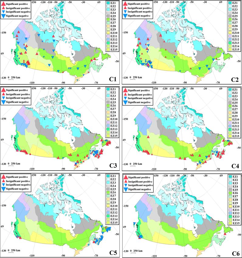
5194                                   M. Zaerpour et al.: A global algorithm for identifying changing streamflow regimes

duced by heightened climate variability and change (Barnett         2019), and changes in streamflow characteristics are signifi-
et al., 2005; Stahl et al., 2010; Rood et al., 2016; Hodgkins       cant in time and space (e.g., Buttle et al., 2016; O’Neil et al.,
et al., 2017; Dierauer et al., 2018). As a result, assessing how    2017; Dierauer et al., 2020). By considering more than 100
streamflow regimes are changing as a result of alterations in       natural streams, we provide – for the first time – a homo-
natural and anthropogenic drivers is currently one of the im-       geneous, pan-Canadian view on recent alterations in natural
minent questions in the field of hydrology.                         streamflow regimes. The remainder of this paper is as the fol-
   Despite the extensive body of knowledge already gathered         lowing: sect. 2 describes our three-step methodology related
around assessing the effects of climate change on altering          to (i) clustering regime types, (ii) detecting regime changes,
streamflow regimes, there is still room for methodological          and (iii) attributing regime changes to alterations in stream-
developments. Most importantly, among many potential flow           flow characteristics. Section 3 introduces our case study and
characteristics that can constitute and describe a streamflow       the data. The results and discussions are presented in Sects. 4
regime, often only a few are taken into account (Whitfield          and 5. Finally, Sect. 6 concludes our work and provides some
and Cannon, 2000; Hall et al., 2014; Vormoor et al., 2015).         further remarks.
This is a limitation because climate change impacts are often
manifested in the entire streamflow hydrograph and not only
around a unique set of streamflow characteristics (Olden and
Poff, 2003). This is particularly the case in cold regions as       2     Methodology
at the watershed scale, multiple processes contribute to the
streamflow generation, each behaving differently in response        2.1    Rationale and proposed algorithm
to climate variability and change (Whitfield and Pomeroy,
2016). As a result, alterations in streamflow regimes are not       From both conceptual and computational perspectives, quan-
only significant (e.g., Déry and Wood, 2005; MacDonald et           tifying changes in streamflow regimes is not a trivial task
al., 2018; Islam et al., 2019; Champagne et al., 2020), but         due to the relativity in the definition of streamflow regime
they are also complex due to compound impacts of changes            and how a change can be identified. On the one hand, the
in temperature, shifts in forms and magnitude of precipita-         flow regime at a given stream is defined by a large number
tion, and alterations in snow and ice accumulation and melt         of streamflow characteristics, some of which have conflict-
(DeBeer et al., 2016; Hatami et al., 2018; Rottler et al., 2020).   ing trends in time and space. On the other hand, the flow
At this stage of development, it is not yet possible to sys-        regime is often identified based on similarity/dissimilarity
tematically quantify streamflow regimes and their alterations       of characteristics in a set of benchmarking streams with
to one another using a large set of simultaneously changing         known regimes. Accordingly, regime shifts are not only de-
streamflow characteristics (Burn et al., 2016; Burn and Whit-       fined based on alterations in streamflow characteristics rela-
field, 2018).                                                       tive to the past but also with respect to relative changes as
   Here, we propose a new methodology to address this chal-         regards other streams with known regime types. This cre-
lenge. First, by considering more streamflow characteristics,       ates a complex mathematical problem due to the “curse of
the distinctions between regime types and their alterations         dimensionality” (see, for example, Trunk, 1979), meaning
become more fuzzy and relative. Accordingly, in line with           that the complexity of the problem increases exponentially
some recent suggestions in the literature (see, for example,        by increasing the number of streams and/or streamflow char-
Ternynck et al., 2016; Burn and Whitfield, 2017; Knoben             acteristics with which the streamflow regime is defined. To
et al., 2018; Brunner et al., 2018, 2019; Aksamit and Whit-         solve this problem, the general tendency in the literature is
field, 2019; Jehn et al., 2020), we conceptualize streamflow        to reduce the dimensionality of the problem through the use
regimes as continuous spectrums rather than distinct states.        of methodologies, such as multidimensional scaling, empir-
This conceptualization requires a methodology that can for-         ical orthogonal functions, and principal component analy-
mally deal with subjectivity in the definition of streamflow        sis (e.g., Maurer et al., 2004; Johnston and Shmagin, 2008).
regimes. For this purpose, we use elements of fuzzy set the-        Despite methodological differences, all these approaches try
ory (see Zadeh, 1965; Nazemi et al., 2002) to provide a             to provide a parsimonious representation of a hyperdimen-
methodological basis to classify streamflow regimes as inter-       sional space by creating a much simpler space that can pre-
secting clusters. We then measure the gradual departure from        serve the sample variability in the original domain (Guet-
one fuzzy cluster to others using significant monotonic trends      ter and Georgakakos, 1993). Although these methodologies
in membership degrees and use this information as an indi-          are able to substantially reduce the dimensionality and give
cator for a regime shift in a given stream. Accordingly, we         valuable insights into changes in hyperdimensional data sets,
highlight how such regime shifts are attributed to changes in       the results are hard to interpret, particularly when attribution
streamflow characteristics using a formal dependence analy-         to some physical characteristics are concerned (Matalas and
sis.                                                                Reiher, 1967; Overland and Preisendorfer, 1982; Hannachi et
   We apply this algorithm in Canada, where the rate of             al., 2009, and references therein). In the case of quantifying
warming is twice the global average (Bush and Lemmen,               changes in streamflow regimes, this limitation translates into

Hydrol. Earth Syst. Sci., 25, 5193–5217, 2021                                        https://doi.org/10.5194/hess-25-5193-2021
M. Zaerpour et al.: A global algorithm for identifying changing streamflow regimes 5195
an inability to attribute the formation and transition in regime
types directly to a set of specific streamflow characteristics.
Here, we aim at addressing this problem through a new
methodology that does not rely on dimension reduction;
rather, it tries to embrace the inherent high dimensionality
Variance: y10
Variance: y15
Variance: y5
of the problem. Below we suggest an integrated approach
Mean: x10
Mean: x15
Mean: x5
to (1) classify natural streamflow regimes into a set of in-
Notation
terpolating regime types, (2) diagnose the gradual evolution
in regime types and their shifts in time, and (3) attribute
changes in streamflow regimes to alterations in streamflow
annual high flow
characteristics. Figure 1 shows the proposed procedure. We
February mean
Timing of the
use MATLAB® programming platform for the implementa-
July mean
tion of this procedure.
Feature
Our approach is built upon two fundamental considera-
flow
flow
tions. First, we acknowledge that streamflow regimes are
constituted by several streamflow characteristics, and there-
Variance: y14
fore changes in streamflow regimes are manifested through
Variance: y4
Variance: y9
Mean: x14
Mean: x4
Mean: x9
changes in a large ensemble of streamflow characteristics.
Notation
Second, we recognize that there are soft as opposed to hard
distinctions between streamflow regimes, and regime shifts
occur gradually rather than abruptly. We select a large set
annual low flow
of streamflow characteristics – or features – to collectively
January mean
Timing of the
characterize the streamflow regime. We then use the fuzzy
June mean
c-means algorithm (FCM) to classify streams into a set of
Feature
overlapping regime types during a common initial data pe-
flow
flow
riod. We accordingly quantify changes in degrees of associ-
ation to each regime type during the entire data period using
Table 1. The thirty streamflow features used for clustering natural streamflow regime in Canada.
Variance: y13
Variance: y3
Variance: y8
a moving trend analysis. By monitoring the co-occurrence
Mean: x13
Mean: x3
Mean: x8
Notation
of divergent trends in membership values, the transitions of
regime types to one another can be identified. Finally, we
monitor the co-evolution of regime shifts with the alterations
in streamflow characteristics through a formal dependency May mean
mean flow
December
analysis.
Feature
Annual
flow
2.2 Feature selection flow
Indicators of hydrologic alterations (IHAs; Richter et al.,
Variance: y12
Variance: y2
Variance: y7
1996) are commonly applied as features to characterize
Mean: x12
Mean: x2
Mean: x7
Notation
changes in natural streamflow regimes (e.g., Wang et al.,
2018). Different sets of IHAs can be considered to consti-
tute streamflow regimes. Here we consider 15 IHAs, includ-
ing annual mean flow, monthly mean flows, and timings of
April mean
September
November
mean flow
mean flow
the annual low and high flows that together can represent
Feature
the shape of the annual hydrograph. At each stream, we use
flow
the mean (first moment) and variance (second moment) of
these 15 indicators during a multi-year timeframe to come
Variance: y11
Variance: y6
up with 30 features that together can capture the shape of
Variance:y1
Mean: x11
Mean: x1
Mean: x6
the expected annual hydrograph and the variability around it.
Notation
Table 1 shows the name and notation of the features used,
where xj =1:15 and yj =1:15 denote the mean and the variance
of the 15 considered IHAs.
October mean
August mean
March mean
Feature
flow
flow
flow
https://doi.org/10.5194/hess-25-5193-2021 Hydrol. Earth Syst. Sci., 25, 5193–5217, 2021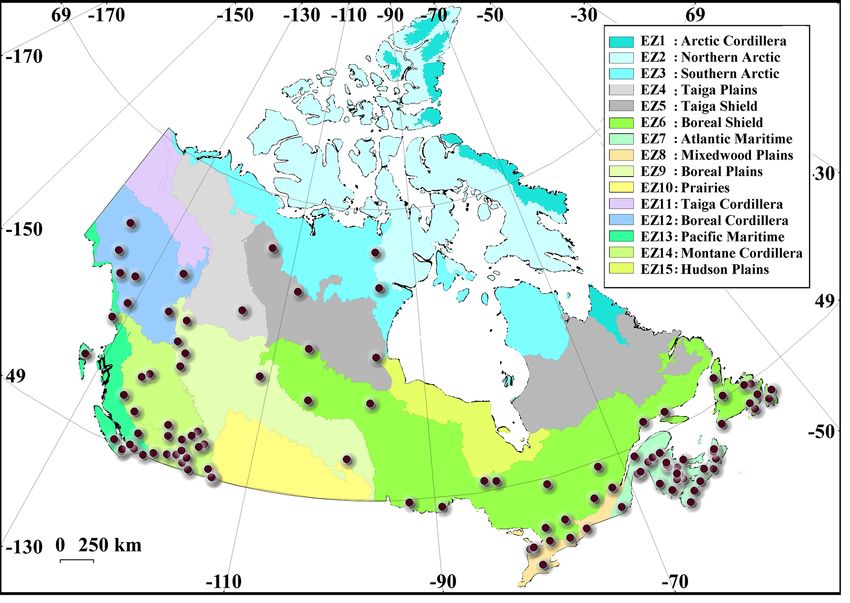
5196                                     M. Zaerpour et al.: A global algorithm for identifying changing streamflow regimes

Figure 1. The workflow of the proposed three-step algorithm for classifying streamflow regime, diagnosing shift in streamflow regime, and
attributing the regime shift to the changes in streamflow characteristics.

2.3    Fuzzy c-means clustering                                        streams into C fuzzy clusters such that the sum of distances
                                                                       for all streams i ∈ {1, . . ., N } between NSFs and cluster cen-
Clustering is the process of arranging data into a finite              troids is minimized. This is often formulated through an it-
set of classes so that members in the same class have                  erative optimization procedure aiming at finding the cluster
similar characteristics. Various statistical methodologies are         centroid by minimizing the generalized least-squared error
used for clustering in hydrology (see Tarasova et al., 2019;           function as the objective of optimization (Bezdek, 1981).
Brunner et al., 2020), often to non-overlapping (i.e., hard)
classes (Olden et al., 2012). Recent theoretical developments                     XC X N      2
have alternatively considered a set of overlapping (i.e., soft)        J U, V|X, Y =   ·   ui,c
classes, in particular in the form of fuzzy clusters (e.g.,                                  c=1 i=1
Knoben et al., 2018; Wolfe et al., 2019). The association                                    2
                                                                                          · d [x i,j =1:n y i,j =1:n ] , vc,m=1:2n

                                                                                                                                            (2a)
to each fuzzy cluster can be quantified using a degree of
membership (see Bezdek, 1981; Sikorska et al., 2015). The
                                                                       This objective function is subject to the following two con-
process of clustering streamflow regime using FCM can be
                                                                       straints:
summarized as the following: assume that streamflow data
from N hydrometric gauges during a common timeframe w                  C
                                                                       X
with the length of l years are available. For each stream,                   ui,c = 1∀i ∈ {1, . . ., N } ,                                 (2b)
the first and
           second   moments
                                  of n IHAs (here n = 15),            c=1
i.e., X = xij Y = yij ; i ∈ {1, . . ., N }, j ∈ {1, . . ., n}, can           N
                                                                             X
be extracted during the initial timeframe w. Before going for-         0<          ui,c < N ∀c ∈ {1, . . ., C} ,                            (2c)
ward, extracted features are normalized to avoid scale mis-                  i=1
matches:

             xi,j − min{xi=1:N,j }                                     where                  V = vc=1:C,m=1:2n = x ∗ c,j =1:n , y ∗ c,j =1:n =
x i,j =                                   ∀j ∈ {1, . . ., n} , (1a)
        max{xi=1:N,j } − min{xi=1:N,j }                                [x ∗ c,1 . . .x ∗ c,n y ∗ c,1 . . .y ∗ c,n ] ∈ R 2n is the matrix of
             yi,j − min{yi=1:N,j }                                     cluster centroids              (i.e., regime types); the matrix of
                                          ∀j ∈ {1, . . ., n} , (1b)

y i,j =                                                                U = ui,c ; i ∈ {1, . . ., N } c ∈ {1, . . ., C} is the matrix           of
        max{yi=1:N,j } − min{yi=1:N,j }
                                                                       memberships; and d2 [x i,j =1:n , y i,j =1:n ], vc,m=1:2n is the


where X = x ij and Y = y ij are the matrices of nor-                   matrix of squared Euclidian distances between NSFs of
malized streamflow features (NSFs). FCM partitions the N               stream i and a cluster’s centroid c. The fuzzy membership

Hydrol. Earth Syst. Sci., 25, 5193–5217, 2021                                               https://doi.org/10.5194/hess-25-5193-2021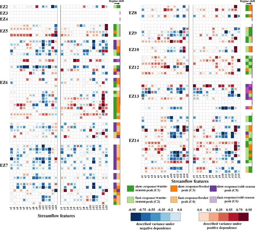
M. Zaerpour et al.: A global algorithm for identifying changing streamflow regimes                                                               5197

matrix can be accordingly calculated as follows:

                                   1
               d2 [x i,j =1:n y i,j =1:n ],vc, m=1:2n
ui,c =                                                          ;
         C

         P                           1
                   d2 [x i,j =1:n y i,j =1:n ],vc, m=1:2n
         c=1
i ∈ {1, . . ., N } , c ∈ {1, . . ., C} .                                     (3)
The number of clusters C (here regime types) can be cho-
sen as a priori or empirically using validity indices (Srini-
vas et al., 2008). Here, we implement three validity indices
of the Xie–Beni index (VXB ; Xie and Beni, 1991), parti-
tion index (VSC ; Bensaid et al., 1996), and separation in-
dex (VS ; Fukuyama and Sugeno, 1989). These indices are
based on two criteria, namely compactness and separation.
The compactness characterizes how close members to each                             Figure 2. A schematic view to the procedure of identifying the
cluster are, whereas the separation measures how distinct                           evolution in membership values using a moving window: (a) a
two clusters are. A good clustering result should have both                         decadal timeframe slides over the streamflow time series year-by-
small intra-cluster compactness and large inter-cluster sep-                        year, and (b) membership degrees are recalculated at each decadal
aration. The Xie–Beni validity index is the ratio of com-                           timeframe to systematically determine the changes in association to
pactness to the separation, quantified by the average of the                        each regime type determined in the beginning of the data period.
fuzzy variation in NSFs from a cluster’s centroid to the mini-
mum squared distance between cluster centroids. Note that
PN          2 2
   i=1 ui,c d      x i,j =1:n , y i,j =1:n , vc,m=1:2n is the com-
pactness of fuzzy cluster c, and separation of fuzzy clusters
is quantified by the minimum squared Euclidean distance be-
tween cluster centroids.                                                            2.4   Detection of change in streamflow regimes
        PC PN               2 2
            c=1 i=1 ui,c d             x i,j =1:n , y i,j =1:n , vc,m=1:2n
VXB =
                                                                                    Clustering natural streams into c regime types takes place
                  N × min d2 vl,m=1:2n , vc,m=1:2n
                                c,l6=c                                              during a baseline timeframe (i.e., the first initial years with
                                                                             (4)    the length of l years), in which the optimal number of clus-
                                                                                    ters, cluster centroids, and initial membership degrees to each
Partition index is quantified by the sum of individual fuzzy
                                                                                    regime type are identified. For each stream, the timeframe
cluster variations (i.e., the compactness of fuzzy clusters) to
                                                                                    can be moved year-by-year, and the membership values can
the sum of the distances from cluster centroids (i.e., the sep-
                                                                                    be recalculated for the new window using Eq. (3). Figure 2
aration of fuzzy clusters). This ratio is further normalized
                                                                                    exemplifies this process in a hypothetical case. This results in
by fuzzy cardinality weight γc , defined by γc = N
                                                    P
                                                        i=1 ui,c ,                  C time series of membership degrees at each stream, show-
to avoid the bias made by cluster sizes.
                                                                                    ing how the association to each regime type evolves in time
                  ( PN             2                                      )
                               ui,c d2 x i,j =1:n , y i,j =1:n , vc,m=1:2n          – see Jaramillo and Nazemi (2018). In order to quantify the

        XC              i=1
VSC =       c=1
                                    Pc 2                                     (5)   gradual change in membership degrees, the Mann–Kendall
                              γc × l=1 d vl,m=1:2n , vc,m=1:2n
                                                                                    trend test with the Sen’s slope is applied (Mann, 1945; Sen,
The separation index, also known as Fukuyama and Sugeno                             1968; Kendall, 1975). As the sum of memberships in each
index, is defined based on the difference between the com-                          timeframe is 1 (see Eq. 2b), a positive trend in memberships
pactness and the separation of fuzzy clusters:                                      to one cluster should coincide with a negative trend in the
VS =
       nXC XN
               u2 .d2 [x i,j =1:n , y i,j =1:n ] , vc,m=1:2n
                                                                     o             membership of at least one other cluster. At each stream, this
       c=1 i=1 i,c                                                                  transition can be identified by significant negative dependen-
     nXC XN                              o
                 2      2                                                           cies between membership degrees.
   −   c=1 i=1
               u i,c .d   [vc,m=1:2n , v    ,                                (6)
                    PC                                                                 Given the pair of clusters p and q in the stream i, the rate
in which v = c=1 vi /c. We identify the optimal number of                           of shift from p to q can be quantified using Eq. (7), where
clusters using the elbow method (see Satopaa et al., 2011;                          ui,p (w) and ui,q (w) are membership degrees to clusters p
Kuentz et al., 2017), which involves finding the maximum                            and q in stream i during the timeframe w, w ∈ {1, . . ., r},
number of clusters, beyond which slopes of improvement in                           r is the number of moving timeframes needed to cover the
validity indices flatten significantly, and adding a new cluster                    whole data period year-by-year, E(ui,p ) and E(ui,q ) are the
does not justify the increased complexity.                                          expected memberships, and Si, (p,q) is the slope of the best-

https://doi.org/10.5194/hess-25-5193-2021                                                         Hydrol. Earth Syst. Sci., 25, 5193–5217, 2021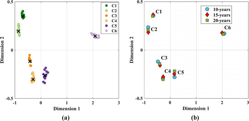
5198                                                     M. Zaerpour et al.: A global algorithm for identifying changing streamflow regimes

fitted line.                                                                                 in streamflow characteristics. Figure 4 shows this integration
                 m
                 P                                                                       using a hypothetical example. Figure 4a demonstrates a mul-
                         ui,q (w) − E ui,q             ui,p (w) − E ui,p                     tifaceted change in the shape of the annual hydrograph in a
                w=1                                                                          given stream during two separate periods, shown with grey
Si,(p,q) =                        m                            2
                                                                                       (7)
                                  P
                                        ui,q (w) − E ui,q                                    and pink envelopes. The black and red lines are expected an-
                                  w=1                                                        nual hydrographs for each envelope (i.e., the mean of annual
                                                                                             streamflow hydrographs over the timeframe). Any shift be-
                                                                                             tween flow regimes is described by at least a pair of mem-
2.5     Attribution of change in streamflow regime to                                        bership time series with opposite trends. The strength of the
        alterations in streamflow characteristics                                            link is measured using R 2 . Figure 4b shows the rates of shifts
                                                                                             and the attribution to changes in streamflow characteristics.
Here, the existence of significant dependence between mem-
                                                                                             The thickness of links is proportional to rates of shift and/or
bership values and streamflow features is taken as the ba-
                                                                                             R 2 values.
sis for attribution. Accordingly, we use Kendall’s tau (Gen-
est and Favre, 2007; Nazemi and Elshorbagy, 2012) to de-
tect the co-occurrence between changes in memberships and
                                                                                             3   Case study and data
changes in NSFs. Figure 3 shows the procedure of attribu-
tion. Left panels show the changes in membership degrees of
                                                                                             With a total drainage area equivalent to 6 % of the global land
two hypothetical clusters (purple lines), along with the cor-
                                                                                             area, Canadian rivers support important socio-economic ac-
responding changes in two NSFs (grey lines). Right panels
                                                                                             tivities such as agriculture and hydropower production. River
show the scatter plots of membership degrees vs. the NSFs.
                                                                                             systems in Canada can be divided into four major ocean-
We identify the significance and the direction of dependence
                                                                                             drained basins, namely Pacific, Atlantic, Arctic, and Hud-
using Kendall’s tau coefficient. To measure the linear associ-
                                                                                             son Bay that can be further divided into a number of sub-
ation between changes in streamflow features xi,j and mem-
                                                                                             basins (Pearse et al., 1985; Natural Resources Canada, 2007).
bership values ui,c , the coefficient of determination (R 2 ; see
                                                                                             The Pacific basin, the smallest among all, spreads along the
Legates and McCabe, 1999) is used. R 2 varies between [0,
                                                                                             west coast from the US border to Yukon and drains around
1] and determines how much of the variability in the degrees
                                                                                             1 million km2 . The main sub-basins in the Pacific include
of membership can be described by the variability in a given
                                                                                             Fraser, Yukon, Columbia, and the Seaboard. In the east coast,
streamflow characteristic. The greater the R 2 is, the stronger
                                                                                             the Atlantic basin drains a total area of 1.6 million km2 and
the association between changes in degrees of membership
                                                                                             includes important water bodies such as the Great Lakes. The
and the streamflow characteristics is. The coefficient of de-
                                                                                             basin includes three sub-basins, namely the St. Lawrence
termination can be calculated as follows:
                                                                                             River, Seaboard, and the Saint John-St. Croix. Towards the
                           r
                            P
                                                                            2
                                                                                             north, the Arctic basin drains over 3.5 million km2 of north-
                                  ui,c − E ui,c        xi,j − E xi,j
                            w=1
                                                                                             ern lands and includes some of Canada’s largest lakes other
R 2 ui,c , xi,j =

                        r
                        P                         r
                                              2 P                         2              than the Great Lakes such as the Slave, Athabasca, and Great
                              ui,c − E ui,c              xi,j − E xi,j
                        w=1                       w=1                                        Bear lakes. The Mackenzie, Peace–Athabasca, and Seaboard
∀i ∈ {1, . . ., N } .                                                                  (8)   are the main sub-basins in the Arctic basin. With an area of
                                                                                             3.8 million km2 , Hudson Bay is the largest drainage basin in
By the simultaneous use of Kendall’s tau and R 2 , we try to fa-                             Canada, covering five provinces from Alberta in the west to
cilitate quantitative communication of the impact of changes                                 Québec in the east. The basin includes four major sub-basins,
in a specific streamflow characteristic on the transition from                               namely Western and Northern Hudson Bay, Nelson, North-
one regime type to another. By using Kendall’s tau, we                                       ern Ontario, and Northern Québec. Nelson, Saskatchewan,
identify the sign and significance of dependencies between                                   and Churchill rivers are the major river systems in Hudson
changes in membership degrees and streamflow characteris-                                    Bay.
tics using a non-parametric approach that can handle non-                                       Natural streamflow regimes in Canada have undergone
linearity in the form of association. Using R 2 , we quantify                                drastic changes in recent years which are expected to in-
how much of the variability in the membership degrees can                                    crease under future climate change conditions (Woo et
be described by the variability in the changes in streamflow                                 al., 2008). Observed and projected changes in streamflow
characteristics. This is to provide a comprehendible measure                                 regimes are not only between different regions (Kang et
of association between the two quantities. As R 2 is a linear-                               al., 2016; Islam et al., 2019), but they also occur within
based measure, we repeat the experiment by replacing the                                     the same ecological and/or hydrological regions (Whitfield,
R 2 with squared Kendall’s tau and discuss the uncertainty                                   2001; Whitfield et al., 2020). For instance, there are sig-
in our attribution. The key advantage of our proposed algo-                                  nificant differences among forms of change in streamflow
rithm is in providing a workflow in which the detection of a                                 regimes between the northern and southern Pacific (Kang
change in streamflow regime is directly attributed to changes                                et al., 2016; Brahney et al., 2017). Similarly, glacier-fed

Hydrol. Earth Syst. Sci., 25, 5193–5217, 2021                                                                 https://doi.org/10.5194/hess-25-5193-2021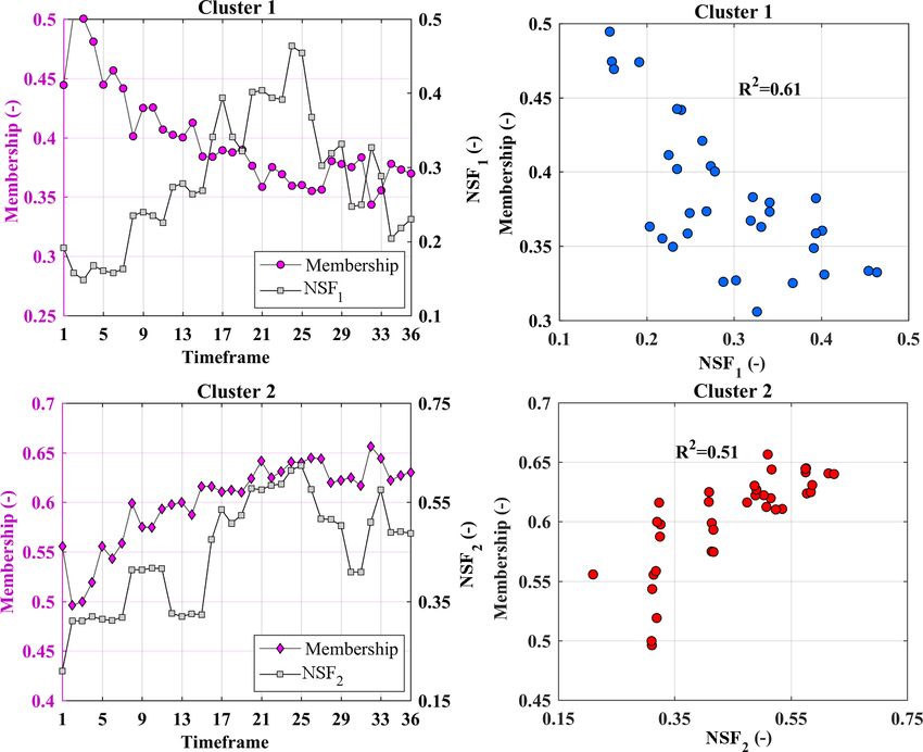
M. Zaerpour et al.: A global algorithm for identifying changing streamflow regimes                                                         5199

Figure 3. The procedure of attributing changes in membership degrees to changes in streamflow characteristics. The left column shows the co-
evolution of membership degrees and normalized streamflow features (i.e., NSF1 and NSF2 ). The right column measures the correspondence
between changes in membership degrees and normalized streamflow features through percentage of described variance quantified using R 2 .
Red and blue dots show the positive and negative dependencies, respectively.

Figure 4. An example for transitions between regime types along with attribution of change to streamflow characteristics. Panel (a) shows
annual hydrographs in two separate periods using grey and pink envelopes. Panel (b) shows the dominant shift in the flow regime by maximum
rate of shift and attributes this shift to changes in significantly dependent streamflow characteristics. The dominant shift is visualized by the
thickest grey envelope. The strength of the association between regime shift and significantly dependent streamflow characteristics are
measured and communicated by R 2 .

rivers in northern Canada show increases in summer runoff                  mate change impacts on natural streamflow regimes (Brim-
(Fleming and Clarke, 2003), whereas other rivers show a                    ley et al., 1999; Harvey et al., 1999). In the period of 1903 to
tendency toward decreasing summer runoff (Fleming and                      2015, we search for the largest subset of hydrologically un-
Clarke, 2003; Janowicz, 2008, 2011). To diagnose simultane-                connected stations with the longest continuous daily record
ous changes in natural streamflow regimes across Canada, we                during a common period and less than a month worth of
use the data from the Reference Hydrometric Basin Network                  missing data in a typical year. This results in selecting 105
(RHBN; Water Survey of Canada, 2017, http://www.wsc.ec.                    streamflow stations during the water years of 1966 to 2010
gc.ca/, last access: August 2020). RHBN includes 782 Cana-                 (1 October 1965 to 30 September 2010).
dian hydrometric stations that measure streamflow at unreg-                   Although drainage basins are often used as the spatial unit
ulated tributaries and are particularly suitable to address cli-           in which alteration in streamflow regimes is investigated,

https://doi.org/10.5194/hess-25-5193-2021                                                 Hydrol. Earth Syst. Sci., 25, 5193–5217, 2021
5200                                  M. Zaerpour et al.: A global algorithm for identifying changing streamflow regimes

there are substantial differences within a drainage basin in      (EZ15) includes 4 % of Canada in the southern part of Hud-
terms of climate, topography, vegetation, geology, and land       son Bay with a large number of wetlands. Table 2 summa-
use. This results into multiple forms of hydrological re-         rizes the selected stations within each ecozone.
sponses within one drainage basin. In contrast to drainage           Tables S1 to S4 in the Supplement introduce these sta-
basins, terrestrial ecozones are identified based on similarity   tions across the four drainage basins in Canada. Figure 5
in climate and land characteristics, and therefore, they can      shows the distribution of the selected stations across the 15
be more representative of different hydrological responses        ecozones. As is clear, the density of selected stations varies
(Whitfield, 2001). In brief, an ecozone is a patch of land        greatly among ecozones. The highest numbers of stations
with distinct climatic, ecologic, and aquatic characteristics     are within Atlantic Maritime, Boreal Shield, and Montane
(see Wiken, 1986; Marshall et al., 1999; Wong et al., 2017).      Cordillera, while the southern and northern Arctic, as well
Canada includes 15 ecozones. Starting from the north, the         as Taiga Plains, include only one; and there is no station in
Arctic Cordillera (EZ1), covering 2 % of Canada’s landmass,       the Arctic Cordillera, Taiga Cordillera, and Hudson Plains.
contains the only major mountainous region in Canada other        At the basin/sub-basin scale, the selected stations cover all
than the Rockies. The Northern Arctic (EZ2) is equivalent to      14 main Canadian sub-basins – see Table S5 and Fig. S1 in
14 % of Canada’s landmass and covers Arctic islands (Coops        the Supplement.
et al., 2008). The Southern Arctic (EZ3) includes the north-
ern mainland, covering 8 % of Canada. The Taiga Plains
(EZ4) extends mainly on the western side of the North-            4     Results
west Territories, covers 6 % of Canada’s landmass, and in-
cludes a large number of wetlands. Taiga Shield (EZ5), with       We apply the framework proposed in Sect. 2 to the selected
a large number of lakes, covers 13 % of Canada’s landmass         RHBN streams. At each stream, we first convert the daily
in the south of the southern Arctic (Marshall et al., 1999).      discharge data into runoff depth in millimetres per week and
The Boreal Shield (EZ6) is Canada’s largest ecozone cover-        calculate the thirty streamflow features introduced in Table 1.
ing 18 % of the country’s landmass, extending from north-         We then consider a multi-year timeframe for clustering and
ern Saskatchewan toward the south into Ontario and Québec         assigning initial membership values. The length of this time-
and then northward toward eastern Newfoundland (Rowe and          frame should be chosen in a way that (1) provides a notion
Sheard, 1981). The Atlantic Maritime (EZ7) includes the Ap-       for streamflow regime and (2) provides enough timeframes
palachian mountain region, covering 2 % of Canada and ex-         to assess evolution in membership values. As the aim is to
tending from the mouth of the St. Lawrence River and Bay          address temporal changes in the streamflow regime, the base-
of Fundy to coastlines of New Brunswick, Nova Scotia, and         line timeframe is considered at the beginning of the stream-
Prince Edward Island. The Mixedwood Plains (EZ8) is the           flow time series. Here, we present our result based on con-
most southerly ecozone, covering 2 % of Canada, but in-           sidering decadal timeframes and the period of 1966 to 1975
cludes the country’s most populated regions in Ontario and        as the baseline. We address and discuss the sensitivity of our
Québec. The Boreal Plains (EZ9) covers 7 % of Canada’s            results to these assumptions in Sect. 5.
landmass in western Canada, from British Columbia to the
southeastern corner of Manitoba in the south of the Bo-           4.1    Identifying natural streamflow regimes in Canada
real Shield (Ireson et al., 2015). The Prairies (EZ10) ex-
tend from south-central Alberta to southeastern Manitoba,         We attempt to find the optimal number of clusters empiri-
covering 5 % of Canada’s landmass and the majority of             cally from the pool of c = {2, 3, . . ., 10}, using the three va-
Canada’s agricultural lands (Nazemi et al., 2017). The Taiga      lidity indices introduced in Sect. 2.3. Figure S2 in the Supple-
Cordillera (EZ11) includes 3 % of Canada with the least           ment shows the result of this investigation, indicating the op-
amount of Canada’s forest and lies along the northern portion     timal number of clusters as c = 6, in which decreasing slopes
of the Rocky Mountains (Power and Gillis, 2006). The Bo-          of the three validity indices flatten. To provide a sense of
real Cordillera (EZ12) covers 5 % of Canada from northern         these streamflow regimes and their changes in time, we vi-
British Columbia to the southern Yukon, with mountainous          sualize the shapes of annual streamflow hydrographs in the
uplands and forested lowlands. The Pacific Maritime (EZ13)        archetype streams during the baseline and the last decadal
mainly includes the coastal mountains of British Columbia         timeframe (i.e., 1966 to 1975 vs. 2001 to 2010) in Fig. S3
and lands adjacent to the Pacific coast, having the warmest       in the Supplement. Archetype streams are those streams that
and wettest climate in the country, in an area around 2 %         have the highest association with the identified regime types
of Canada (Wiken, 1986). The Montane Cordillera (EZ14),           and can represent the characteristics of a given regime better
with the most diverse climate in Canada, includes 5 % of          than other members of the cluster. Table 3 introduces these
Canada in mountainous areas of southern British Columbia          six regimes along with their notation and archetype streams.
and southwestern Alberta and provides headwater flow to           We name clusters based on two key characteristics, i.e., the
some important river systems such as Fraser, Saskatchewan,        form of hydrologic response (i.e., fast vs. slow response) and
and Athabasca (Marshall et al., 1999). Finally, Hudson Plains     the timing of the annual peak flow (i.e., cold-season, freshet,

Hydrol. Earth Syst. Sci., 25, 5193–5217, 2021                                      https://doi.org/10.5194/hess-25-5193-2021
M. Zaerpour et al.: A global algorithm for identifying changing streamflow regimes 5201
Table 2. List of Canadian ecozones with at least one RHBN station in this study, along with their abbreviations and the number of RHBN
stations considered within each ecozone.
Abbreviation Ecozones No. of stations Abbreviation Ecozones No. of stations
EZ2 Northern Arctic 1 EZ8 Mixedwood Plains 5
EZ3 Southern Arctic 1 EZ9 Boreal Plains 6
EZ4 Taiga Plains 1 EZ10 Prairies 2
EZ5 Taiga Shield 4 EZ12 Boreal Cordillera 7
EZ6 Boreal Shield 25 EZ13 Pacific Maritime 9
EZ7 Atlantic Maritime 25 EZ14 Montane Cordillera 19
Figure 5. The distribution of the selected 105 RHBN streamflow stations within the Canadian ecozones.
and warm-season peaks). The form of hydrologic response terized by a gradual rise after spring snowmelt, prolonged
can be proxied by variability in the annual streamflow hy- peak discharge throughout summer, gradual recession during
drograph. The greater the variability in the annual streamflow fall, and low runoff in winter (Déry et al., 2009). Streams
hydrograph is, the faster the hydrologic response is. belonging to C1 spread mostly in northwestern Canada and
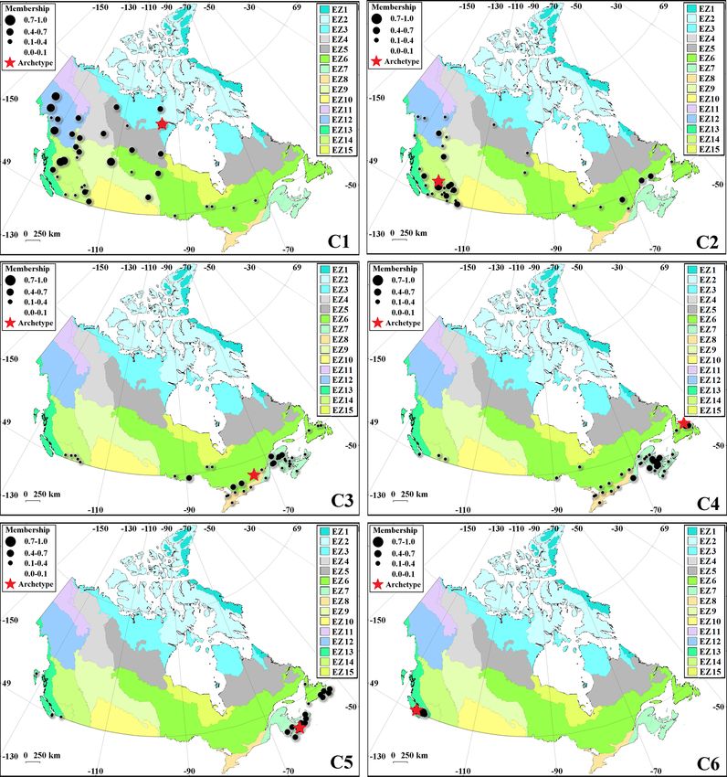
Figure 6 shows a synoptic look at the distribution of are either glacial-fed or lake-dominated streams, in which
streams belonging to each flow regime during the initial base- the hydrologic responses are delayed due to the slow rate of
line timeframe. In each panel, the red star represents the glacial retreats and/or storage effects of large in-stream lakes.
archetype stream, and streams with membership values of The Kazan River releasing into Baker Lake in Nunavut is
0.1 and larger are shown with circles. The larger the size of a the archetype stream for this regime type. C2 is very similar
circle is, the greater the degree of membership to each cluster to C1, however with greater variability in annual streamflow
is. As Fig. 5 shows, the six clusters are geographically identi- hydrographs. The streams belonging to this stream type are
fiable and resemble some of the already-known regime types mainly concentrated in western Canada, particularly in the
across the country (see Whitfield, 2001; Bawden et al., 2015; Montane Cordillera (46 % of streams), and include streams
Burn and Whitfield, 2016; Bush and Lemmen, 2019). that are fed mainly through snow and glacial melts (Eaton
The “slow-response/warm-season peak” regime, i.e., clus- and Moore, 2010; Moore et al., 2012; Schnorbus et al., 2014).
ter C1, includes streams with strong seasonality, high dis- There are, however, streams belonging to C2 that are located
charge in summer, and smaller variability in annual stream- in the Boreal Shield (23 % of streams), where the streamflow
flow hydrograph compared to cluster C2, i.e., the “fast- generation is governed by other processes such as fill-and-
response/warm-season peak” regime. Cluster C1 is charac- spill in which segments of a basin have to be filled above
https://doi.org/10.5194/hess-25-5193-2021 Hydrol. Earth Syst. Sci., 25, 5193–5217, 20215202 M. Zaerpour et al.: A global algorithm for identifying changing streamflow regimes
Table 3. Six identified regime clusters along with their labelled regime type and archetype stream.
Cluster Regime type Archetype (representative) stream
C1 Slow-response/warm-season peak Kazan River above Kazan Falls (HYDAT ID: 06LC001)
C2 Fast-response/warm-season peak Clearwater River near Clearwater Station (HYDAT ID: 08LA001)
C3 Slow-response/freshet peak Matawin River at Saint-Michel-des-Saints (HYDAT ID: 02NF003)
C4 Fast-response/freshet peak Gander River at Big Chute (HYDAT ID: 02YQ001)
C5 Slow-response/cold-season peak Beaver Bank River near Kinsac (HYDAT ID: 01DG003)
C6 Fast-response/cold-season peak Sproat River near Alberni (HYDAT ID: 08HB008)
their capacity before spillage (Spence and Phillips, 2015). 2001). Streams belonging to this regime are only concen-
The Clearwater River near Clearwater in southern Alberta trated in the Pacific. The Sproat River near Alberni is the
is the representative stream for this regime type. archetype stream of the C6 cluster.
The cluster C3, i.e., the “slow-response/freshet peak”
regime, includes streams in which the annual streamflow vol- 4.2 Detection of changing streamflow regimes
ume is mainly contributed by a short high-flow period dur-
ing spring snowmelt, sharp recession in summer, yet rela- To understand temporal shifts in streamflow regimes
tively smaller variations in the shape of hydrograph com- throughout selected RHBN streams, we calculate the decadal
pared to the cluster C4, i.e., “fast-response/freshet peak” membership values as shown in Fig. 2. We accordingly ap-
regime. Nearly 45 % of the streams with this regime type are ply the Mann–Kendall trend test with the Sen’s Slope on the
located in Atlantic Maritime. The rest are distributed in the time series of decadal memberships. The detailed results in-
Boreal Shield (28 %), Mixedwood Plains (15 %), and Mon- cluding the membership time series for all streams and corre-
tane Cordillera (12 %). The Matawin River originating from sponding trend analyses are shown in Figs. S4 and S5 in the
lake Matawin in Québec is the archetype for the C3 regime. Supplement over major drainage basins/sub-basins and the
The streams belonging to C4 are also dominated by spring terrestrial ecozones in Canada, respectively. Figure 7 summa-
snowmelt but showing more variation in the shape of annual rizes our findings over the 15 Canadian ecozones. The colour
hydrographs compared to the C3 regime. Streams belonging (blue vs. red) and the size (large vs. small) of triangles show
to the C4 regime often have two distinct peaks, one in spring decreasing vs. increasing trends, as well as significant vs. in-
induced by snowmelt and one in fall due to high precipita- significant trends at p value ≤ 0.05. Although inconsistent
tion, and from that sense, they largely resemble nival–pluvial patterns of change are observed in the Boreal and Montane
streams (Hock et al., 2005). Almost all streams belonging to cordilleras, particularly between the southern and northern
the C4 regime are located in eastern Canada (50 % in Atlantic regions, there are clear downward trends in the member of
Maritime, 26 % in the Boreal Shield, 16 % in Mixedwood regime C1 in the Taiga Shield and Boreal Shield. Upward
Plains). Gander River at Partridgeberry Hill in Newfound- trends are observed in membership values of C2 in the Bo-
land is the archetype for this regime. real Cordillera and Taiga Shield, while downward trends are
The cluster C5, i.e., “slow-response/cold-season peak” seen in the member of C2 in southern and eastern parts of
regime, comprises streams with weak seasonality and the Montane Cordillera and Boreal Shield. The C3 regime
slightly more discharge in fall and winter. The annual flow shows intensification in the Montane Cordillera and Boreal
for streams belonging to this regime is more influenced by Shield. It also intensifies in southern parts of Atlantic Mar-
rainfall around late fall, followed by a slight increase in itime but weakens in northern regions. The pattern of change
discharge due to snowmelt; therefore, they resemble a hy- in C4 is very similar to C3 but with fewer significant down-
brid pluvial–nival regime (Kang et al., 2016). The concen- ward trends in northern parts of Atlantic Maritime. Consider-
tration of streams belonging to this regime is again in east- ing the C5 regime, streams mainly show decreasing trends in
ern Canada (48 % in Atlantic Maritime; 33 % in the Bo- the Appalachian region including the eastern Boreal Shield
real Shield), with a few streams being in the Pacific Mar- and southern parts of Atlantic Maritime. Mixed patterns of
itime. Beaver Bank River in Nova Scotia is the representative change in membership degree are observed in the Pacific
stream for this regime type. Finally, the cluster C6, i.e., “fast- Maritime for both C5 and C6 regimes.
response/cold season peak regime, is similar to the C5 regime The nature of regime shifts at each stream can be investi-
and exhibits a weak seasonality but with a greater variation gated by quantifying the rate of relative shift between oppos-
in shapes of annual hydrographs. The runoff in streams be- ing significant trends. Figure S6 in the Supplement summa-
longing to this regime is dominated by heavy precipitation, rizes the results. Overall, the dominant modes of transition
especially during winter, and lower runoff during summer, at the ecozone scale are from C1 to C2 in the northern eco-
resembling the pluvial regime (Wade et al., 2001; Whitfield, zones (EZ5 and EZ12), from C2 to C1 and from C2 to C3
in the western ecozones (EZ9 and EZ14), from C2 to C3 at
Hydrol. Earth Syst. Sci., 25, 5193–5217, 2021 https://doi.org/10.5194/hess-25-5193-2021M. Zaerpour et al.: A global algorithm for identifying changing streamflow regimes 5203 Figure 6. The distribution of the identified regime types across Canadian ecozones during the baseline l timeframe of 1966 to 1975. Each stream is represented by a circle with a radius proportional to a membership degree quantifying the association to a given regime type. Only RHBN stations with degrees of membership of 0.1 or larger are shown in each panel. The red stars are the archetype stations related to each regime type. the two stations located in the Prairies, from C1 to C3 in our findings in Canada and highlight dominant regime shifts the eastern ecozones (EZ6, EZ8, and EZ15), and from C5 and their geographic extent across the country, Fig. 8 shows to C4 in the Appalachian region (EZ7 and eastern part of Sankey diagrams demonstrating the initial regime types in EZ6). The variability between the regime shifts inside each the considered streams. Streams are grouped by the ecozones ecozone can be described by elevation. To better synthesize on the left side of each panel and transform to one particular https://doi.org/10.5194/hess-25-5193-2021 Hydrol. Earth Syst. Sci., 25, 5193–5217, 2021
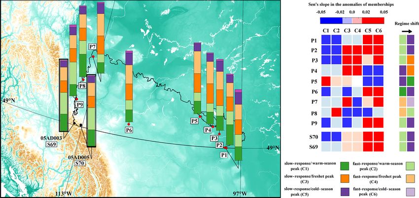
5204                                   M. Zaerpour et al.: A global algorithm for identifying changing streamflow regimes

Figure 7. Trends in decadal memberships, quantifying the change in association of the 105 selected RHBN streams to the six regime types
during 1966 to 2010.

target regime type (right side of each panel). The six natural           Some important findings can be made from Fig. 8. While
regime types are distinguished by colour codes, and stations          regime shifts are varied, there are some dominant regime
within each ecozone are sorted from the lowest to the highest         shifts that are frequently observed across different ecozones.
elevation from top to the bottom. The width of each arrow             For example, frequent shifts are observed from C2 to C1, as
is proportional to the rates of shift, calculated using Eq. (7).      well as C1 to C2, that are quite strong across the Montane
The highest rate of a shift in each stream and/or ecozone can         Cordillera and Taiga Shield, respectively. Second, it is pos-
be considered as the dominant regime shift.                           sible that the streamflow regime in a given ecozone shifts

Hydrol. Earth Syst. Sci., 25, 5193–5217, 2021                                          https://doi.org/10.5194/hess-25-5193-2021
M. Zaerpour et al.: A global algorithm for identifying changing streamflow regimes                                                     5205

Figure 8. Sankey diagrams showing transitions in Canadian natural streamflow regimes described across ecozones from 1966 to 2010.
Each panel presents the transformation from five potential regime types to one particular target regime. Streams in the left side are grouped
according to ecozones and are sorted from the lowest to highest elevations from the top to the bottom. Colours show the six regime types.
The widths of arrows are proportional to the rate of shift.

from one regime to two or more regime types. For instance,               4.3   Identifying forms of transformation in streamflow
streamflow in Atlantic Maritime shifts from C5 to C3 and                       regimes
C4. Also, it is possible to have opposing regime shifts in a
given ecozone. As an example, the flow regime varies from
C5 to C6 and vice versa across Pacific Maritime. Such vari-              The procedure presented in Sect. 2.5 attributes regime shifts
abilities in regime shift can be partially explained by lati-            to changes in streamflow characteristics using dependence
tude. More generally, it is possible to shift from two or more           analysis. Figure 9 summarizes the results of attribution for
regime types into one or more regime types across a partic-              the 105 RHBN stations. Streams are shown in rows, grouped
ular ecozone. For example, streams with C1 and C5 regimes                in each ecozone, and ordered from low to high elevations
are shifting to C3 and C4 across the Boreal Shield. Such vari-           from the top to the bottom. For each stream, there are three
abilities within an ecozone can be described in many cases by            groups of cells, with 15, 15, and 2 cells from left to right.
elevation. In the Boreal Shield, for example, elevation con-             The first two groups of cells are related to the values of
trols the constitution of the initial streamflow regime from             mean (i.e., x1 to x15 ) and variance (i.e., y1 to y15 ) of the
C5 in lowlands to C1 in highlands. Finally, the most frequent            15 considered IHAs. In these two groups of cells, shades of
regime shifts are not necessarily the strongest ones. For in-            blue and red show negative and positive dependencies be-
stance, the streamflow regime shifts across six ecozones to-             tween a given pair of streamflow characteristic and member-
ward C3 and C4, but the rates of the shift are not strong when           ship degree, respectively. Note that we only identify those
compared with the shift between C6 to C5 that happens in                 streamflow characteristics that have significant dependencies
limited streams in Pacific Maritime, but quite strong.                   with variations in membership degrees based on Kendall’s
                                                                         tau (p value ≤ 0.05) Colour saturations show the values for
                                                                         the coefficient of determination, quantifying the fraction of

https://doi.org/10.5194/hess-25-5193-2021                                              Hydrol. Earth Syst. Sci., 25, 5193–5217, 2021
5206 M. Zaerpour et al.: A global algorithm for identifying changing streamflow regimes
variability in membership degrees that are described by the monthly flow in February, March, and April, more variability
variability in streamflow characteristics. The last two cells in the timing of the low flow, and decreasing September flow.
are related to the dominant regime shift in each stream from
one initial regime (left hand cell) to an altered regime (right
hand cell). The colour scheme, defining the regime types, is 5 Discussion
shown in the legend. The analyses over basin and sub-basin
scales are presented in Figs. S7 and S8 in the Supplement. The application of the proposed methodology in Canada
The most important observation is the fact that in more identifies six distinct natural regimes across the country, ad-
than 80 % the considered natural streams, there are some dress their change in time and space, attribute dominant
identifiable regime shifts that are significantly dependent on regime shifts to changes in a range of streamflow character-
the changes in the streamflow characteristics. Some dom- istics at each stream, and accordingly upscale the findings
inant regime shifts are frequent within an ecozone, while from individual streams to ecozones. Having said that, still
some are less frequent and may depend on latitude and/or there are some unanswered questions. First, it is still unclear
elevation. In the only considered stream in the Northern Arc- how robust our proposed algorithm is particularly in light
tic Ecozone, the shift from the C2 to the C1 regime is at- of the assumptions made with respect to the length of the
tributed to the earlier and more variable timing of the annual timeframes and/or selecting the baseline period. Second, it is
low flow, as well as the increasing June flow. An opposing obvious that our selected streams are only a sample of avail-
shift is observed in Taiga Shield, i.e., from C1 to C2, which able RHBN stations across Canada, and it is still unclear how
can be attributed to the earlier and more variable timing of our findings can be extended to out-of-sample streams. Fi-
annual high flow, as well as the increasing seasonal flow in nally, there is a large body of literature reporting shifts in
fall. The regime shift from C5 to C4 in the lowlands of the streamflow regimes across different regions in Canada due
Boreal Shield is attributed to the decreasing mean of and vari- to changes in temperature patterns, magnitude and form of
ance in annual flow particularly in August. In the highland of precipitation, and snowmelt and snow accumulation, as well
this ecozone, however, the dominant regime shift is from C1 as glacier retreat and permafrost degradation. Accordingly, it
to C3 and can be attributed to the decreasing monthly flow in is crucial to frame and position our findings with respect to
August and September, as well as more variability in the tim- earlier studies. These three tasks are pursued in this section.
ing of the annual low flow. In Atlantic Maritime, particularly
across lowlands, decreasing mean of and variation in the flow 5.1 Addressing uncertainty
in August along with decreasing monthly flow in June and
July, as well as decreasing mean annual and seasonal flow in The results presented in Sect. 4 are based on decadal time-
the fall, lead to a shift from C5 to C4. frames and the selection of the first decadal timeframe as
In Mixedwood Plains, the shift from C1 to C3 is attributed the baseline period. Here we relax these two assumptions
mainly to the earlier and more variable timing of annual low and monitor alterations in our findings. First, we repeat the
flow. In the lowlands of Boreal Plains, the increasing varia- clustering algorithm over all possible decadal timeframes
tion in April’s flow and decreasing annual and summer flows throughout the study period and recalculate the cluster cen-
contribute to the shift from C2 to C1. Streams in the high- ters. This experiment addresses the sensitivity of our clus-
lands of Boreal Plains, however, shift from C1 to C2 due tering algorithms to the choice of baseline period. Second,
to the increasing annual and summer flows, along with the we repeat the approach implemented in Sect. 4 again with
later and more variable timing of low flows. In the Prairies, 15- and 20-year timeframes and address how cluster cen-
in the two considered streams, the shift from C2 to C3 is at- ters, as well as our specific findings, would be altered by
tributed to the delayed and more variable timing of low flows increasing the length of timeframe. We do not consider time-
and decreasing summer flows. In the Boreal Cordillera, more frames less than decadal length due to the insufficiency of
variable annual flow and increasing mean of and variation in numbers of data points for trend analysis. We also do not
May flow correspond to the shift from C1 to C2. Opposing consider timeframes larger than 20 years to allow there to be
shifts from C2 to C1, however, are mainly attributed to the in- at least two fully independent timeframes during the study
creasing monthly flows in February, March, April, and May. period with a gap of a few years. Figure 10 summarizes
The most pronounced shift in Pacific Maritime is from C5 our findings in terms of the sensitivity of our clustering re-
to C6, which mainly corresponds to increasing mean of and sults with respect to the two assumptions made. Panel (a)
variation in October flow, as well as increasing annual flows. shows the cluster centers when different decadal baselines
The most pronounced shift in the Montane Cordillera is from are considered. Coloured dots show the centers of clusters
C2 to C1 for the streams in the northern part, attributed to de- related to all possible decadal timeframes except the period
creasing mean of and variability in July flow and increasing of 1966 to 1975. The centers of clusters are scaled into two
monthly flow in April and May. Streams in southern parts, dimensions using multidimensional scaling (MDS; Cox and
however, shift from C2 to C3, attributed mainly to increasing Cox, 2008), in which the distance between the dots repre-
sents the approximate dissimilarity of centers of clusters.
Hydrol. Earth Syst. Sci., 25, 5193–5217, 2021 https://doi.org/10.5194/hess-25-5193-2021M. Zaerpour et al.: A global algorithm for identifying changing streamflow regimes 5207
Figure 9. Dominant regime shifts across 105 RHBN streams in Canada attributed to the first and second moments of the 15 IHAs considered.
Shades of red and blue show the positive and negative dependencies between changes in streamflow features and degrees of membership.
Colour saturations are proportional to the values of the coefficient of determination. The dominant regime shift at each stream is identified
by the colour scheme described in the legend. Streams are grouped in ecozones and ordered from low (top) to high (bottom) elevations.
Dimensions 1 and 2 delineate the space in which the orig- We also look at possible differences in the direction of
inal data are mapped. Black crosses show the centers of the trends in membership degrees, dominant regime shifts, and
first decadal timeframe mapped using MDS. Colours identify the attribution to streamflow features at the basin scale if the
regime types. The result clearly shows that despite changing length of timeframes are changed. Figure 11 (left column)
the baseline timeframe, the distinctions between cluster cen- intercompares the results obtained by 10-, 15-, and 20-year
ters are maintained, and the position of centers does not sub- timeframes in terms of percentages of similarities in the di-
stantially change by changing the baseline period. Panel (b) rection of trends during 1966 to 2010 at each basin. In brief,
shows the results of our sensitivity analysis with respect to there is at least 80 % agreement between the results obtained
changing the length of timeframe. Again, there are not no- in the Pacific and the Arctic basins. There are more discrep-
table changes in the cluster centers. These two findings high- ancies in the direction of trends in the Atlantic and Hudson
light the robustness of our clustering analysis. Bay basins. This is particularly the case for the C1 regime in
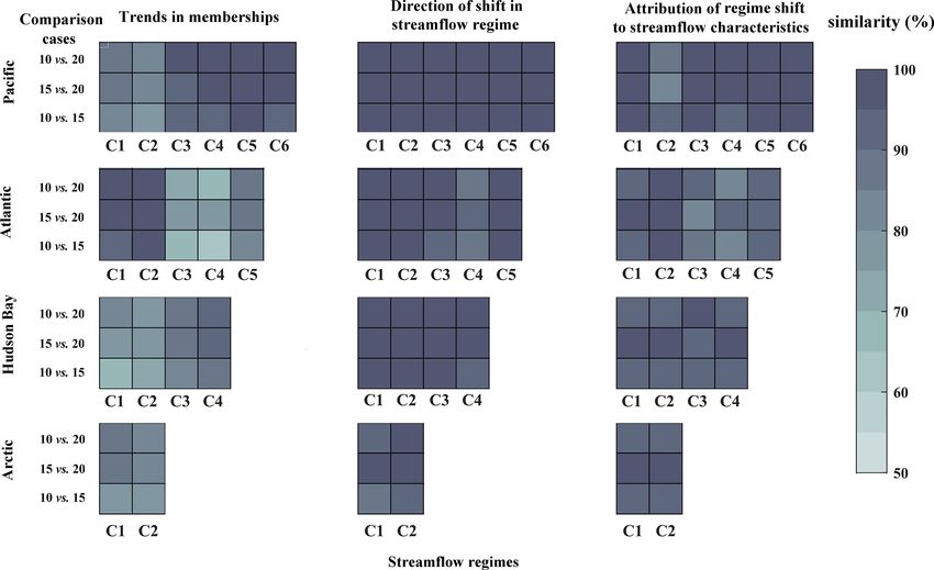
Hudson Bay and for the C3 and C4 regimes in the Atlantic,
https://doi.org/10.5194/hess-25-5193-2021 Hydrol. Earth Syst. Sci., 25, 5193–5217, 2021You can also read