THEMA Working Paper n 2021-16 CY Cergy Paris Université, France Modelling Ridesharing in a Large Network with Dynamic Congestion - August 14, 2021
←
→
Page content transcription
If your browser does not render page correctly, please read the page content below
THEMA Working Paper n°2021-16
         CY Cergy Paris Université, France

Modelling Ridesharing in a Large Network with
            Dynamic Congestion

   André de Palma, Lucas Javaudin, Patrick Stokkink, Léandre Tarpin‐Pitre

                          August 14, 2021
Modelling Ridesharing in a Large Network with Dynamic Congestion

                  André de Palma1 , Lucas Javaudin1 , Patrick Stokkink2 , Léandre Tarpin-Pitre2

Abstract

In ridesharing, commuters with similar itineraries share a vehicle for their trip. Despite its clear benefits
in terms of reduced congestion, ridesharing is not yet widely accepted. We propose a specific ridesharing
variant, where drivers are completely inflexible. This variant can form a competitive alternative against
private transportation, due to the limited efforts that need to be made by drivers. However, due to this
inflexibility, matching of drivers and riders can be substantially more complicated, compared to the situation
where drivers can deviate.
   In this work, we identify the effect of such a ridesharing scheme on the congestion in a real network of
the Île-de-France area for the morning commute. We use a dynamic mesoscopic traffic simulator, Metropo-
lis, which computes departure-time choices and route choices for each commuter. The matching is solved
heuristically outside the simulation framework, before departures occur. We show that even with inflexi-
ble drivers, ridesharing can alleviate congestion. By slightly increasing flexibility, the performance of the
ridesharing scheme can be further improved. Furthermore, we show that ridesharing can lead to fuel savings,
CO2 emission reductions and travel time savings on a network level, even with a low participation rate.
Keywords: Ridesharing; Carpooling; Matching; Dynamic Congestion
JEL: R41, R48

  1 THEMA,      CY Cergy Paris University
  2 Ecole   Polytechnique Fédérale de Lausanne (EPFL), Urban Transport Systems Laboratory, Lausanne, Switzerland

Preprint submitted to Transportation Research Part C: Emerging Technologies                               August 14, 2021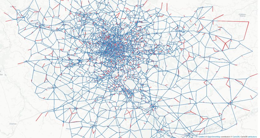
1. Introduction

         Ridesharing, also known as carpooling, is a non-profit shared ride service where a car owner shares his/her
     vehicle with another person heading in the same direction to share expenses. It aims to solve one key problem
     of urban congestion: low vehicle occupancy, especially for commuting trips. In the Paris region, there are 1.05
5    persons per vehicle on average for commuting trips (Enquête Globale Transport, 2010). This rate has been
     decreasing since 1976 (Cornut, 2017). In urban areas, congestion also has severe implications with regards
     to air pollution. Ridesharing offers the opportunity to raise average vehicle occupancy and to address public
     health and climate change issues.
         In this work, we propose a ridesharing scheme quite similar to conventional hitchhiking. Drivers do not
10   deviate from their predetermined itinerary, meaning they determine their optimal departure time and exact
     route without considering a potential rider. The rider than adapts to the itinerary of the matched driver.
     This implies that the rider may need to walk to reach the driver and to reach his/her final destination after
     being dropped off by the driver. However, similar to hitchhiking, the trip is assumed to be completely free
     of charge for the rider.
15       In a more elaborate version, to come, subscribers will be able to travel the various segments of their trip
     on the most appropriate transport mode. For example, a trip might include a walk to a meeting point, a
     ride as a passenger in a personal vehicle, a public transport segment, and another ride as a passenger in
     a personal vehicle to the final destination.3 Here we limit our investigation to three-leg trips: a walk to a
     meeting point, a ride as a passenger in a personal vehicle, and another walk to the final destination. Our
20   key hypothesis is that the segment of the rider’s trip spent in a personal vehicle, will be offered by a driver
     who has already planned to travel that segment on his/her own trip. This is the key feature of our system:
     drivers are inflexible as for hitchhiking. This hypothesis is explained by the observation that one of the
     setbacks in the development of the ridesharing process is that the driver is reluctant to change his/her route
     or his/her scheduling. One cannot avoid the a priori inconvenience to have another person in the car; later
25   on, one can think of some certification systems to reduce the uncertainty to have somebody else (unknown)
     in his/her own car. Of course, such certification (of the car, of the insurance status of the driving license)
     should preserve anonymity and should not be incompatible with privacy rules.
         The 2017 global market size for on-demand transportation was valued at $75 billion and it is expected
     to grow at a 20 % annual rate from 2018 to 2025.4 The impact of COVID-19 increases the attractiveness of
30   private transportation, as was observed in many cities worldwide.
         The emergence of ride-sharing services such as UberPool, Lyft Line, and Blablacar Daily (not to be
     confused with the ride hailing services provided by Uber and Lyft) has been a major competitor to the

        3 In   order to be successful, the system also expects to successfully negotiate with transport providers, whether they are public
     administrations or private entities, to operate on the public right-of-way, to exploit existing on-demand transport networks (such
     as Uber and Lyft), and to access existing public transport services. But again, this discussion has to be postponed for later.
        4 https://www.marketsandmarkets.com/Market-Reports/mobility-on-demand-market-198699113.html

                                                                        2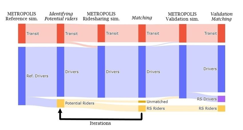
practice of ridesharing (Shaheen and Cohen, 2019). Ridesharing consists of people with similar travel needs
     traveling together, whereas ride hailing consists of car owners offering paid lifts to gain money. The social
35   benefits of ridesharing are manifold: less traffic congestion (Xu et al., 2015; Cici et al., 2014), less CO2 and
     N Ox emissions leading to better air quality (Bruck et al., 2017), and better transit accessibility in suburban
     areas (Teubner and Flath, 2015; Li et al., 2016; Kong et al., 2020). Moreover, ridesharing brings about travel
     cost sharing for riders and drivers (Malichová et al., 2020). However, the popularity of ridesharing remains
     low for commuting trips.
40      Many forms of ridesharing have been studied over the years to increase the mode’s convenience and
     maximise the societal gains it provides in terms of traffic congestion as well as of emissions reduction.
     Nonetheless, each of them presents certain drawbacks. For instance, multi-hop ridesharing explores the
     possibility for a rider to use multiple cars to complete his/her trip at the cost of a transfer penalty and
     waiting time. As for detours created by door-to-door ridesharing services, they increase the driver’s travel
45   distance and time, all the more in the case of multiple passengers. Some ridesharing companies have stopped
     door-to-door service and now ask riders to walk in order to reduce the extent of the detours (Schaller, 2021;
     Lo and Morseman, 2018).
        This research proposes a ridesharing scheme where the driver makes no detour at all and no concession
     on his/her schedule. The rider may therefore need to walk to reach the vehicle and to adapt his/her arrival
50   time to the schedule of the driver (this will not be the case for the on-line reservation system). The only
     difference in the driver’s generalised cost is the inconvenience associated with taking someone in his/her
     car. In order to make ridesharing as attractive as possible, the ride is free of charge for the user and the
     inconvenience of the driver is completely compensated by state subsidies (later on, a monthly/annual public
     transport pass could be required). This study aims to assess the potential of this ridesharing scheme and
55   its impact on congestion reduction by testing it with the mesoscopic dynamic traffic simulator Metropolis
     on the Île-de-France network. The simulator uses data from the 2001 Paris travel survey for the morning
     trip (especially commuting) (Direction Régionale de l’Équipement d’Ile-de-France, 2004; Saifuzzaman et al.,
     2012).
        We wish to contribute to the existing literature on the benefits of ridesharing by analysing its congestion
60   reduction potential, whilst considering dynamic congestion (i.e. congestion depends on the time of the day).
     We also propose a new policy framework to promote ridesharing in large urban areas.
        The remainder of this paper is structured as follows. Section 2 reviews the ridesharing literature and the
     ways it is modelled. Section 3 details the proposed ridesharing scheme, the dynamic traffic simulator, and
     the proposed driver-rider matching methodology. Section 4 presents the case study results for Île-de-France
65   (Paris area) under three maximum walking time scenarios, and for various penetration rates. Section 5
     concludes with the key results and explores further research steps needed to explore the feasibility of a real
     operational-system.

                                                            3
2. Literature Review
Sharing mobility is part of the global trend towards a sharing economy (Standing et al., 2019). Shaheen
70 and Cohen (2019) provide an overview of the different shared-ride services. Ridesharing, also known as
carpooling, and ridehailing, also known as ridesourcing, are two of the main shared-ride services. Whereas
the former is associated with many societal benefits, the latter is an on-demand transportation service
similar to taxi service with privately owned vehicles. Ridehailing is often associated with an increased traffic
congestion (Schaller, 2021). Ridesharing is inherently a non-profit mode that brings together people with
75 similar trip itineraries to share their trip. The body of literature on this topic has significantly increased in
the last decade as it has become more convenient to plan, book, and pay for a ride (Shaheen and Cohen,
2019). Indeed, Transportation Network Companies (TNCs) such as Uber and Lyft offer online ridesharing
services (UberPool and Lyft Line) in addition to their standard ridehailing services.
The matching problem between the rider and the driver has been extensively studied. Matching problems
80 can be either static (Liu et al., 2020; Herbawi and Weber, 2012; Yan and Chen, 2011; Ma et al., 2019a; Lu
et al., 2020) or dynamic (Agatz et al., 2011; Kleiner et al., 2011; Di Febbraro et al., 2013). In static matching
problems, all drivers and riders are known in advance and are matched at the same time. Dynamic matching
problems consider that drivers and riders arrive gradually. In this case, partial matchings can be performed
with a subset of the drivers and riders. This work uses static ridesharing under dynamic congestion.
85 The main benefit of ridesharing is that it eases traffic congestion (Xu et al., 2015; Cici et al., 2014). It
hence offers a great potential for CO2 emission reductions (Bruck et al., 2017; Chan and Shaheen, 2012).
Furthermore, it offers more accessibility to public transit as a first/last mile solution (Teubner and Flath,
2015; Li et al., 2016; Kong et al., 2020). Ridesharing may, however, increase the driver’s trip time through
detours to pick up and drop off riders (Diao et al., 2021). Schaller (2021) analyse extensive longitudinal data
90 from TNCs in American cities. They observe that ridesharing services mainly draw people from transit as
it is mostly popular in neighbourhoods with low incomes and low car ownership rates. This phenomenon
has become even more evident since UberPool and Lyft Line stopped door-to-door services, with the aim
to reduce detours. This finding is in line with many other studies concluding that an increase in the modal
share of ridesharing does not cause a significant reduction in the modal share of car (Kong et al., 2020; Li
95 et al., 2016; Coulombel et al., 2019; Xu et al., 2015; Shaheen et al., 2016). The ridesharing scheme proposed
in this study only allows former drivers to become riders to avoid this rebound effect. Thereby, we consider
a ridesharing scheme, that can be a competitive alternative against private transportation.
Despite the many benefits of ridesharing, it is still not widely used as a mode to commute (Liu et al., 2020).
Amongst the challenges to have a successful ridesharing system is the large population of drivers necessary
100 to provide high-quality matches in terms of geographic and temporal proximity (Bahat and Bekhor, 2016).
Substantial research has been conducted to understand the individual motivations behind ridesharing in
order to increase its popularity. Cost savings followed by environmental concerns are the main motivations
reported both for the drivers and the riders (Neoh et al., 2017; Pinto et al., 2019; Delhomme and Gheorghiu,
42016; Gheorghiu and Delhomme, 2018). Malichová et al. (2020) observed through a pan-European survey
105 that travelers prefer to adopt ridesharing for work compared to other purposes.
Ridesharing has been modelled alongside transit both as a complement providing a solution to the first/last
mile problem (Kumar and Khani, 2020; Reck and Axhausen, 2020; Masoud et al., 2017; Ma et al., 2019b) and
as a competitor (Qian and Zhang, 2011; Galland et al., 2014; Friedrich et al., 2018). Qian and Zhang (2011)
use a theoretical bottleneck model where the modal choice between car, transit, and ridesharing depends on
110 the generalised travel time. They account for transit perceived-inconvenience depending on transit passenger-
flow. Schedule delay is considered for the three modes. de Palma et al. (2020) build on this framework to add
dynamic congestion. Coulombel et al. (2019) use a transportation-integrated land use model to consider the
impact of ridesharing on car and transit ridership for the Paris region. Finally, Galland et al. (2014) propose
an agent-based model for ridesharing to analyse individual mobility behaviour. They test their model on a
115 population of 1000 agents only due to its computational complexity. To predict the route taken by the drivers
in a large-scale scenario, this work uses the dynamic traffic-assignment simulator Metropolis (de Palma
et al., 1997; de Palma and Marchal, 2002). As Metropolis is a dynamic model, we can also account for
the timing of the trips when matching riders with drivers. Metropolis computes, for each individual, the
route, departure-time and mode choice, using a nested Logit model. The schedule-delay costs are based on
120 idiosyncratic α − β − γ preferences (Vickrey, 1969) and congestion is modelled with link-specific bottlenecks.
This work builds on the many ridesharing models present in the literature. The methodology allows to
assess the potential of ridesharing in a large urban area under dynamic congestion, whereas previous models
were either applied on simple bottleneck models (de Palma et al., 2020; Qian and Zhang, 2011; Yu et al.,
2019) or were too sophisticated to provide results for a large urban network (Galland et al., 2014).
125 3. Methodology
3.1. Ridesharing Scheme
This paper explores a ridesharing scheme where ridesharing drivers make no detour and keep the exact
same schedule as when driving alone. Ridesharing drivers simply pick up a passenger at a defined road
intersection on their itinerary and drop off their passenger at another intersection on their itinerary. As
130 for the riders, they need to walk from their origin to a pick-up point and from a drop-off point to their
destination. They face schedule-delay costs if their arrival time does not match their desired arrival time.
However, the trip is free of fare for them.
Figure 1 provides an example of a ridesharing trip under this scheme. The driver itinerary is shown in red
whilst the rider itinerary is in orange. The rider is picked up near his / her origin node (OP ) and dropped off
135 near his / her destination node (DP ). In this example, the rider walks approximately for 100 meters between
his / her origin and the pick-up point (as shown by the grey line).
Implementing such a ridesharing scheme on a large scale would require some sort of state intervention,
in order to convince enough drivers and riders to subscribe to the scheme. We assume in the following
5Figure 1: Ridesharing trip example where OD and DD are the origin and destination of the driver, OP and DP are the origin
and destination of the rider, the red line represents the driver’s trip, the orange line represents the rider’s trip by car and the
grey line represents the rider’s trip by foot.
that subsidies are proposed to the drivers who agreed to pick up someone in their car. These subsidies are
140 deemed small since drivers keep their itinerary and schedule and thus the only cost incurred by them is
the inconvenience of having someone in their car. In practice, the subsidy program could be similar to the
one currently implemented in the Île-de-France region (see details in Section 4), where drivers receive a fix
amount for engaging into ridesharing and an additional subsidy depending on the shared trip length.5
Riders may experience an inconvenience cost, arising from the discomfort of sharing a ride with a stranger
145 (Li et al., 2020). They also have to walk and may incur additional schedule-delay costs. However, the scheme
allows them to save money on gas, car wear and tear, parking, and car insurances. Moreover, they do not
spent time driving around for a parking slot anymore. Still, if the costs of ridesharing are larger than the
benefits, for some individuals, the regulator could propose subsidies to some riders.
An increase in the modal share of ridesharing can greatly reduce the congestion in a city. By increasing
150 the occupancy of vehicles, the number of vehicles on the road decreases. In turn, the externalities associated
with congestion (including air pollution, noise pollution and safety) also decrease. Public authorities may
therefore be interested in subsidizing ridesharing to reduce congestion and its environmental cost. However,
subsidizing ridesharing is only effective if rebound effects (e.g., transit users are getting back to their car) are
limited. To prevent the emergence of rebound effects, three criteria are imposed on the potential riders:
155 1. The scheme only allows riders to use ridesharing for commuting trips. This prevent an increase of the
travel demand because of subsidized trips.
5 https://www.iledefrance.fr/covoiturage-gratuit-lors-des-pics-de-pollution
62. The scheme only allows former drivers to become riders. This prevent transit users from switch to
ridesharing.
3. The scheme only allows riders whose free-flow travel-time between origin and destination is greater
160 than a free-flow travel-time threshold (F F T T threshold ). The free-flow travel-time is the travel time of a
trip when there is no congestion. Switching long car trips to ridesharing saves more vehicle-kilometers
traveled (V KT saved ) than short trips. Encouraging long trips to switch to ridesharing thus provides
more benefits in terms of traffic congestion and pollution reduction.
Although these criteria impede transit users from becoming riders, they do not withhold transit users to get
165 back to their car, as drivers (which they may do if congestion decreases). Typically, as congestion decreases,
some transit users will tend to drive.
3.2. The proposed 6-step Procedure
We do not model explicitly the choice between being a rider or not. Instead, we estimate the maximum
number of acceptable matches between riders and drivers, where riders are selected as a random sample
170 in the population. A match is acceptable if it satisfies some spatial (limited walking time) and temporal
(limited schedule delay) constraints. These constraints and the matching process are detailed in Section 3.5.
Therefore, we provide a lower bound of expected benefits from carpooling, since better matching processes,
based for example on inconvenience costs, can be envisaged.
To find the maximum number of acceptable matches, we run the traffic simulator Metropolis and the
175 matching process with different numbers of riders. Since total travel demand is assumed to be inelastic, the
number of drivers decreases when the number of riders increases. Therefore, as the number of riders increases,
there are less opportunities for good matches and thus the share of riders that can be matched decreases.
To find the maximum number of acceptable matches, we use the following 6-step procedure, illustrated
in Figure 2.
180 1. Metropolis Reference simulation: The traffic simulator Metropolis is run up to a stationary regime,
with all the travel demand. It provides the level of congestion in the scenario with no ridesharing.
Further explanations about the traffic simulator are presented in Section 3.3.
2. Identification of potential riders: Potential riders are randomly chosen among the travelers eligible to
the ridesharing scheme (commuters, former drivers and trip duration ≥ F F T T threshold ).
185 3. Metropolis Ridesharing simulation: Metropolis is run without the selected riders. The removal of
the potential riders creates a new equilibrium with less traffic congestion. The results of the simulation
give the itineraries of the potential ridesharing drivers.
4. Matching: Potential drivers and riders are matched according to the greedy algorithm described in
Section 3.5. Steps 2 to 4 are repeated with different numbers of potential riders to find the highest
190 number of matches.
7Figure 2: Schematic representation of each step performed to assess the potential of the proposed ridesharing (RS) scheme
5. Metropolis Validation simulation: For the number of potential riders that maximizes the number of
matches, some riders are still unmatched. They are put back into the traffic simulator for a validation
simulation, which gives the state of the network when all riders are successfully matched.
6. Validation matching: Previously identified riders are matched with the new set of potential drivers.
195 A small portion of riders cannot be re-matched successfully in the validation matching because the
itineraries and schedules of the drivers change between the Ridesharing simulation and the Validation
simulation. As it was possible to serve all ridesharing requests in the Ridesharing simulation, all requests
are deemed matchable. The results from the validation matching are the ones that are presented in the
results section below.
200 3.3. Traffic Simulator
To assess how congestion evolves as the number of cars decreases and car occupancy increases, we use
Metropolis, a mesoscopic dynamic traffic simulator developed by de Palma et al. (1997). Since then, it has
mostly been used to estimate various transport policies, including different road pricing schemes (Saifuzzaman
et al., 2016; de Palma et al., 2005). Metropolis uses a day-to-day iterative procedure. At each iteration, the
205 travelers choose their mode, departure-time and route, given the expected dynamic congestion levels. At the
end of each iteration (day), the expected congestion levels are updated using the observed congestion levels,
according to a day-to-day adjustment process: the expected congestion for the next iteration is a weighted
average of the current expected congestion and the observed congestion. The simulation stops when the
8two levels are close, i.e., when a stationary equilibrium is reached. The outputs of Metropolis include the
210 itineraries of travelers, the travel costs and the schedule delay costs.
The choices made by each traveler in Metropolis can be summarised as:
1. Mode choice (between car and transit): The generalised cost for transit is compared with the generalised
cost for car. The public transit cost is function of the value of time of transit, the transit travel time,
and the transit fare. In the current version, generalized public transport costs are exogeneous. The
215 generalised cost for car is function of the value of time of car, the endogenous travel-time, and the
schedule-delay cost. The mode choice is given by a nested logit model.
2. Departure-time choice: The probability of choosing a departure time t is given by a continuous logit
model, according to the generalised cost for each possible departure time.
3. Route choice: Each day, at each intersection, travelers observe the congestion on upstream roads and
220 choose a road in order to minimize their generalised cost (closed loop equilibrium).
Note that commuters only choose between car and transit, and ride-sharing is not explicitly modelled as a
mode. By assumption, drivers and riders are always fully compensated for ride-sharing inconvenience, which
justifies their mode choice for ride-sharing if they are matched.
3.4. Ridesharing Cost
225 The cost of ridesharing, for a rider, is the sum of walking cost, in-vehicle cost and schedule-delay cost.
The walking cost is the cost of walking from the origin to the pickup-point and from the drop-off point to the
destination. Let vwalk be the walking speed. The duration of the walking trip from the rider’s origin to the
pick-up point is assumed to be dpick /vwalk , where dpick is the Euclidian distance between the rider’s origin
and the pick-up point. The duration of the walking trip from the drop-off point to the rider’s destination is
230 assumed to be ddrop /vwalk , where ddrop is the Euclidian distance between the drop-off point and the rider’s
destination.
The time at which the driver picks up the rider is denoted tpick and the time at which the driver drops
off the rider is denoted tdrop . Then, the duration of the car trip for the rider is ttiv = tdrop − tpick and the
arrival time at destination is ta = tdrop + ddrop /vwalk .
Each rider has a specific desired arrival time t∗ and a tolerance for lateness or earliness ∆. Riders who
reach their destination within the t∗ ± ∆ window experience no schedule-delay penalty. Every minute outside
this on-time window generates a schedule delay cost. The schedule delay cost of ridesharing is
+ +
SDRS = β (t∗ − ∆) − ta + γ ta − (t∗ + ∆) ,
235 where ta = tdrop + ddrop /vwalk is the arrival time of the rider at destination, β is the penalty associated to
early arrival, γ is the penalty associated to late arrival, and [x]+ = max(0, x).
9To sum up, the generalised cost of ridesharing is
dpick + ddrop
CostRS = αRS · ttiv + αwalk · + SDRS ,
| {z } vwalk | {z }
In-vehicle cost | {z } Schedule-delay cost
Walking cost
where αRS is the value of time of riders during the ride and αwalk is the value of time of walking. Note that
the waiting time of the rider at the pick-up point is neglected.
3.5. Matching
240 The off-line matching of riders with drivers is assumed to be managed by a single operator who is assumed
to be fully informed with regards to trips, costs, and user preferences. It is assumed to take place before any
departure.
To simplify, we assume that each driver picks up at most one rider in his/her car. We also impose that all
matches satisfy a spatial and temporal constraint. The spatial constraint ensures that the walking distance
245 from origin and to destination is not larger than dmax , i.e., we only consider potential matches for which
dpick ≤ dmax and ddrop ≤ dmax . The temporal constraint ensures that the rider does not arrive too early or
too late at his / her destination, i.e., we only consider potential matches for which the arrival time at the
drop-off point is such that tdrop ∈ [ t∗rider − δe , t∗rider + δl ].
Not all drivers are willing to share a ride, even if they receive compensation for it. The reason might
250 be that they are driving their kids to school or that their car is full of shopping items. To represent these
drivers, we remove a fixed percentage of vehicles from the matching process.
We use a greedy heuristic method aimed at minimising the total ridesharing generalised cost. The
matching between the set of potential drivers and the set of potential riders is a two-step process:
1. For each rider request, potential matches that follow the spatial and temporal constraints are identified
255 and the generalised cost of each match is computed. If a vehicle offers multiple trip alternatives to a
rider (i.e., multiple pick-up/drop-off points satisfy the constraints), the trip with the smallest cost is
kept for the following step. An example of the result of this step is presented in Table 1a.
2. All the potential matches are sorted by the sum of the walking and schedule delay cost (denoted as
Cost in Table 1). The in-vehicle cost is excluded as it would result in matching short trips first. Riders
260 and drivers are then matched following a greedy algorithm. Tables 1b, 1c and 1d display an example of
greedy matching for three riders. The match with the lowest cost at each step is identified and added
to a list of confirmed matches. Once a vehicle is matched, all potential trips associated with this vehicle
are removed from the list of potential trips. In addition, once a rider’s request is served, all other trips
proposed to this rider are removed from the list of potential trips.
265 Note that, if the spatial and temporal constraints are too restrictive, some riders might not be matched to any
driver. In this case, the unmatched rider is unable to participate in the ridesharing program and therefore
uses an alternative mode of transport.
10Rider ID Driver ID Cost
1 12 0
1 13 0.2
1 14 0.5
2 12 0.4
2 15 1.1
2 16 1.3
3 13 0.7
3 15 2.4
(a) All possible trips
Rider ID Driver ID Cost
1 12 0 Rider ID Driver ID Cost
Rider ID Driver ID Cost
1 13 0.2
1 12 0
2 12 0.4 1 12 0
3 13 0.7
1 14 0.5 3 13 0.7
2 15 1.1
3 13 0.7 2 15 1.1
2 16 1.3
2 15 1.1 2 16 1.3
3 15 2.4
2 16 1.3
(d) Match 3
3 15 2.4 (c) Match 2
(b) Match 1
Table 1: Matching process between the drivers and the riders
Note. The green rows represent the confirmed matches. The gray rows represent the matches no longer available because
either the rider or the driver is already matched.
114. Case Study: Ridesharing in Île-de-France
The Paris area, as many other large cities, experiences frequent heavy pollution episodes partly due to
270 car emissions (Kumar et al., 2021; Degraeuwe et al., 2017). The regional government of Île-de-France created
subsidy programs in 2017 to promote ridesharing and address this issue. The programs include, inter alia,
direct subsidies for ridesharing drivers, the funding of ridesharing companies so that they offer lower fares to
riders, and two monthly free rides to frequent transit users. Drivers receive from the government 1.50 e per
passenger plus 0.10 e/km up until a maximum of 3 e per trip. Moreover, the regional government has made
275 ridesharing completely free for riders during peak pollution episodes and during transit strikes.6 7
The ridesharing scheme proposed in this research is tested on the Île-de-France region. Île-de-France
accounts for nearly a fifth of France’s population with its 12 175 000 inhabitants in 2017. The region, mainly
consisting of Paris and its suburbs, has a density of 1013 inhabitants per squared kilometer. Regionwide,
there are 43 million trips daily amongst which 42 % are made by foot or bicycle, 22 % by public transit, and
280 36 % by car. There are however wide disparities between the city of Paris, the inner and the outer suburbs
(Île-de-France Mobilités, 2019).
4.1. Network Modelling
We use the calibration of Metropolis for Île-de-France from Saifuzzaman et al. (2012), which is based on
demand data from the 2001 Paris origin-destination survey. The road network consists of 43 857 links, 18 584
285 intersections, and 1360 zones. Each link is unidirectional and represents a bottleneck with a link-specific
capacity. The origin and destination of travelers is set to the centroid of their origin / destination zone. The
centroids are connected to the road network with uncongested links. Figure 3 is a visual representation of the
network. Compared to the original calibration by Saifuzzaman et al. (2012), we enable mode choice, which
requires recalibrating the road capacities.
290 There is no public transit network per se, but rather exogenous travel times for each origin and destination
pair of Île-de-France. The public-transit generalized costs are taken from the DRIEAT (Direction régionale
et interdépartementale de l’environnement, de l’aménagement et des transports d’Île-de-France).
The computed walking distance is the euclidean distance between the centroid of the zones and the
intersections. Note that, some centroids are too far from the road network to allow the rider to walk under
295 the spatial constraint, i.e., they can only take drivers who have the same origin or destination. For instance,
21 % of the 1360 zones are at more than 500 meters of any road intersection, and 10 % are at more than
1000 meters.
6 https://www.iledefrance.fr/la-prime-au-covoiturage-prolongee-et-etendue
7 https://www.iledefrance.fr/covoiturage-jusqua-150-euros-par-mois-pour-les-conducteurs
12Figure 3: Île-de-France road network
Note. Red lines are uncongested roads connecting the centroids of the zones to the road network (in blue).
4.2. Travel Demand
We simulate the morning commute, which is the most congested period of the day in Île-de-France.
300 The simulation starts at 6AM and ends at 12PM. Travel demand is represented in Metropolis as an
origin-destination matrix for different traveler groups. All demand data are taken from the calibration of
Metropolis for Île-de-France (Saifuzzaman et al., 2012). Travel demand for the morning commute is divided
in four traveler groups: workers going towards Paris, workers leaving Paris, and two groups of non-workers.
Both the demand and the road capacity are scaled-down to reduce computation time. There is a total of
305 934 042 travelers.
In each group, the travelers have the same schedule-delay parameters and values of time but the desired
arrival times are normally distributed. Figure 4 represents the desired arrival time distribution for the four
groups of travelers. Workers coming from Paris are the ones with the narrowest distribution and the earliest
desired arrival time. The workers originating from the suburbs and going towards Paris want to reach their
310 destination, in average, a few minutes later. The desired arrival time of the non-workers is represented by
two normal curves with a standard-deviation of 90 minutes. Non-workers have a later desired arrival time
than commuters.
In Metropolis, the driver’s on-time window is centered around the desired arrival time t∗driver and
has a length of 2∆, where ∆ represents the acceptable lateness or earliness (i.e., without penalty). It
315 is is fixed at ∆ = 5 min and identical for all traveler groups. Although this hypothesis is valid for a
mesoscopic analysis, it fails to represent the greater flexibility some individuals, such as office workers, have
in their desired arrival time window. A rider-specific delay tolerance is drawn from the lognormal distribution
∆ ∼ Lognormal(2, 1)+3 min to replace the constant value of five minutes for matched riders. This distribution
131RQ ZRUNHUV
1RQ ZRUNHUV
:RUNHUV OHDYLQJ 3DULV
:RUNHUV JRLQJ WRZDUGV 3DULV
3UREDELOLW\ 'HQVLW\
'HVLUHG DUULYDO WLPH W KRXU
Figure 4: Desired arrival time distribution of the four traveler groups
also reflects the fact that some riders are ready to arrive earlier or later at work in order to find a ridesharing
320 match.
All the preference parameters used in this research are presented in Table 2. The values of time for car
and transit as well as the early and late penalties come from the work of Saifuzzaman et al. (2012). The value
of time for riders is assumed to be equal to the value of time of car (i.e., αcar = αRS ), which means that for
riders the savings incurred by ridesharing are completely offset by its inconvenience. Workers starting their
325 journey in Paris are more inflexible in their desired arrival time as shown by their penalty for late arrival
being more than twice the one of workers starting their journey in the suburbs. The value of time of walking
is assumed to be αwalk = 1.1 · αRS . This hypothesis implies that riders prefer to stay in a car rather than
walk (Hensher and Rose, 2007; Wardman, 2001).
Traveler group β γ αcar αRS αPT αWalk
Workers going towards Paris 6.09 7.53
12.96 12.96 13.24 14.26
Workers coming from Paris 8.36 17.43
Table 2: Preference parameters for the two groups of workers, in e/h
The walking speed is set to 4 km/h. We consider three different scenarii, corresponding to three different
330 values of the maximum walking distance parameter dmax : a door-to-door service scenario (dmax = 0), a
maximum walking time of 15 min per leg of the trip (dmax = 500 m), and a maximum walking time of
30 min per leg of the trip (dmax = 1000 m). The long trip criterion for the riders’ selection is defined as
F F T T threshold = 10 min. This threshold keeps 40 % of the commuting trips. The maximum acceptable
earliness at the drop-off intersection for the rider is set to δe = 60 min, whereas the maximum acceptable
335 lateness is set to δl = 45 min. These parameters are asymmetrical to account for the lower penalty incurred by
early arrival compared to late arrival. Any potential match whose drop-off time is outside the time-window
[t∗rider − 60 min, t∗rider + 45 min] will therefore be ignored. Finally, the share of drivers willing to propose
14Scenario Reference Door-to-door 15 min 30 min
walking time walking time
Congestion 21.7 % 15.1 % 13.9 % 9.29 %
Car VKT (106 km) 10.84 9.69 9.50 8.60
Mean travel cost for drivers (e) 3.29 3.02 2.98 2.76
Mean free-flow travel cost for drivers (e) 2.74 2.60 2.60 2.50
Transit modal share 25.2 % 23.6 % 23.3 % 22.1 %
Car modal share 74.8 % 70.4 % 68.9 % 64.8 %
Ridesharing modal share — 5.9 % 7.8 % 13.1 %
Number of transit users 235 544 221 739 217 591 206 841
Number of drivers 698 499 657 541 643 992 605 093
Number of ridesharing riders — 54 763 72 460 122 109
Table 3: Comparison of results for the reference scenario and three scenarii with different maximum walking time
their car for ridesharing is set at 90 %. This high proportion is used to assess the maximum potential of the
ridesharing scheme. A sensitivity analysis is conducted for this parameter for lower and more realistic values.
340 4.3. Results
Table 3 presents the results from the Metropolis validation simulation for the reference scenario (with
no ridesharing), and the three ridesharing scenarii. The average congestion during the morning commute is
given by
1 X ttavg − tt0l
l
· ,
|L|
l∈L
tt0l
where L is the set of all links in the network, |L| is its cardinality, ttavg
l is the average travel-time on link l
for the recording period and tt0l is the free-flow travel-time of link l. The Car VKT indicator represents the
total distance (in million of kilometers) travelled by cars during the morning commute.
The number of riders chosen in the three ridesharing scenarii is the maximum number of matches respect-
345 ing the temporal and spatial constraints, i.e., as the number of riders increase beyond this point, the number
of available drivers is so low that not all riders can be matched, under the temporal and spatial constraints.
Under the door-to-door scenario the modal share of ridesharing riders is 5.9 %. In this scenario, the driver
and the rider must share the same origin zone and destination zone. It brings road congestion from 21.7 %
to 15.1 % with 54 763 ridesharing trips. Schedule delay and travel costs are reduced for all road users as a
350 consequence of lower road congestion. The free-flow travel-cost also improves as less detours are made to
avoid congested areas.
By considering that riders can walk from their origin to a pick-up intersection and from a drop-off
intersection to their destination, the maximum number of requests that can be matched increases together
15with the ridesharing modal share and benefits. The main drawback of an increased ridesharing modal share
355 is a larger shift from public transit to car. Yet the shift is contained as only former drivers are eligible to
take part in the ridesharing scheme. The modal shift is attributable to the increased attractiveness of car
compared to transit under lower congestion. Indeed, by removing vehicles from the road network, congestion
decreases and the generalised cost of driving decreases. The generalised cost of transit stays identical since it
is exogenous and independent from congestion in Metropolis. For the 15-minute maximum walk scenario
360 only 1.9 % of travelers are transit users who shifted to solo driving, while 7.8 % of travelers are riders.
The percentage of drivers willing to participate in the program is the only constraint restraining the set of
potential drivers. It is set at 90 % for all results presented. This share assesses a maximum potential. Figure
5 presents the ridesharing share and the level of congestion as a function of the percentage of drivers willing to
participate in the ridesharing scheme for the 15-minute maximum walking time scenario. It can be observed
365 that with only 10 % of drivers willing to participate (randomly distributed across the Île-de-France region),
the ridesharing share is smaller than 2 % and thus the congestion reduction is insignificant the number of
ridesharing matches and hence the congestion reduction is insignificant. With half the drivers willing to
engage in the ridesharing scheme, the ridesharing share goes up to about 5.5 %, inducing a congestion level
only slightly larger than with 90 % of potential drivers (15.5 % versus 13.9 %). Complete results are presented
370 in Appendix B for 20 % of drivers willing to participate in the program.
10% 25%
8% 20%
Ridesharing share
Congestion level
6% 15%
4% 10%
2% 5%
0% 0%
0% 20% 40% 60% 80% 100%
Percentage of vehicles willing to participate in the ridesharing scheme
Figure 5: Sensitivity analysis of the percentage of drivers willing to participate in the ridesharing scheme for the 15-minute
walking time scenario.
The travel survey used for the Île-de-France model (EGT 2001, Direction Régionale de l’Équipement
d’Ile-de-France, 2004) has 2.93 million commuting trips (car + transit) for the morning commute, whereas
the OD matrices in Metropolis are scaled down to a total of 513 549 commuting trips. Some results,
including Car VKT and the number of riders, need to be rescaled to be meaningful. The traffic simulator
375 gives identical results as long as the demand (OD matrices) and the supply (road network) are scaled down
16in the same proportion. But, more travelers in the matching model means more ridesharing opportunities
as the probability of finding multiple vehicles answering a ridesharing request increases. The same request
might then be served with less schedule delay and walking time. The rescaled results therefore probably
underestimate the potential of ridesharing matches. The rescaled results are presented in Table 4 alongside
380 travel time savings and carbon dioxide equivalent emission savings.
Scenario Reference Door-to-door 15 min 30 min
walking time walking time
Rescaled Car VKT (106 km) 61.7 55.2 54.1 49.0
Fuel savings (L) - 526 000 611 000 1 023 000
CO2eq emission avoided (tons) - 1270 1474 2467
CO2eq emission avoided (%) - 10.5 % 12.3 % 20.6 %
Travel-time savings (h) - 97 900 106 000 160 000
Travel-time savings (%) - 10.1 % 11.1 % 17.9 %
Number of ridesharing riders - 311 911 412 707 695 491
Number of drivers 3 981 494 3 747 984 3 670 754 3 449 030
Travel-time savings per road user (min) - 1.57 1.73 2.78
Table 4: Rescaled results and savings for the reference scenario and three scenarii with different maximum walking time
Note. Average fuel consumption: 8 L/100 km (Agence de la transition écologique, 2018). Average car CO2eq emissions:
0.193 kg of CO2eq / km (Agence de la transition écologique, 2021)
With near four million travelers during the morning commute, the benefits of ridesharing are significant.
The 30-minute maximum walking time scenario brings a decrease of about 21 % in Car VKT and carbon
dioxide equivalent (CO2eq ) emissions, compared to the reference scenario. The savings are halved in the
door-to-door scenario. At an individual level, road users save on average 1.73 minutes of travel time during
385 the morning commute under the 15-minute scenario. The travel time savings amount to 106 000 hours
network-wide under the same scenario. The travel time savings of riders are analysed further in Figure 11.
4.4. Detailed Results for the 15-minute Maximum Walking Time Scenario
The scenario with a maximum walking time of 15 minutes offers a good improvement in road congestion
at a relatively low walking cost for the riders. When 90 % of vehicles are willing to engage into the program,
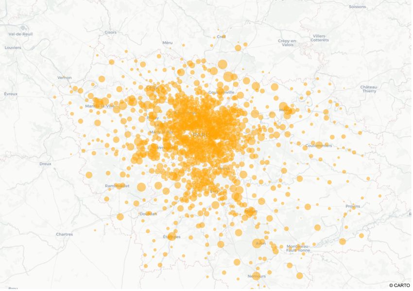
390 ridesharing opportunities arise everywhere in Île-de-France, even in rural areas. Figure 6 presents the origins
and destinations of all matched riders. The most frequent origins and destinations are the same as in the
overall population. In that respect, the two main destinations are the two largest economic hubs: Paris’ CBD
(La Défense) and Paris Charles-de-Gaulle Airport (Roissypôle). In contrast, the origins are scattered across
the greater Paris area.
17(a) Riders’ origins (b) Riders’ destinations
Figure 6: Origins and destinations of matched riders in Île-de-France
395 In this scenario, there are 72 460 ridesharing trips. Figure 7 represents the distribution of the riding times,
i.e., the in-vehicle travel time of riders between the pick-up and the drop-off intersections. The mean riding
time is 18 minutes. This is higher than the mean driving time of 14 minutes observed amongst ridesharing
and non-ridesharing drivers. The discrepancy is explained by the fact that the ridesharing scheme is only
accessible to travelers who used to commute by car, with a trip longer than 10 minutes of free-flow travel-
400 time. In fact, if we only consider the ridesharing and non-ridesharing drivers with a free-flow travel-time of
10 minutes, we get an average travel-time of 24 minutes. Observe that, for 10 % of riders, the riding time is
smaller than 10 minutes, even though their free-flow travel-time was larger than 10 minutes when driving.
The reason is that, as congestion decreases, some vehicles offering a ridesharing trip may take a shorter
itinerary than the one that was taken by the rider when he/she was driving.
3HUFHQWDJH
5LGH WLPH PLQXWHV
Figure 7: Distribution of riding time for the matched riders
405 The total walking distance displayed on Figure 8 represents the sum of the euclidean distances between the
rider’s origin zone and the pick-up intersection (maximum 500 meters) and between the drop-off intersection
and the rider’s destination zone (maximum 500 meters). The maximum walking distance is therefore 1km in
this scenario. There is no walking at all for 56 % of matches, meaning that the rider and the driver have the
same OD pair. This data is not displayed on the figure to facilitate its reading. The large gap observed at 500
18410 meters is explained by the fact that most riders walk only at one end of their trip chain. In fact, only 5 % of
riders walk at both ends. Even though the maximum walking time for one leg of the trip is 7.5 minutes, only
3 % of riders walk for more than that time for the whole trip. The mean walking distance in this scenario is
141 meters, which corresponds to a mean walking cost of 0.50 e. By allowing a maximum 15-minute walk,
the modal share of ridesharing improves by 1.9 % compared to the door-to-door scenario only at the cost of
415 a small walking time for riders.
3HUFHQWDJH
7RWDO ZDONLQJ GLVWDQFH P
Figure 8: Distribution of walking distance for the matched riders
Note. The 56 % of riders with a null walking distance are excluded from the graph.
Figure 9 presents the schedule delay of riders for the lognormal and constant values of ∆. Schedule delay
occurs when a traveler arrives at destination outside the desired arrival time window. The remainder of
this analysis only considers the lognormal distribution of delay tolerance. The figure excludes riders whose
schedule delay is null (59 % of all riders) to clarify the presentation. The mean delay is 14 minutes for early
420 arrivals and 11 minutes for late arrivals. Together, they represent a mean schedule delay cost of 0.80 e.
'HOD\ WROHUDQFH
/RJQRUPDO
PLQXWHV
3HUFHQWDJH
í í í í í í
6FKHGXOH 'HOD\ PLQXWHV
Figure 9: Distribution of schedule delay for the matched riders
Note. The 59 % of riders experiencing no schedule delay are excluded from the graph.
Complete statistics for riding time, walking distance and schedule delay are presented in Appendix A.
Figure 10 presents the distribution of the generalised cost of ridesharing for riders. It is the sum of the
schedule delay cost, the walking cost, and the in-vehicle travel cost. An analysis of the ridesharing cost
reveals that the main component is the in-vehicle travel cost: the mean cost of 5.09 e can be divided in 16 %
193HUFHQWDJH
5LGHVKDULQJ JHQHUDOLVHG FRVW (XURV
Figure 10: Distribution of the riders’ generalised ridesharing cost
425 of schedule delay cost, 10 % of walking cost, and 74 % of in-vehicle travel cost.
3HUFHQWDJH
3HUFHQWDJH
í í í í í í
5LGLQJ WLPH JDLQ PLQXWHV 7UDYHO WLPH JDLQ PLQXWHV
(a) Riding time gain distribution (ttCar − ttRS ) (b) Travel time gain distribution (ttCar − ttRS − tW )
Figure 11: Riding time and travel time gains of riders, compared to the reference scenario
A comparison of the total travel time and the riding time from an individual point of view allows to better
understand the benefits of ridesharing from the user’s perspective. Figure 11a presents the distribution of
the riding time gain and Figure 11b presents the distribution of the total travel time gain (walking time plus
riding time), for riders, compared to the reference scenario where they used their car. Amongst matched
430 riders, some experience a travel time gain due to lower congestion and a smaller riding time, whilst some
experience a longer travel time caused by a long walking distance. There is a mean riding time gain of 4
minutes and a median riding time gain of 1.8 minutes mainly attributable to the fact that there are less
vehicles on the road network hence making the average travel time 9 % cheaper. However, the travel time
gain shrinks because of the walking cost. The mean travel time gain is 2 minutes and the median travel time
435 gain is only 0.4 minutes. In that respect, 43 % of riders will experience a higher travel time when ridesharing
instead of driving. As stated before, many other factors may encourage ridesharing behaviours, thus making
travelers accept a ridesharing trip with a longer travel time than for car. For example, riders do not need
to search for a parking space and to pay parking costs. On top of this, there is the cost of fuel as well as
psychological factors that can influence their decisions. Riders whose travel time increase is still too large to
440 be acceptable would receive state subsidies to offset it.
205. Conclusion
Carpooling is a tool with a great potential to reduce pollution and congestion in urban areas. It never-
theless remains unpopular amongst commuters, despite a growing number of carpooling apps (i.e. mobile
applications). In this paper, we focus on work commutes because they usually have time-restrictions at the
445 workplace, but there is no need to stick to work related commute in a real-world application. A carpooling
app is definitely needed to make such scheme acceptable. Many other technical problems remain to be solved,
and in particular the driver should have safe and easy to find meeting points to pick-up their passenger.
This study proposes a state-subsidised carpooling scheme to increase the modal share of carpooling. The
potentials of this scheme are tested on the Île-de-France region to evaluate the individual and social benefits.
450 It is based on the dynamic traffic simulator Metropolis and a greedy matching procedure. Drivers and
riders are matched based on their itineraries. We focus on former car drivers who accept to carpool, but
other configuration may be worthwhile exploring: for example, when public transport exists but is of poor
quality.
The carpooling scheme we propose considers, since no detour nor extra schedule delays are involved, that
455 the vast majority of drivers would be ready to pick up someone in their car in exchange for a small monetary
incentive. This state subsidy then only compensates for the inconvenience cost of sharing a car. Riders need
to walk, but benefit from a free ride. Their individual savings are gasoline saving, time and monetary saving
related to parking, and wear and tear (beside the reduced congestion). The social saving is a result of less
vehicles on the road, which means less travel time and therefore less accidents and pollution.
460 Three main scenarios were tested for Île-de-France to show the potential benefits of carpooling. The less
optimistic one (the one where the rider walks in average 141m, and no more than 15 minutes, the maximum
walking time) proves to be also the most interesting one. It saves 7.6 million vehicle-kilometres travelled
for the morning commute, reducing CO2 emissions by 1 474 tons, and travel times by 106 000 hours. This
represents an average time saving of 1.73 minutes per road user.
465 In this paper, we consider the morning commute, which has to be seen as an intermediary step for two
reasons. First, the evening commute is a not a mirror case of the morning commute in dynamic models (as
shown for example by de Palma and Lindsey, 2002). Second, if a user decides not to take his/her car the
morning, he/she has to carpool or take public transport in the evening. Moreover, if the schedule preferences
of two matched users are similar in the morning, this does not necessarily mean they will be similar in the
470 evening for the same driver/rider couple. So, in general, the same match could not be arranged in the morning
and in the evening. As a consequence, the riders are not guaranteed to find another convenient match for
their return trip in the evening. Matching for round-trip commuting is a constraint that could be imposed
on future research. A mathematical formulation of this problem was proposed by de Palma and Nesterov
(2006), in the case of stable-dynamic models.
475 To keep the analysis simple, this research only considered that riders take one car to complete their trip
and that each vehicle can only satisfy one ridesharing request. Allowing for riders to take multiple vehicles
21to satisfy their ridesharing request and for drivers to serve multiple ridesharing requestions can increase
the potential of ridesharing. The success of carpooling depends heavily on how many drivers are willing to
participate. This type of ridesharing, referred to as multi-hop ridesharing, has been recently investigated
480 (Herbawi and Weber, 2012; Teubner and Flath, 2015). Even though multi-hop ridesharing generates transfer
penalties between cars, it could be interesting for some segments of a network, in particular for OD pairs
with low demand. The combinatorial issues (the multiple matching problem) remain widely unexplored in
the matching literature in economics (labour market and marriage market, for rather obvious reasons).
However, it remains to be seen if riders and drivers are prepared to be involved in a more complex
485 organization. Empirical research is needed in order to evaluate the acceptance of such an organization.
Thereby, a mobile application needs to be developed such that all unnecessary complexity is eliminated. For
example, in Uber all the complexity is hidden from drivers and riders.
Another important extension that could be considered is to include an explicit and structural mode choice
model at the individual level. Instead of randomly selecting a fixed number of individuals to be riders, as we
490 did, the mode choice model could be augmented with an endogenous choice to be a rider or not. Moreover,
adding inconvenience cost to match a specific rider with a specific driver will change the results. The
mathematical treatment of this case is rather straightforward, but the empirical required input parameters
are delicate. This would increase the quality of the matches, as the individuals choosing to be riders would be
the ones who can get the highest quality matches (as far as detour, scheduling and idiosyncratic inconvenience
495 costs). This would also allow to better evaluate the subsidies required to convince more drivers to switch to
carpooling.
Acknowledgements
The authors are grateful to Jesse Jacobson for his comments and several discussions. We would also like
to thank Catherine Morency, Nikolas Geroliminis and the participants of the CY economics seminar.
500 Funding
This research did not receive any specific grant from funding agencies in the public, commercial, or
not-for-profit sectors.
References
Agatz, N.A.H., Erera, A.L., Savelsbergh, M.W.P., Wang, X., 2011. Dynamic ride-sharing: A simulation
505 study in metro Atlanta. Transportation Research Part B: Methodological 45, 1450–1464. doi:10.1016/j.
trb.2011.05.017.
Agence de la transition écologique, 2018. Consommations conventionnelles de carburant et émissions de CO2.
Technical Report. ADEME. Paris.
22Agence de la transition écologique, 2021. ADEME - Bilans GES. https://www.bilans-ges.ademe.fr/fr/accueil.
510 Bahat, O., Bekhor, S., 2016. Incorporating Ridesharing in the Static Traffic Assignment Model. Networks
and Spatial Economics 16, 1125–1149. doi:10.1007/s11067-015-9313-7.
Bruck, B.P., Incerti, V., Iori, M., Vignoli, M., 2017. Minimizing CO2 emissions in a practical daily carpooling
problem. Computers & Operations Research 81, 40–50. doi:10.1016/j.cor.2016.12.003.
Chan, N.D., Shaheen, S.A., 2012. Ridesharing in North America: Past, Present, and Future. Transport
515 Reviews 32, 93–112. doi:10.1080/01441647.2011.621557.
Cici, B., Markopoulou, A., Frias-Martinez, E., Laoutaris, N., 2014. Assessing the potential of ride-sharing
using mobile and social data: A tale of four cities, in: Proceedings of the 2014 ACM International Joint
Conference on Pervasive and Ubiquitous Computing, New York, NY, USA. pp. 201–211. doi:10.1145/
2632048.2632055.
520 Cornut, B., 2017. Le Peak Car En Ile-de-France : Etude de l’évolution de La Place de l’automobile et de Ses
Déterminants Chez Les Franciliens Depuis Les Années 1970. Theses. Université Paris-Est.
Coulombel, N., Boutueil, V., Liu, L., Viguié, V., Yin, B., 2019. Substantial rebound effects in urban
ridesharing: Simulating travel decisions in Paris, France. Transportation Research Part D: Transport and
Environment 71, 110–126. doi:10.1016/j.trd.2018.12.006.
525 de Palma, A., Kilani, M., Lindsey, R., 2005. Congestion pricing on a road network: A study using the
dynamic equilibrium simulator METROPOLIS. Transportation Research Part A: Policy and Practice 39,
588–611. doi:10.1016/j.tra.2005.02.018.
de Palma, A., Marchal, F., 2002. Real cases applications of the fully dynamic metropolis tool-box: An
advocacy for large-scale mesoscopic transportation systems. Networks and Spatial Economics 2, 347–369.
530 doi:10.1023/A:1020847511499.
de Palma, A., Marchal, F., Nesterov, Y., 1997. METROPOLIS: Modular System for Dynamic Traffic Simu-
lation. Transportation Research Record 1607, 178–184. doi:10.3141/1607-24.
de Palma, A., Stokkink, P., Geroliminis, N., 2020. Influence of Dynamic Congestion on Carpooling Matching.
Working Paper. THEMA (THéorie Economique, Modélisation et Applications), CY Cergy Paris University.
535 Degraeuwe, B., Thunis, P., Clappier, A., Weiss, M., Lefebvre, W., Janssen, S., Vranckx, S., 2017. Im-
pact of passenger car NOX emissions on urban NO2 pollution – Scenario analysis for 8 European cities.
Atmospheric Environment 171, 330–337. doi:10.1016/j.atmosenv.2017.10.040.
Delhomme, P., Gheorghiu, A., 2016. Comparing French carpoolers and non-carpoolers: Which factors con-
tribute the most to carpooling? Transportation Research Part D: Transport and Environment 42, 1–15.
540 doi:10.1016/j.trd.2015.10.014.
23You can also read