The SOUL view of IRAS 20126+4104 - Kinematics and variability of the H2 jet from a massive protostar - arXiv
←
→
Page content transcription
If your browser does not render page correctly, please read the page content below
Astronomy & Astrophysics manuscript no. iras20126_axv                                                                               ©ESO 2023
                                               January 18, 2023

                                                                                The SOUL view of IRAS 20126+4104.
                                                              Kinematics and variability of the H2 jet from a massive protostar
                                               F. Massi1 , A. Caratti o Garatti2, 3 , R. Cesaroni1 , T. K. Sridharan4, 5 , E. Ghose1 , E. Pinna1 , M. T. Beltrán1 , S. Leurini6 , L.
                                               Moscadelli1 , A. Sanna6 , G. Agapito1 , R. Briguglio1 , J. Christou7 , S. Esposito1 , T. Mazzoni1 , D. Miller7 , C. Plantet1 , J.
                                                                        Power7 , A. Puglisi1 , F. Rossi1 , B. Rothberg7, 8 , G. Taylor7 , and C. Veillet7

                                                     1
                                                         INAF-Osservatorio Astrofisico di Arcetri, Largo E. Fermi 5, I-50125 Firenze, Italy
                                                         e-mail: fabrizio.massi@inaf.it
                                                     2
                                                         INAF-Osservatorio Astronomico di Capodimonte, via Moiariello 16, I-80131 Napoli, Italy
arXiv:2301.06832v1 [astro-ph.SR] 17 Jan 2023

                                                         e-mail: alessio.caratti@inaf.it
                                                     3
                                                         Dublin Institute for Advanced Studies, School of Cosmic Physics, Astronomy and Astrophysics Section, 31 Fitzwilliam Place,
                                                         Dublin 2, Ireland
                                                     4
                                                         National Radio Astronomy Observatory, 520 Edgemont Road, Charlottesville, VA 22903, USA
                                                     5
                                                         Harvard-Smithsonian Center for Astrophysics, 60 Garden Street, Cambridge, MA 02138, USA
                                                     6
                                                         INAF-Osservatorio Astronomico di Cagliari, Via della Scienza 5, I-09047 Selargius (CA), Italy
                                                     7
                                                         Large Binocular Telescope Observatory, 933 N. Cherry Ave #552, Tucson, AZ 85721, USA
                                                     8
                                                         George Mason University, Department of Physics & Astronomy, MS 3F3, 4400 University Dr., Fairfax, VA 22030, USA

                                                    Received ; accepted

                                                                                                                 ABSTRACT

                                                    Context. We exploit the increased sensitivity of the recently installed adaptive optics SOUL at the LBT to obtain new high-spatial-
                                                    resolution near-infrared images of the massive young stellar object IRAS20126+4104 and its outflow.
                                                    Aims. We aim to derive the jet proper motions and kinematics, as well as to study its photometric variability by combining the novel
                                                    performances of SOUL together with previous near-infrared images.
                                                    Methods. We used both broad-band (K s , K 0 ) and narrow-band (Brγ, H2) observations from a number of near-infrared cameras
                                                    (UKIRT/UFTI, SUBARU/CIAO, TNG/NICS, LBT/PISCES, and LBT/LUCI1) to derive maps of the continuum and the H2 emission in
                                                    the 2.12 µm line. Three sets of images, obtained with adaptive optics (AO) systems (CIAO, in 2003; FLAO, in 2012; SOUL, in 2020),
                                                    allowed us to derive the proper motions of a large number of H2 knots along the jet. Photometry from all images was used to study the
                                                    jet variability.
                                                    Results. We derived knot proper motions in the range of 1.7–20.3 mas yr−1 (i.e. 13–158 km s−1 at 1.64 kpc), implying an average
                                                    outflow tangential velocity of ∼ 80 km s−1 . The derived knot dynamical age spans a ∼ 200–4000 yr interval. A ring-like H2 feature near
                                                    the protostar location exhibits peculiar kinematics and may represent the outcome of a wide-angle wind impinging on the outflow
                                                    cavity. Both H2 geometry and velocities agree with those inferred from proper motions of the H2 O masers, located at a smaller distance
                                                    from the protostar. Although the total H2 line emission from the knots does not exhibit time variations at a e  >0.3 mag level, we have
                                                    found a clear continuum flux variation (radiation scattered by the dust in the cavity opened by the jet) which is anti-correlated between
                                                    the blue-shifted and red-shifted lobes and may be periodic (with a period of ∼ 12 − 18 yr). We suggest that the continuum variability
                                                    might be related to inner-disc oscillations which have also caused the jet precession.
                                                    Key words. Stars: formation – ISM: jets and outflows – ISM: individual objects: IRAS20126+4104 – Instrumentation: adaptive
                                                    optics – Infrared: ISM

                                               1. Introduction                                                      tion, namely protostars grow through short episodes of intense
                                                                                                                    matter inflows. If accretion and outflows are linked together, this
                                                                                                                    would in fact agree with the morphology of many optical and
                                               Collimated jets and outflows from low-mass young stars and near-infrared (NIR) jets that appear composed of aligned knots
                                               protostars are ubiquitous and are now believed to be intimately (emitting in several optical and NIR spectral lines), which, in this
                                               linked with accretion discs. The most widely accepted paradigm view, would be relics of past accretion bursts. In this scenario,
                                               is that they originate from magnetically collimated disc winds and both protostars and very young stars should also exhibit photo-
                                               help remove angular momentum from the disc, allowing the gas metric variability with augmented luminosity occurring during
                                               to accrete onto the star surface (see, e. g. Ray & Ferreira 2021 and phases of intense accretion, which has actually been observed
                                               references therein). Another well-established observational fact in both low-mass (see, e. g. Yoo et al. 2017; Caratti o Garatti
                                               in low-mass star formation is the so-called Luminosity Problem, & Eislöffel 2019), intermediate-mass (Benisty et al. 2010) and
                                               whereby protostars are usually much fainter than predicted for high-mass young stars (see, e. g. Caratti o Garatti et al. 2017;
                                               expected accretion rates of ∼ 10−4 − 10−5 M yr−1 (see, e. g. Mc- Hunter et al. 2017).
                                               Kee & Offner 2011), pointing to a much lower accretion activity.
                                               A proposed scenario to circumvent the problem is episodic accre-
                                                                                                                                                                     Article number, page 1 of 26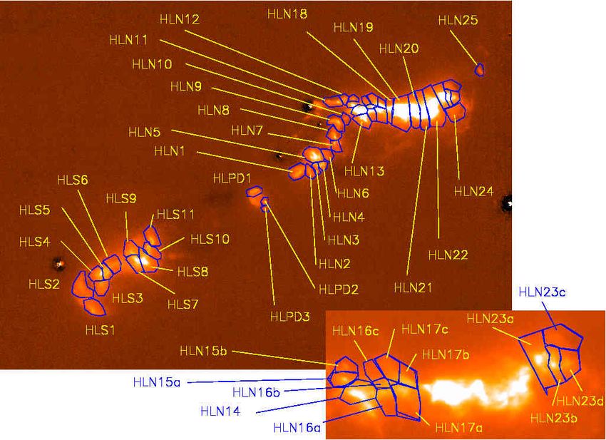
A&A proofs: manuscript no. iras20126_axv

     In high-mass star formation, the picture is observationally        onto the protostar has also been reported (Cesaroni et al. 1997;
more problematic as high-mass protostars are rare and usually           Keto & Zhang 2010; Johnston et al. 2011). The jet traced by the
far away (at kilo-parsec distances), and embedded in crowded re-        water masers over a few 100 au from the protostar appears to
gions where low-mass protostars are also present. This highlights       be co-rotating with the disc (Trinidad et al. 2005; Cesaroni et al.
the need for high-spatial-resolution observations. In addition,         2014).
studying photometric variability of a few selected high-mass-star            Imaging at infrared wavelengths (Qiu et al. 2008) suggested
precursors and their associated outflows can be a valuable tool to      that IRAS 20126+4104 was associated with an anomalously
understand how accretion occurs in these objects, circumventing         poor stellar cluster. However, subsequent X-ray observations by
the need to resolve the driving protostars. This is of course better    Montes et al. (2015) revealed an embedded stellar population
achieved when multi-epoch high-spatial-resolution observations          that hints at the existence of a richer (and possibly very young)
are available.                                                          cluster.
     In this respect, IRAS 20126+4104 is a source of great interest.         Measurements of the magnetic field orientation both at the
This massive protostar has a luminosity of ∼ 104 L (Hofner              clump scale (Shinnaga et al. 2012) and at the disc scale (Surcis
et al. 2007; Johnston et al. 2011) and is surrounded by a disc;         et al. 2014) show that the direction of the field lines is basically
this was first detected by Cesaroni et al. (1997) and confirmed by      the same from ∼ 0.2 pc to ∼ 1000 au and roughly perpendicular
subsequent higher-resolution studies (Zhang et al. 1998; Cesaroni       to the outflow axis. This suggests that the accreting material could
et al. 1999, 2005, 2014). It appears to be powering a parsec-scale      be flowing onto the star through the disc along the magnetic field
jet-outflow undergoing precession about the disc axis (Shepherd         lines.
et al. 2000; Cesaroni et al. 2005; Caratti o Garatti et al. 2008).           With all the above in mind, we think that IRAS 20126+4104 is
This jet-outflow has been imaged on scales from a few 100 au            a suitable target for high-resolution imaging at NIR wavelengths,
(see Fig. 1; Moscadelli et al. 2005; Cesaroni et al. 2013) to 0.5 pc    in order to measure the physical properties of its protostellar
(Shepherd et al. 2000; Lebrón et al. 2006) and its 3D expansion         jet, as previously undertaken, in part, by Caratti o Garatti et al.
velocity, close to the source, has been measured through maser          (2008) and Cesaroni et al. (2013). These works detected a well-
proper motions (Moscadelli et al. 2005). Two radio sources (see         collimated and structured precessing jet, with two lobes, a south-
Fig. 1) have been detected at high-spatial resolution and are asso-     eastern one (red-shifted) and a north-western one (blue-shifted),
ciated with the protostar (Hofner et al. 1999, 2007). The brighter      composed of several knots and bow-shock structures (see top
one, N1, has been detected at 3.6, 1.3, and 0.7 cm and exhibits         panel of Fig. 1), with each lobe spanning an arc of ∼ 1000 (∼
a spectral index consistent with thermal emission. It is likely to      0.08 pc). Larger field images show further distant knots which
be located ∼ 000. 3 north-west of the protostar, whose position has     are not aligned with the lobes, but they are reminiscent of a
been inferred by OH maser emission at 1665 MHz, displaying an           wiggled configuration. Wiggling is also evident in the two lobes,
elongated structure with a north-eastern-south-western velocity         suggesting that the outflowing direction is in fact precessing with
gradient reminiscent of Keplerian rotation (Edris et al. 2005).         a period whose estimates range from ∼ 1100 yr (for the closest
The fainter one, N2, has only been detected at 3.6 cm, is located       knots; Caratti o Garatti et al. 2008) to ∼ 64000 yr (for the outer
∼ 100 north-west of N1 and its morphology is reminiscent of a           flow; Shepherd et al. 2000; Cesaroni et al. 2005). A puzzling
bow shock. Radio sources N1 and N2 are roughly aligned in               feature that stands out in the images is a small (∼ 100 ) ring-like
the direction of the jet, are associated with the water maser sys-      patch (hereby, the ring-like feature or X, see Fig. 1) that mainly
tem, and have been interpreted as a manifestation of gas that has       emits in the H2 lines. This is not the circumstellar disc, which
been shocked by the jet from the protostar (Hofner et al. 2007).        appears to be heavily obscured and invisible in the NIR, but a
Another feature found is a faint radio source, S (see Fig. 1, top       structure located a few tens of arcsecs south-east of the disc,
panel), which has only been detected at 3.6 cm, and lies ∼ 100          hence facing the red-shifted lobe of the jet (see Fig. 1).
south of N1 and is roughly elongated in a direction parallel to that         We therefore targeted IRAS 20126+4104 for observations
of the jet. This has been interpreted as a distinct radio jet and its   with the second generation adaptive optics (AO) system SOUL
contribution to the outflow should be negligible (Shepherd et al.       that is nearly commissioned at the Large Binocular Telescope
2000; Hofner et al. 2007); Sridharan et al. (2005, 2007) found a        (LBT). The complex jet structure and the presence of a suitable
point-like source in L- and M-band high-resolution images co-           guide star are optimal features to test the performances of an AO
inciding with S, proving that the latter has a stellar counterpart.     system. In addition, we aimed to complement the new observa-
A clear X-ray detection was obtained with Chandra and the X-            tions with other high-resolution images available from 2000 on
ray spectrum is consistent with an embedded early B-type star           to derive, for the first time, proper motions, 3D kinematics and
(Anderson et al. 2011).                                                 photometric variability along the NIR jet of a massive protostar.
     The distance to IRAS 20126+4104 (1.64±0.05 kpc) has been                The paper layout is the following. Section 2 describes the
accurately determined from parallax measurements of water               observations and the data reduction, including all the ancillary
masers (Moscadelli et al. 2011), which prove that this is one           data. The results of our data analysis are dealt with in Sect. 3. The
of the closest discs around a B-type protostar and this allows          implications of our results are discussed in Sect. 4.
one to observe its environment with excellent linear resolution.
More recently, Nagayama et al. (2015) repeated the parallax mea-
surement with VERA, obtaining a distance of 1.33+0.19 −0.092 kpc. As
                                                                        2. Observations and data reduction
the difference with the value of Moscadelli et al. (2011) is not        2.1. SOUL AO at the LBT
statistically significant, in the following, we continue to use a
distance of 1.64±0.05 kpc.                                              SOUL (Pinna et al. 2016, Pinna et al. 2021) is the upgrade of the
     Sub-arcsecond imaging (Cesaroni et al. 2014) and model             FLAO systems (Quirós-Pacheco et al. 2010) at the LBT with an
fitting (Chen et al. 2016) have proven that the disc is undergoing      electro-multiplied camera for the wavefront sensor. As FLAO,
Keplerian rotation around a ∼ 12M protostar, as suggested by            SOUL is a single conjugated AO system, using the adaptive
the butterfly-shaped position–velocity plot obtained in almost          secondary mirror as a corrector and one natural guide star for a
every hot molecular core tracer observed. Evidence of accretion         pyramid wavefront sensor. The upgrade allows us to fully exploit
Article number, page 2 of 26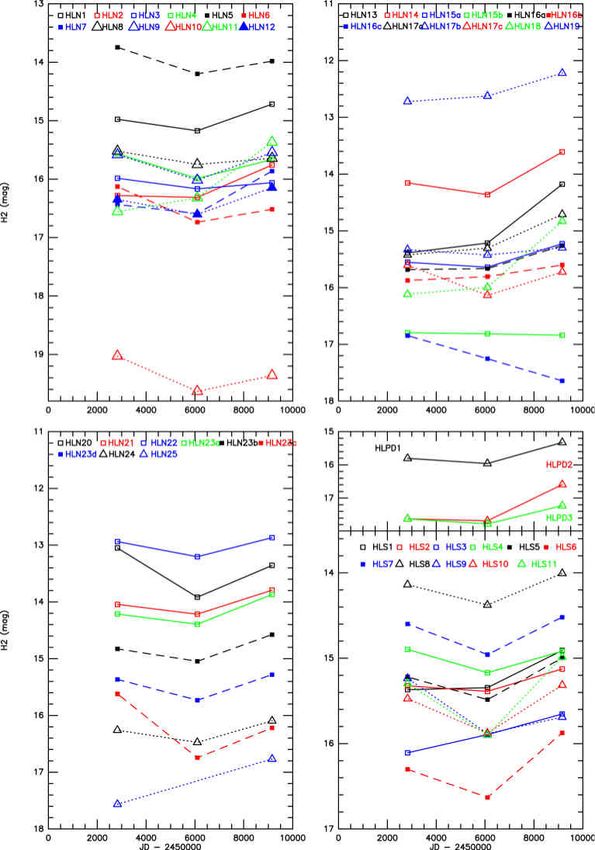
F. Massi et al.: The SOUL view of IRAS 20126+4104.

the light flux from the reference star, improving the correction.       DIT×NDIT exposures (total integration time 300 s, final PSF
In this observation, we used the R = 13.49 star (according to           width < 0.1100 ; for an accurate assessment of the PSF widths see
UCAC5; Zacharias et al. 2017) as the AO reference, which is             Appendix A) for November 2, of five DIT×NDIT exposures (total
located at the western edge of the field (Fig. 1, bottom), correcting   integration time 300 s, final PSF width ∼                      00
                                                                                                                               < 0.08 ) for November 4,
91 modes at 850 Hz.                                                     of three DIT×NDIT exposures (total integration time 180 s, final
                                                                        PSF width ∼              00
                                                                                        > 0.12 ) for November 6 (used only for calibration
                                                                        purposes). A three-colour image (red H2 filter, green K s , blue
2.2. LBT/SOUL NIR observations                                          Brγ filter) of IRAS 20126+4104 is shown in Fig. 1.
The new AO-assisted observations were carried out with the NIR               To perform photometry of the jet features, we first calibrated
imager LUCI1 at the beginning of November 2020, during the the stars in the small field of view (FoV). This was done using
commissioning time of SOUL. On-source and off-source dithered the K s images and the daophot package in IRAF. For each night
images were obtained through the narrow-band filters H2 and with K s observations, we measured the brightness of the standard
Brγ (centred at 2.124 µm and 2.170 µm, respectively), and the star FS149 in each position of the frame with different aperture
broad-band filter K s (centred at 2.163 µm) with the N30 camera radii. As the instrumental magnitude, we adopted the value at
(plate scale 000. 015 pix−1 , field of view 3000 × 3000 ). LUCI1 is which the measured brightness              00
                                                                                                                     does not change significantly any
equipped with a HAWAII-2RG HgCdTe detector with 2048 ×                  more    (aperture     radius   ∼   1.5    ).  The zero point was obtained by
2048 pixels. The K s images were obtained using the standard            averaging     the   instrumental      magnitudes       obtained at each position
double-correlated sample readout scheme (indicated as LIR in in the frame (and the standard deviation was taken as the error on
the instrument handbook), whereas the H2 and Brγ images used a the zero point), assuming - as K s standard magnitude - the value
readout scheme called MER, consisting of a set of five readings at given in the 2Mass PSC (K s = 10.052 ± 0.017).
the beginning and at the end of each integration. In addition, each          In addition, we must take into account the fact that in the
set of NDIT1 exposures through the H2 and Brγ filters was saved target images the Strehl ratio decreases with the distance to the
as a 3D FITS file with NDIT planes. A log of the observations is AO guide star (the bright star west of the target in Fig. 1, i.e. star
given in Table 1.                                                       8 in Fig. C.1). To minimise this, we analysed the radial profile of
     The target field was imaged through a sequence of dithered the stellar PSF in the frames. This is composed of a narrow peak
exposures lasting DITxNDIT each, alternating an on-source in- on top of a broader fainter feature, as expected                           (see Fig. A.1). The
tegration and an off-source one. The centre of field of each on-        broader    feature    exhibits  a  width     of ∼  0 .
                                                                                                                            00 3 (November       2 and 4) and
source frame was randomly shifted with offsets of < 3 in the   00       ∼  0 .
                                                                            00 45   (November       6), which       was   taken    as the   aperture   radius.
x and y directions of the detector reference frame. A dark area         We   constructed       the  growth     curve    for  the  bright    star lying   to the
∼ 10 away was selected as an off-source position and a dithering north of the target (star 4 in Fig. C.1), which is isolated enough,
scheme with random offsets < 10 was adopted. A standard star and we derived a correction term for the aperture photometry.
(FS149, Hawarden et al. 2001) was imaged in K s with an open Using the zero point estimated from the standard star, we derived
loop (i.e. with the AO offline) when observations were carried out the K s magnitudes of the stars in the target image. As the airmass
in this band (see Table 1) using a five-position dithering scheme difference between the target field and standard was always < 0.1,
with the star alternatively in the frame centre and in each of the no correction for airmass was needed.
four quadrants (x and y offsets of 500 ). On November 6, only
two shifted images of FS149 were taken due to poor weather 2.3. Ancillary data
conditions.
     Data reduction was performed using standard IRAF routines. In order to derive the jet proper motion and its photometric vari-
First, the frames were flat-field corrected using dome flat images. ability, we retrieved all previous H2, Brγ and K images, both
All images in each off-source 3D FITS file were averaged to- with low- and high-spatial resolution, from a number of archives.
gether in a single frame. Then, for each on-source 3D FITS file, A K image, presented in Sridharan et al. (2005), was obtained
a sky image was obtained as the median of the four nearest (in with UFTI at UKIRT from observations carried out from Au-
time) NDIT-averaged off-source images. For each on-source 3D gust 15–18, 2000 (seeing ∼ 0 . 3). Narrow-band H2, Brγ, and
                                                                                                                     00

FITS file, the single exposures were extracted, sky-subtracted, Kcont images, presented in Cesaroni et al. (2005), were obtained
corrected for bad pixels, and checked for any change in point with NICS at the TNG in June 2001 (seeing ∼ 1 . 2). Caratti o0
                                                                                                                                              00

spread function (PSF) width and in flux. Deviant frames were            Garatti   et  al.  (2008)    studied    a  further    series   of  H2,   Brγ, and K
discarded and the remaining ones were registered and averaged           images;     namely,    a dataset   (first  presented     in Sridharan     et al. 2007)
together. This was to compensate for any internal flexure from          acquired     at  the  SUBARU         telescope     with   the  Coronagraphic        Im-
the LUCI instrument during the observations. The final averaged, ager with Adaptive Optics (CIAO; Murakawa et al. 2003), used
sky-subtracted on-source images obtained from each 3D FITS as a high-resolution NIR imager, on July 10, 2003 (pixel scale
file were registered and summed together. The same scheme was of ∼ 0 . 022; seeing ∼ 0 . 9; PSF width ∼ 0 . 15), and a second
                                                                                 00                       00                          00

used for the K s frames, except that in this case the NDIT expo- dataset obtained     00
                                                                                                with NICS at the TNG on August 6, 2006 (see-
sures were not saved as 3D FITS files. In the end, the final H2 ing ∼ 1.2 ). Finally, high-spatial-resolution H2, Brγ, and K s
image was the sum of 65 exposure (total integration time DIT × images, analysed by Cesaroni et al. (2013), were obtained with
65 = 1950 s) with a PSF width ∼    < 0.1 (mostly less than 0.083 ; PISCES and the00 AO system FLAO at the LBT on June 21, 2012
                                         00                          00

measured with IRAF, for an accurate determination of the PSF (PSF width ∼ 0 . 09).
widths see Appendix A), and the final Brγ image is the sum of                Data reduction is described in the cited papers; in a few cases
40 exposures (total integration time DIT × 40 = 1200 s) with we redid it to improve the data quality and test photometric sta-
a PSF width ∼  < 0.09 . The final K s images are the sum of five bility. Notably, the CIAO, PISCES and SOUL maps roughly
                       00
                                                                        cover the same jet region around the source extending ∼ 3000 (see
 1
   A NIR image usually consists of a sequence of n single integrations Fig. 1).
of time t which are combined on-chip, where t is indicated as DIT and n      Photometry on the large FoV images (UFTI, TNG) was per-
as NDIT.                                                                formed with daophot using aperture radii ∼ 1 full width at half
                                                                                                                               Article number, page 3 of 26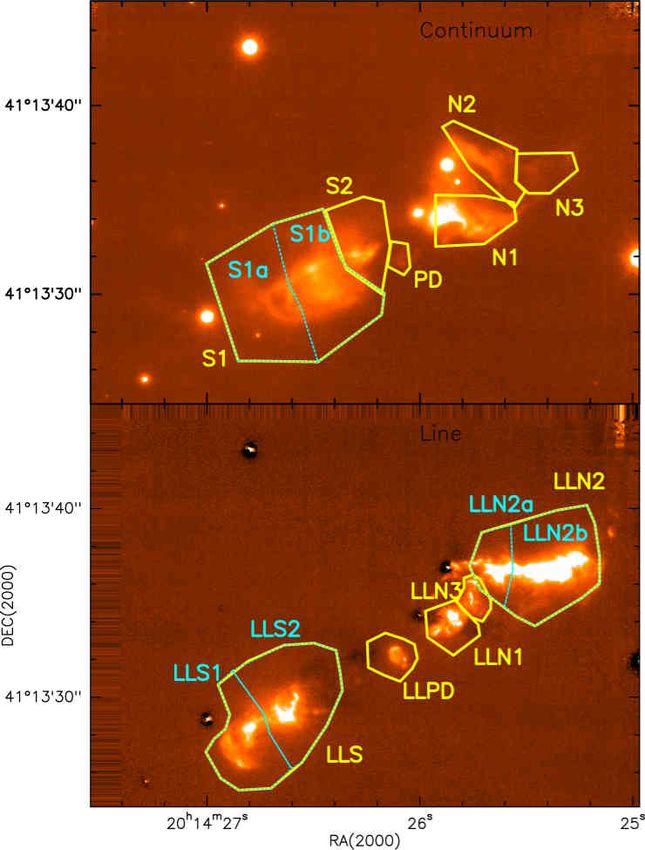
A&A proofs: manuscript no. iras20126_axv

Table 1. Observations log.

                    Filter     Target                  Date                 DIT    NDITa      Number          Number
                                                       of observations                        of on-source    of off-source
                                                       (UT)                 (s)               frames          frames
                    Ks         IRAS 20126+4104         November 2           5      12         5               5
                    Ks         FS149b                  November 2           30     1          5               0
                    Ks         IRAS 20126+4104         November 4           5      12         5               5
                    Ks         FS149b                  November 4           30     1          5               0
                    Ks         IRAS 20126+4104         November 6           5      12         3               5
                    Ks         FS149b                  November 6           30     1          2               0
                    H2         IRAS 20126+4104         November 3           30     10         7               7
                    Brγ        IRAS 20126+4104         November 4           30     8          5               5

Notes. (a) H2 and Brγ were obtained using the detector reading mode MER and all single DITs in a set of NDIT exposures are saved as a 3D FITS
file, so that each frame consists of a data-cube of NDIT planes (b) taken with an open loop

                                                                            dard stars, in these cases we only performed relative photometry
                                                                            on the stars contained in the small FoV, with aperture radii of
                                                                            the order of 1 FWHM of the broad component of the PSF to
                                                                            minimise the effects of a varying Strehl ratio.

                                                                            2.4. Continuum subtraction

                                                                            To obtain H2 and Brγ pure line emission images, we first used
                                                                            the broad-band K s and K 0 , and the narrow-band Kcont images,
                                                                            depending on the dataset. These were first rotated and shifted to
                                                                            the corresponding H2 and Brγ images using the IRAF routines
                                                                            geomap and geotran. Then we performed aperture photometry
                                                                            on the common stars (> 600 for the large FoV images, 4 − 15 for
                                                                            the small FoV AO images) in the frames to scale the images by
                                                                            assuming that the intrinsic stellar fluxes do not vary with wave-
                                                                            length, a zeroth-order approximation. We note that this implies
                                                                            that images through different filters do not need to be taken during
                                                                            the same night, as telluric extinction differences are automatically
                                                                            taken into account. Short time stellar variability might affect the
                                                                            subtraction only for the small FoV images, where the number of
                                                                            stars is low. However, the r.m.s. of the average flux ratio is ∼
                                                                                                                                           < 10
                                                                            % in these cases, which indicates no large stellar photometric vari-
                                                                            ations between pairs of images. Finally, the scaled images were
                                                                            subtracted to yield continuum-corrected images. We also note
                                                                            that when the continuum contribution is estimated from K, both
                                                                            images have to be scaled before subtraction to take into account
                                                                            that both include line emission as well as continuum emission.
Fig. 1. Three colour image (red H2 filter, green KS , blue Brγ filter) of
IRAS 20126+4104 obtained with PISCES and FLAO at the LBT in 2012          We did not notice any significant Brγ emission, so in the
(top) and LUCI1 and the new AO system SOUL at the LBT in November     end we used the available Brγ images to estimate the continuum
2020 (bottom). The KS image used for the bottom image is that taken   contribution in the H2 filter. In fact, the broad-band K filters
on November 4, that is the one exhibiting the best spatial resolution.encompass other H2 emission lines and they are therefore bound
Approximate positions of radio sources N1 (blue square), N2 (yellow   to overestimate the continuum contribution. In principle, this
square), and S (orange square, see text) are marked in the top panel with
                                                                      overestimate should be ∼ 10 %; in fact we found larger line
small coloured squares.                                               fluxes when the continuum contribution was subtracted using
                                                                      a narrow-band filter rather than the K band. However, we also
                                                                      found that the ratio of line flux (measurement with the continuum
maximum (FWHM) of the PSF. Calibration was obtained match- estimated using a narrow-band filter over the measurement with
ing the imaged stars and the 2Mass PSC and performing a linear the continuum estimated using the K band) increases when the
fit. The fit formal error is typically < 0.2 mag (∼ 0.08 for UFTI), ratio of the line to continuum (K) flux in a knot decreases. This
but one has to consider that this includes intrinsic variability in a indicates that the line flux may be significantly underestimated
number of stars and the zero point is then expected to be more for faint line emission superimposed on a strong continuum (K)
accurate than ∼ 0.1 mag. As neither the CIAO images nor those flux when the continuum contribution is evaluated using the K
obtained with PISCES are associated with observations of stan- band (see Appendix G).
Article number, page 4 of 26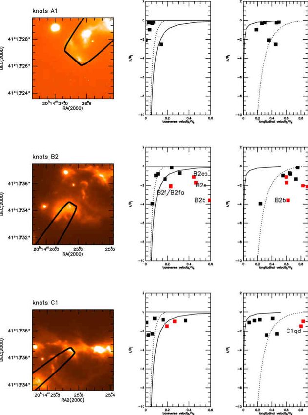
F. Massi et al.: The SOUL view of IRAS 20126+4104.

2.5. Jet photometry
We performed photometry of the jet emission, both in the con-
tinuum and in the H2 2.12 µm line, using the task polyphot in
IRAF. We divided the jet into smaller components and defined
a polygon for each one, taking care of encompassing most of its
emission (down to a ∼ 5σ level of the background as determined
far from the jet). Before doing the photometry, we registered and
projected all of the images onto the SOUL H2 frame grid as ex-
plained in Appendix B, so we did not have to adapt the polygons
to each image. The photometric zero points have been computed
for each frame based on two bright stars which are common to
all images. The variability of the two stars, the stability of the
zero points, and the consistency of the calibration are discussed
in Appendix C, D, E.
     As for continuum emission, the selected polygons are de-
scribed in Appendix F and shown in Fig. 2. Where possible, it
was measured on the Brγ-filter images, which do not include the
H2 line emission and where Brγ emission has not been detected.
Only in two cases did we use K images (UKIRT 2000 and TNG
2006) after subtracting the derived H2 line emission (we used
TNG 2001 to estimate the correction for UKIRT 2000). For the
lower-resolution images (UKIRT and TNG), we also subtracted
the stars in the frames by using daophot before performing the
photometry. The sources of error involved in the various steps of
the photometry are assessed in Appendix F.
     Photometry of the jet emission in the H2 2.12 µm line was
performed in the same way as was done for continuum emission.
However, in this case we used two different sets of polygons.
First, we defined a set of larger polygons (see Appendix G and
Fig. 2.) to exploit both the higher and the lower spatial reso-
lution images. Where possible we used the pure line emission           Fig. 2. Jet decomposition in polygons. Top panel. Brγ-filter image of
images obtained by subtracting the continuum contribution as           IRAS 20126+4104 obtained with LUCI1 and the AO system SOUL,
estimated from adjacent narrow-band filters. In only one case          overlaid with the polygons used for the photometry in the continuum.
was the correction estimated from the broad-band K 0 filter. As        The adopted designation is labelled. We note that polygon S is composed
shown in Appendix G, while narrow-band filters (namely Brγ             of S1 and S2, and S1 is further subdivided into S1a and S1b. Bottom
and Kcont ) yield a consistent continuum correction, using broad-      panel. Pure H2 line emission image of IRAS 20126+4104 obtained with
band K images results in more discrepant continuum corrections         LUCI1 and the AO system SOUL, overlaid with the polygons used for
compared to Brγ, leading to increasingly fainter magnitudes in         the jet photometry. The adopted designation is labelled. We note that
                                                                       polygon LLS is composed of LLS1 and LLS2, and LLN2 is subdivided
the line emission with increasing continuum contamination.
                                                                       into LLN2a and LLN2b.
     Next, we analysed the high-spatial-resolution pure H2 line
emission images from the AO-assisted observations to identify
single emission knots and defined a set of smaller polygons en-     that the proper motions are essentially derived in the reference
compassing each knot (see Fig. 3 for designation). In this case, we frame of the protostar (see Appendix B). To compute the proper
only used the high spatial resolution images (CIAO 2003, PISCES     motions (PMs), we used the same strategy and our own developed
2012, and SOUL 2020) with the continuum correction derived          software in python as described in Caratti o Garatti et al. (2009).
from the Brγ images. To focus only on the smaller-scale struc-          Briefly, single shifts were computed between image pairs
tures, we adapted the multi-scale image decomposition described     (namely the SOUL image versus previous PISCES and CIAO
in Belloche et al. (2011), with seven levels of decomposition,      images) keeping the latest epoch as a reference and using a cross-
to filter out large-scale emission structures. This should have re- correlation method. After identifying each knot or structure in
sulted in the efficient filtering out of ∼  00
                                         > 2 structures and a bettereach image, a sub-image, enclosing the structure 5 σ contour, was
background estimate. We note that the shape and location of a       selected and cross-correlated with the corresponding sub-images
few polygons of this second set had to be slightly changed and      obtained from the earlier epochs. In a given pair of sub-images,
adapted depending on the image because of the knots’ proper         the earlier one was then shifted in steps of 0.1 pixel in x (R.A.) and
motions.                                                            y (Dec.), and for each shift (∆x, ∆y) a product image was created.
                                                                    The highest-likelihood shift for each epoch is that yielding the
2.6. Proper motion analysis                                         maximum correlation signal f (x, y) integrated over the considered
                                                                    structure on the corresponding product image. To quantify the
We used the H2 continuum-subtracted high-angular resolution im- systematic errors for the shift measurements, the size and shape
ages from CIAO, PISCES and SOUL after flux calibration based of each sub-image that encloses the considered structure was
on the photometric zero points (see Sect. 2.5), and registration to varied. The resulting range of shifts gives the systematic error,
and projection onto the SOUL H2 frame grid (Appendix B) to which depends on the structure signal-to-noise ratio (S/N), shape,
infer proper motions of knots and bow shocks along the jet. This and time variability. This uncertainty is typically much larger
dataset provides a time baseline of more than 17 years. We note than the register error. Finally, the PM value of each structure was
                                                                                                                 Article number, page 5 of 26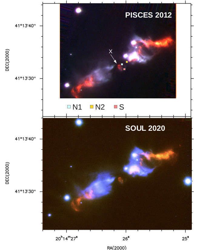
A&A proofs: manuscript no. iras20126_axv
Fig. 3. Pure H2 line emission image of IRAS 20126+4104 obtained with LUCI1 and the AO system SOUL, overlaid with the polygons used for the
high-spatial-resolution jet photometry.
derived from a weighted least square fit of the shifts derived for 3.2. Continuum variability
each epoch, fitting the motion in R.A. and Dec. simultaneously.
This fit also provides the associated errors. The results of the fits We found the most remarkable flux variations in the continuum
are detailed in Appendix I. emission. To analyse such variability, we selected seven con-
tinuum emitting regions: three in the north-western and south-
eastern cavity, respectively, and one enclosing the ring-like feature
3. Results close to the source position (see Appendix F and Fig. 2). The light
curves of these regions are displayed in Fig. 4. The figure shows
3.1. Morphology of the jet and outflow cavities a clear decrease of the continuum emission in the north-western
The three-colour image (red H2 filter, green KS , blue Brγ filter) lobe between 2000 and 2006 (see also Fig. 5, upper and bottom
obtained from the SOUL data, shown in the bottom panel of left panels, and the short movie in Fig. H.1 in Appendix H), with
Fig. 1, is quite similar to the PISCES one presented in Fig. 1 of a subsequent increase. Conversely, the south-eastern lobe seems
Cesaroni et al. (2013), which has been adapted in the top panel to have brightened up during the same time interval and then to
of Fig. 1. The continuum emission (Brγ and K s filters) delineates have decreased in intensity. The ring-like feature (labelled PD in
the outflow cavities (in blue and cyan), which scatter the radiation Fig. 4) appears to exhibit a slow steady flux decrease.
from the central source, which is undetected at 2 µm. The H2
shocked emission traces a precessing jet (in red; see also Caratti 3.3. H line variability
2
o Garatti et al. 2008), which is highly fragmented, especially
towards the north-western blue-shifted side, displaying a large The line photometry on the set of larger polygons (including
number of knots and bow shocks. It is worth pointing out that the low spatial resolution images; see Appendix F and Fig. 2) is
our high-resolution images show only the inner portion of the shown in Fig. 6. We note that, as discussed in Appendix G, the
flow (∼30 00 in size or ∼0.24 pc), which extends further north and fluxes of the data points obtained by correcting the continuum
south (see, e. g. Shepherd et al. 2000, Lebrón et al. 2006). contamination using the K 0 image are expected to be underesti-
To study the jet variability and kinematics, each sub-structure mated, so the dip displayed in the plot on JD 2453953 (black solid
(knots and bow shocks) showing local emission peaks above squares) is likely not real. A very rough correction of 0.3 mag
5 σ was identified and labelled in the SOUL H2 continuum- (open triangles in the figure), which should represent an upper
subtracted image. In our kinematical analysis we followed the limit, has been obtained following Appendix G. Furthermore,
general nomenclature used by Caratti o Garatti et al. (2008), who the obtained magnitudes need to be corrected for the different
divided the flow regions into six different groups: A1, A2, X, B, bandwidths of the H2 filters (see Appendix G). We adopted the
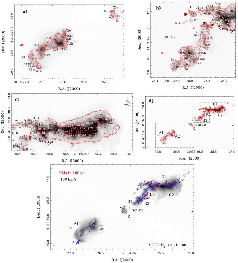
C1, and C2 (see also Fig. 8d). LUCI1 filter bandwidth as a standard and corrected all other mea-
Article number, page 6 of 26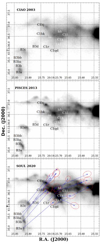
F. Massi et al.: The SOUL view of IRAS 20126+4104.

                                                                        hand, two knots exhibit a decrease of at last ∼ 0.5 mag, that is
                                                                        HLN16c and HLN23c, and they are located in outer areas of C1.
                                                                             An increase in line emission implies an increase in the column
                                                                        density of molecules in the upper level of the transition integrated
                                                                        over the knot area. In bow shocks, this column density increases
                                                                        with increasing shock speed in the range ∼ 5 − 15 km s−1 (Tram
                                                                        et al. 2018). A generalised trend of brightening therefore sug-
                                                                        gests that more and more gas is being entrained into the shocked
                                                                        regions.
                                                                             Due to the shape of the PSF in the AO-assisted images, the
                                                                        filtering is bound to cause some of the smaller-scale flux to be
                                                                        missed since a residual small fraction of the PSF flux is spread
                                                                        on a larger size compared to the PSF diffraction-limited peak.
                                                                        Thus, it is essential to ensure that this does not affect the time
                                                                        variations displayed by the single knots as well. By redoing the
                                                                        same photometry on the unfiltered images, we found the same
                                                                        trends as from the filtered images, with the main difference being
                                                                        that the knots are a few tenths of magnitude fainter in the filtered
                                                                        images (down to ∼ 1 mag fainter in only a few cases). So we can
                                                                        confirm that the flux from most knots is stable within a few tenths
                                                                        of magnitude, with some exceptions.

                                                                        3.4. Proper motion, kinematics and dynamical age of the H2
                                                                             jet

                                                                          Figure 8 (a-d panels) displays the knots identification and their
                                                                          measured proper motions (PMs; panel e) as derived from the
                                                                          analysed H2 continuum-subtracted images at high-spatial resolu-
                                                                          tion (see Sect. 2.6). The shifts of some of the knots are evident
Fig. 4. Photometric variability of the continuum features defined in in the short movie of Fig. H.2 in Appendix H. Thanks to the
Fig. 2. We note that N and S indicate the northern and southern lobe, extremely high-spatial resolution of our images and their 17-year
respectively, and PD is the ring-like feature. The numbers increase from time baseline, we were able to measure knot PMs down to a few
south-east to north-west. We note that S is further subdivided into S1
and S2, and S1 is in turn subdivided into S1a and S1b. The symbol size
                                                                          milliarcseconds (mas) per year. These values range from ∼2 to
                                                                                       −1
is ∼ 0.2 mag in the vertical direction, which is comparable with the ∼20 mas yr . The results are listed in Table I.1 of Appendix I. In
photometric errors. A sinusoid of period ∼ 12 yr is overlaid on the N1    particular,  the table provides knot IDs, coordinates (as derived
                                                                                                                             −1
light curve. The same, but with a phase shift of π, is also drawn in the from the SOUL map), proper motions (in mas yr ), tangential ve-
bottom box.                                                               locities (at a distance of 1.64 kpc) and position angles (PAs, from
                                                                          north to east) of the corresponding vectors, and their uncertainties.
                                                                          The blue arrows in Fig. 8 (panel e) show the average displacement
surements using Eq. (D.10) and Eq. (D.11). The line flux can of each knot in 100 years along with its uncertainty (red ellipses).
be derived from the magnitude m given in the figure through the Overall, both blue-shifted (B and C groups) and red-shifted (X
following:                                                                and A groups) structures along the jet move away from the source
                                                                          position, roughly following the precession pattern described in
F = 1.06 × 10−15 × 10−0.4m W cm−2 .                                   (1) Caratti o Garatti et al. (2008) (see also their Figure 11).

As we cannot rule out systematic errors in the zero points of                 On average, velocities increase moving farther away from the
∼ 0.1 − 0.2 mag in an unknown direction, the maximum variation source position (groups B1, B2 and B3 on−1the blue-shifted side
intervals of ∼< 0.4 mag per polygon indicate that the total energy with average 3tg ∼ 69, 107, and 115 km s and groups X and               −1
emitted in the 2.12 µm line is probably almost constant in time A2 on the red-shifted side with average 3tg ∼ 40 and 70 km s )
within a few tenths of magnitude in the sampled regions.                  until they  drop   as the flow encounters  a slower   group moving
                                                                                                                                            −1
    The knot line variability on the smaller scale (excluding the ahead (i. e. group C1 and A1 with average 3tg ∼ 64 and 55 km s ,
lower spatial resolution images; see Fig. 3 for polygon designa- respectively) and collide against it (see Fig. 9). Our analysis of
tions) is shown in Fig. 7. Most knots exhibit a constant flux within the 3D velocities (see Sect. 4.1) confirms that this is not just a
∼ 0.2 − 0.4 mag from 2003 to 2020 in a similar trend as found projection effect.
from the low spatial resolution photometry. Nevertheless, even                The clearest example is shown in Fig. 10. The fast flow in
assuming zero point systematic errors of ∼ 0.2 mag in opposite the B3 region is moving at 3tg ∼100–120 km s−1 (see e. g. knots
directions, variations > 0.4 mag should be considered as real. In B3c and B3bb) and shocks against the C1hi, C1hj, and C1hk
this respect, an emission increment ≥0.8 mag is evident for knot regions (3tg ∼10−70 km s−1 , corresponding to polygons HLN13
HLPD2 in the ring-like feature, the outermost north-western knot and HLN14 in Fig. 3), producing a bow shock (knots C1hi, hk,
(HLN25), knot HLN11 adjacent to star 6, knot HLN13 connected hh, k, and k1), which increases in brightness from the 2003 to
with bow-shock C1h and C1k (see Sect. 4.2), and knot HLN18 in the 2020 epoch (middle and bottom panels of Fig. 10, see also
the middle section of C1 (see Fig. 8). Another five knots exhibit the short movie of Fig. H.2 in Appendix H). Indeed, one can see
an increase of ∼ 0.5 mag, namely HLN2, HLN14, and HLN19 from Fig. 7 that these two H2 emitting regions are among those
and, in the south, HLS1 and HLS3 (see Figure 7). On the other displaying the largest increase in luminosity (about 1.6 mag).
                                                                                                                  Article number, page 7 of 26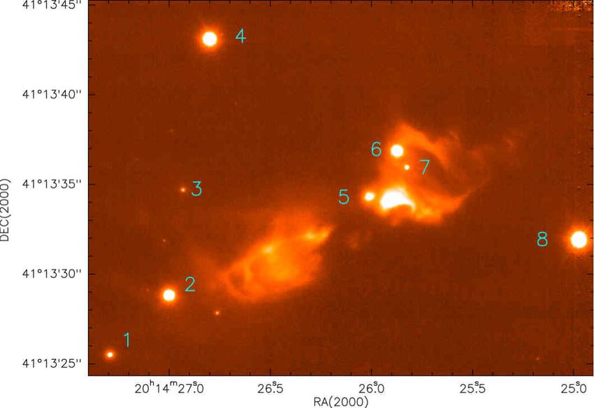
A&A proofs: manuscript no. iras20126_axv

Fig. 5. Comparison of the continuum emission throughout the various observed epochs. This has been approximated with the Brγ-filter images,
except for the runs of July 2000 and August 2006 where broad-band K images corrected for line emission have been used. The flux levels have been
adjusted so that the mean of the counts of stars 2 and 4 is the same in all frames. The dimming of the northern lobe (especially region N1) and the
simultaneous brightening of the southern lobe in July 2003 are evident.

    The average tangential velocity of the H2 flow is                     Group X (the ring-shaped region close to the source, labelled as
80±30 km s−1 . Here the reported uncertainty is the standard de-          PD in our photometry analysis) has a similar dynamical age as
viation over the whole sample. In fact, by analysing the velocity         B1 (τ̄X =280±50 yr), whereas the τ̄ value of the farthest group
vectors of all sub-structures in a group, it is clear that tangential     towards the north-west (C2) is roughly consistent with that of
velocities and position angles exhibit large spreads (namely tens         A1, namely τ̄C2 =1070±300 yr. This might indicate that the A1
of km s−1 and degrees, i. e. much larger than the velocity uncer-         group decelerated, as is also hinted at by the presence of a large
tainty of each single knot) within the same group (see bottom and         bow shock at the front of the group. The large uncertainty on τ̄ of
middle panels of Fig. 11). In addition, the scatter in velocity is        some groups reflects the large scatter in tangential velocities of
larger in those regions where knots are more crowded and shocks           the groups as seen in Fig. 11, in particular for groups A1, A2, B3,
are therefore expected to interact with each other. This reflects         C1, and C2, namely where the dynamical interaction between
and possibly causes the observed fragmentation along the flow.            knots may be more important.
    There are other interesting features arising from the proper              One puzzling feature displayed by the PM vectors is that the
motion analysis of the different regions along the jet. Group X,          average direction of the farthest knots (A1, C1, and C2) does not
corresponding to the ring-like feature (PD) and as the H2 region          intersect the current location of the protostar, but passes north-
closest to the source position, looks like a structured expanding         east of it. If a line coinciding with the proper motion direction of
ring with the exception of knot X2 (polygon HLPD2 in Fig. 3),             the protostar is drawn, the average directions of the knot proper
which first appeared in the 2012 image and increased in lumi-             motions cross it at the earliest locations (C1 and C2 ∼ 100 − 200
nosity by 2020. The expansion is clearly visible from the vectors         north-east of the protostar and A1 and A2 ∼ 300 north-east of
in Fig. 8 and from the large scatter in their position angles (see        the protostar), in accordance with them being ejected at earlier
middle panel of Fig. 11). On the other hand, knot X2, which first         epochs (see Fig. 13). However, the knot PMs have been derived in
appeared in the 2012 image as well, is not co-moving with the             a reference frame that appears to be similar to that of the protostar
expanding ring-like feature but it is rather moving straight away         (see Appendix B), so such an effect should not be detected in our
from the source position.                                                 analysis. One possible explanation is that the protostar proper
    By combining proper motions and projected distance (d) to             motion has decreased (in absolute value) with time.
the source, we also estimated the dynamical age (τ=d/PM; in
yr) of each knot. Values are reported in Column 8 of Table I.1
and plotted against their projected distance to IRAS 20126+4104           4. Discussion
in the top panel of Fig. 11. The dynamical ages provide a raw             4.1. H2 3D kinematics
estimate for the ejection time. Actually they provide a lower limit,
if matter actually accelerates soon after its ejection, as Fig. 9         By combining the tangential velocities (3tg ) derived in this work
would suggest. Figure 12 shows the average dynamical age of               with the H2 radial velocities (3r ) obtained at high-spectral reso-
each group of knots versus their average projected distance to the        lution (R=18 500) with UKIRT/CGS4 by Caratti o Garatti et al.
protostar. Notably, all the knots have been ejected recently. Their       (2008), we are able to infer both the total velocity (3tot ) and the
average τ (τ̄) ranges from 220±50 yr for group B1 along the jet           inclination of its vector with respect to the line of sight (i) for
to 2200±900 yr for the farthest group A1 towards the south-east.          the knots encompassed by the CGS4 slit. It is worth noting, how-
Article number, page 8 of 26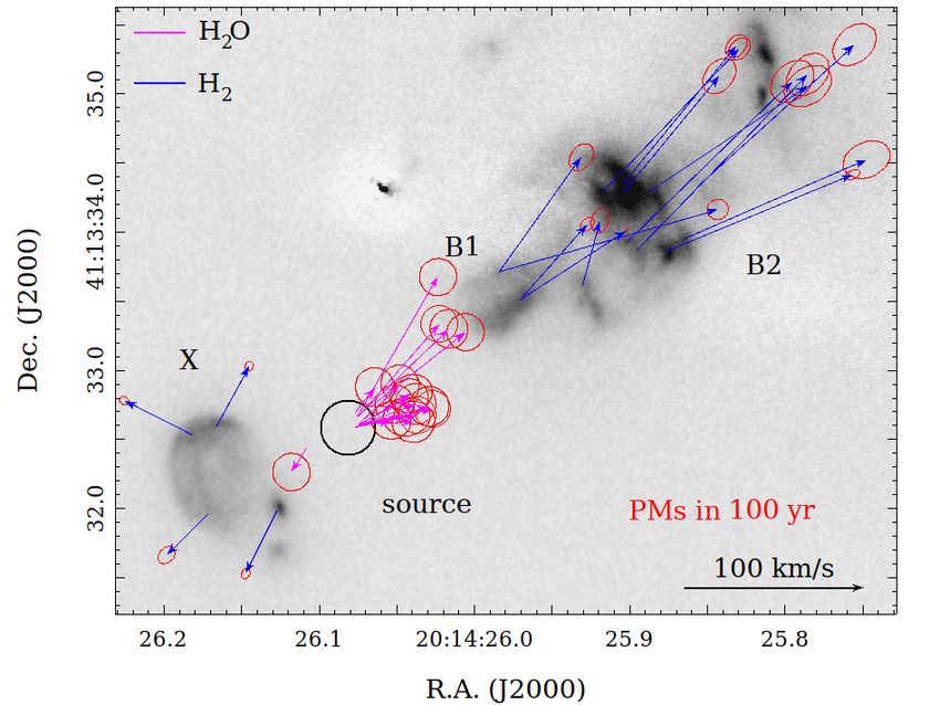
F. Massi et al.: The SOUL view of IRAS 20126+4104.

                                                                                The results are shown in Table I.2 of Appendix I, where the
                                                                                identified substructures with total velocities and inclination i with
                                                                                respect to the line of sight are listed. The inclination i of vectors
                                                                                in both lobes ranges from 76◦ to 98◦ with respect to the observer,
                                                                                yielding a weighted-mean inclination with respect to the plane
                                                                                of the sky of i sky =8◦ ±1◦ . This result is consistent with the value
                                                                                i ∼ 80◦ derived from the H2 O maser measurements obtained
                                                                                (towards the blue-shifted lobe) close to the source by Moscadelli
                                                                                et al. (2011). Our results therefore confirm that the outflow axis
                                                                                lies close to the plane of the sky at spatial scales ranging from
                                                                                a few hundred mas to ∼ 1000 . The ∼10◦ spread in the i values of
                                                                                the knots might arise from the jet precession or it might indicate
                                                                                that our original assumption in associating each peak 3r to the
                                                                                3tg of the corresponding brightest substructure is not completely
                                                                                correct. In any case, such a spread does not really affect the fact
                                                                                that the reported tangential velocities of the knots can be assumed
                                                                                equal to the total velocities (3tg / sin i ' 3tg ' 3tot ) within a 3%
                                                                                uncertainty in the worst-case scenario (i. e. i=76◦ towards group
                                                                                C2).

                                                                                4.2. Bow shocks
                                                                                We tested our data to check that the H2 emission (morphology,
                                                                                fluxes, and projected velocities) of at least some knots is con-
                                                                                sistent with being originated in bow shocks. We performed two
                                                                                tests based on a comparison with model predictions. In the first
                                                                                test, the morphology, size, and brightness of the H2 knots were
                                                                                compared with magneto-hydrodynamic (MHD) models of bow
                                                                                shocks. As an example, we considered knots A1, B3c, and C1h-
                                                                                C1k, as well as the 3D bow-shock models of Gustafsson et al.
Fig. 6. Photometric variability of jet areas in the H2 2.12 µm line emis-
                                                                                (2010). We converted the knot photometry into brightness by
sion. We note that LLN and LLS indicate the northern and southern
lobe, respectively, and PD is the ring-like feature (see Fig. 2).In addition,   using the 2MASS zero magnitude flux at K s , a filter width of
LLS is further subdivided into LLS1 and LLS2, and LLN2 is in turn               0.023 µm (see Table D.1), and the solid angle of the relevant
subdivided into LLN2a and LLN2b. The small open triangles (connected            polygons (correcting for extinction by adopting the AV values
with dotted lines) indicate the fluxes with continuum subtraction from          derived by Caratti o Garatti et al. 2008). The morphology of the
the K 0 band when corrected following Appendix G. The photometric               selected knots is clearly reminiscent of that of bow shocks from
errors are smaller than the symbol sizes. The magnitudes have been              a flow parallel to the plane of the sky. As for A1, both its width
corrected for bandwidth differences.                                            (∼ 4000 au) and its average brightness (∼ 1−2×10⁻⁶ W m−2 sr−1 )
                                                                                roughly agree with a modelled bow shock impacting a medium
                                                                                of density ∼ 105 cm−3 with a speed of 50 − 60 km s−1 . Since the
ever, that the spectral images of CGS4 have a spatial resolution
                                                                                actual speed that we have derived is ∼ 45 km s−1 , A1 is likely
one order of magnitude worse (slit width 000. 5, seeing ∼ 100 ) than
                                                                                to represent a terminal shock. The width (∼ 800 au) and average
the high-resolution images used here. As a result, the spectra
                                                                                brightness (∼ 9 × 10⁻⁷ W m−2 sr−1 ) of B3c again points to a bow
extracted by Caratti o Garatti et al. (2008) typically encompass
                                                                                shock propagating in a medium of density ∼ 105 cm−3 with a
more than one substructure and more than one velocity com-
                                                                                speed of 50 − 60 km s−1 . Finally, C1h-C1k has a width of ∼ 1600
ponent is detected as well (see their Fig. 8 and Table 4). To
                                                                                au and an average brightness of ∼ 0.4 − 1 × 10⁻⁵ W m−2 sr−1 ,
associate radial and tangential velocities of each region, the spa-
                                                                                which is consistent with a bow shock propagating in a medium of
tial resolution of the CIAO image (closest in time to the spectral
                                                                                density ∼ 105 − 106 cm−3 with a speed of 50 − 60 km s−1 . We note
data) was first degraded to 100 to match that of the spectral im-
                                                                                that the models of Gustafsson et al. (2010) are able to reproduce
ages of UKIRT/CGS4. Then, slit-like areas were cut out of the
                                                                                some of the asymmetry exhibited by the knots on the basis of the
degraded image and the corresponding 1D profiles were extracted
                                                                                magnetic field direction both on the plane of the sky and along
and matched to those extracted from the CGS4 spectral images.
                                                                                the line of sight. The magnetic field strength in the models of
We then assumed that the peak intensity of the extracted spectra
                                                                                Gustafsson et al. (2010) selected here range from between 500
originated from the brightest knot-substructure encompassed by
                                                                                and 5000 µG. It is worth noting that the most remarkable discrep-
the slit and combined its radial velocity with the tangential ve-
                                                                                ancy between observations and models in the specific cases of
locity of that knot or substructure (given in Table I.1). The total
                                                                                B3c and C1h-C1k is the measured knot velocity, which exceeds
velocity and inclination of each knot are then as follows:
                                                                                the hydrogen dissociation limit (∼ 60 km s−1 ). Indeed, most of
         q                                                                      the observed knot velocities exceed such a value (see Table I.1).
3tot =       32tg + 32r                                                  (2)    The most likely explanation, as already mentioned, is that these
                                                                                features represent internal shocks, in other words that the flow
                                                                                here is impacting a parcel of gas already in motion, resulting in a
               !                                                                lower relative velocity. As a consequence, the measured tangen-
           3tg                                                                  tial velocities (and thus total velocities) can be greater than the
i = arctan       .                                                       (3)    actual shock velocities.
           3r
                                                                                                                         Article number, page 9 of 26
A&A proofs: manuscript no. iras20126_axv Fig. 7. Photometric variability of jet knots in the H2 2.12 µm line emission. We note that LHN and LHS indicate the northern and southern lobe, respectively, and LHPD is the ring-like feature (see Fig. 3). The magnitudes have been corrected to the LUCI1 H2 filter bandwidth. Article number, page 10 of 26
F. Massi et al.: The SOUL view of IRAS 20126+4104.

Fig. 8. Knot identification in the SOUL H2 continuum-subtracted image of the IRAS 20126-4104 flow and knot proper motions. Panel a): Zoom-in
on the A and X knot regions (red-shifted lobe). Contour levels at 5, 7, 10, 15, 20, and 25 σ are overlaid. We note that 1 σ corresponds to
8×10⁻²³ W cm−2 arcsec−2 . Panel b): Zoom-in on the B and C1 knot regions (blue-shifted lobe). Contour levels at 5, 7, 10, 15, 30, and 40 σ are
overlaid. Panel c): Zoom-in on the C1 and C2 knot regions (blue-shifted lobe). Contour levels at 5, 10, 20, 30, 40, 50, 60, 80, and 120 σ are overlaid.
Knot peaks are indicated by white dots. Panel d: Overall view of the IRAS 20126+4104 flow close to the source. The main structures as reported
in Caratti o Garatti et al. (2008) are labelled. Panel e: Proper motions (PMs) with their uncertainties (blue arrows and red ellipses) in 100 yr of
structures and sub-structures along the H2 jet in IRAS20126+4104. The actual observed shifts are approximately one fourth the length of the
corresponding arrow. The red circle marks the position (along with its uncertainty) of the protostellar continuum emission at 1.4 mm (Cesaroni et al.
2014). The main structures as labelled in Caratti o Garatti et al. (2008) are also indicated.

                                                                                                                       Article number, page 11 of 26
A&A proofs: manuscript no. iras20126_axv
Fig. 9. Average tangential velocity vs average projected distance to the
source for each group of knots.
In the second test, we compared knots A1, B2, and C1 with
the ballistic bow-shock model of Ostriker et al. (2001). In order
to derive the proper coordinate system used by those authors (i.e.,
distance z from the head of the shock along the jet axis and dis-
tance R from the jet axis), we have developed a software routine
that fits their Eq. (22) to the outermost shape of H2 emission struc-
tures resembling bow shocks. For the sake of simplicity, the fit
assumes the jet to lie in the plane of the sky (a good assumption,
as discussed in Sect. 4.1), a bow-shock speed 3s = 150 km s−1 ,
a sound speed Cs = 8 km s−1 (which is appropriate for a gas
temperature of 10000 K), and β = 4.1 (Sanna et al. 2012). The fit
yields the coordinates of the head of the shock (the centre of the
working surface), the projected orientation of the shock axis, and
R j , the radius of the inner driving jet (and of the working surface).
Using Table I.1, one can now compute the coordinates (R, z) of
the associated knots in the bow-shock reference frame and the
components of their projected speed parallel (longitudinal) and
perpendicular (transverse) to the jet axis. In turn, these can be
compared with the ones predicted by the model (Eqs. 18, 19, 20,
21 of Ostriker et al. 2001). In particular, given a knot associated
with a bow shock, its projected velocity component perpendicular
to the jet axis should fall between zero and the predicted radial
speed of the outer surface layer at the same distance z from the
shock head, whereas the knot-projected velocity component par-
allel to the jet axis should fall between the predicted mean shell
and outer surface layer longitudinal speeds at the same distance z
from the shock head. The comparison and the spatial distribution
of the shock envelope from the fit is displayed in Fig. 14 for knots
A1, B2, and C1. The results of the fit are also listed in Table 2.
Figure 14 shows that the morphology of knots A1, B2, and C1 is
well fit by the bow-shock outer-shell model. The proper motions
of the knots making up group A1 appear to be consistent with
the model prediction. As for C1, the velocity plots indicate that
the location of the working surface at the head of the shock has
probably not been estimated correctly and that it should be shifted
a little backwards along the jet. After this correction, the proper
motions of the knots making up C1 are consistent with the model
predictions as well (possibly except for knot C1qd). Some of the
proper motions of the knots making up B2 are consistent with the
model predictions, while others are not. In this case, one has to Fig. 10. Evolution of the bright bow shock in the C1h and C1k regions.
take into account that the region around B2 displays a complex The top, middle and bottom panels show the same area of the sky at
pattern of shocks, thus the matter along the jet axis is proba- the three different epochs (2003, 2012, and 2020). The fast moving flow
bly soon entrained in other internal shocks due to subsequently (3tg ∼100–120 km s−1 ) corresponding to B3 shocks against the C1h and
ejected matter. In this respect, knot B2b, the most diverging one, C1k regions (3tg ∼10–70 km s−1 ) producing a bright bow shock. The
is clearly a bright isolated patch of emission (see Fig. 8) located PMs of knots are shown as in Figure 8.
at the border of the fitted shock outer shell, marking a different
shock episode with high probability.
Article number, page 12 of 26F. Massi et al.: The SOUL view of IRAS 20126+4104.
C2
C1
B3
B2
B1
A2
A1
Fig. 11. Tangential velocity (bottom panel), position angle (middle
panel), and dynamical age (top panel) vs distance to the source for
each knot. Red labels show knots in the C1 group that might belong to a
different flow (see text). Fig. 13. Mean directions of the proper motion vectors in the blue-shifted
lobe (top panel) and in the red-shifted lobe (bottom panel). The proper
motion track of the protostar is marked by the red line and its current
location by the red cross. Clearly, the more distant the knot group is from
the protostar, the more distant (to the north-east) the intersection of its
mean direction is with the track. The protostar is moving towards the
south-west.
Table 2. Shape of three possible bow shocks (from fitting Eq. (22) of
Ostriker et al. 2001).
knot 3s Cs β θ Rj α
ID (km s−1 ) (km s−1 ) (◦ ) (au) (◦ )
A1 150 8 4.1 141.15 1237 4
B2 150 8 4.1 −30.4 469 5.5
C1 150 8 4.1 −49.25 349 2
Notes. Column 2: assumed bow-shock speed; column 3: assumed sound
speed; column 4: assumed β; column 5: jet axis position angle; column
Fig. 12. Average dynamical age vs average distance to the source for 6: inner jet radius; column 7; angle to the driving source subtended by
each group of knots. R j.
Interestingly, the method also provides an estimate of the scattered dust emission from the cavity dug by the protostellar
aperture angle of the jet from the radius of the inner jet driving jet is visible on both sides. This is consistent with a jet lying
the bow shock. The values obtained range from between 2 − 5.5◦ almost on the plane of the sky (as confirmed by our measured 3D
(half aperture, see Table 2), which is slightly less than the value velocities, see Table I.2), with a large enough opening angle (half
obtained from the water masers (∼ 9◦ ; Moscadelli et al. 2011). In opening ∼ 9◦ according to the water maser motion modelling
addition, the bow-shock axes derived from A1 and C1 intersect by Moscadelli et al. 2011). The relatively bright double-sided
the proper motion track of the protostar north-east of it, as found cavity, compared to the nearby fainter source S suggests that the
for the average proper motion directions. protostar may be located near to the front surface of its parental
molecular clump, which could explain the low extinction towards
both cavities.
4.3. Jet precession
The proper motion analysis confirms that all the H2 features
A comparison between the continuum emission and the H2 line in the north-western lobe are moving away from areas close to
emission in Fig. 1 clearly indicates that continuum emission the protostar location. In particular, the proper motions of group
(outlined by the blue-coloured emission) is detected on both the B knots agree well both in speed and direction with those of the
blue-shifted and the red-shifted sides of the outflow, meaning that cluster of water masers, which are closer to the protostar location
Article number, page 13 of 26You can also read