The Solar ALMA Science Archive (SALSA) - First release, SALAT, and FITS header standard - Astronomy & Astrophysics
←
→
Page content transcription
If your browser does not render page correctly, please read the page content below
A&A 659, A31 (2022)
https://doi.org/10.1051/0004-6361/202142291                                                                        Astronomy
c ESO 2022                                                                                                          &
                                                                                                                   Astrophysics

                           The Solar ALMA Science Archive (SALSA)
                             First release, SALAT, and FITS header standard?
           Vasco M. J. Henriques1,2 , Shahin Jafarzadeh1,2 , Juan Camilo Guevara Gómez1,2 , Henrik Eklund1,2 ,
               Sven Wedemeyer1,2 , Mikołaj Szydlarski1,2 , Stein Vidar H. Haugan1,2 , and Atul Mohan1,2

      1
          Rosseland Centre for Solar Physics, University of Oslo, PO Box 1029 Blindern, 0315 Oslo, Norway
          e-mail: vh@astro.uio.no
      2
          Institute of Theoretical Astrophysics, University of Oslo, PO Box 1029, Blindern 0315, Oslo, Norway

     Received 23 September 2021 / Accepted 23 November 2021

                                                                 ABSTRACT

     In December 2016, the Atacama Large Millimeter/submillimeter Array (ALMA) carried out the first regular observations of the Sun.
     These early observations and the reduction of the respective data posed a challenge due to the novelty and complexity of observing
     the Sun with ALMA. The difficulties with producing science-ready, time-resolved imaging products in a format familiar to and usable
     by solar physicists based on the measurement sets delivered by ALMA had limited the availability of such data to this point. With
     the development of the Solar ALMA Pipeline, it has now become possible to routinely reduce such data sets. As a result, a growing
     number of science-ready solar ALMA data sets are now offered in the form of the Solar ALMA Science Archive (SALSA). So far,
     SALSA contains primarily time series of single-pointing interferometric images at cadences of one or two seconds, accompanied by
     the respective single-dish full-disc solar images. The data arrays are provided in FITS format. We also present the first version of a
     standardised header format that accommodates future expansions and fits within the scope of other standards including the ALMA
     Science Archive itself and SOLARNET. The headers include information designed to aid the reproduction of the imaging products
     from the raw data. Links to co-observations, if available, with a focus on those of the Interface Region Imaging Spectrograph, are
     also provided. SALSA is accompanied by the Solar ALMA Library of Auxiliary Tools (SALAT), which contains Interactive Data
     Language and Python routines for convenient loading and a quick-look analysis of SALSA data.
     Key words. Sun: chromosphere – Sun: general – radio continuum: general

1. Introduction                                                          millimeter Array (ALMA; Wootten & Thompson 2009). Reg-
                                                                         ular solar observations have been performed by ALMA since
The millimetre wavelength range offers a unique window into              2016. For this purpose, the 12-m array with up to 50 antennas,
the chromosphere of the Sun. In contrast to other chromo-                each with a diameter of 12 m, is combined with the Atacama
spheric diagnostics, such as spectral lines, which are typically         Compact Array (ACA) with up to 12 7-m antennas. The com-
affected by deviations from local thermodynamic equilibrium              bined interferometric array is sensitive to brightness temperature
(LTE) conditions, the assumption of LTE is believed to be valid          variations over spatial scales and orientations according to the
for the radiation continuum at millimetre wavelengths as it is           array configuration relative to the position of the Sun on the sky.
formed by thermal bremsstrahlung (free-free emission) (see, e.g.         Absolute brightness temperatures are derived by combining the
Valle Silva et al. 2021; Wedemeyer et al. 2016; White et al.             images reconstructed from the interferometric data with addi-
2006; Dulk 1985, and references therein). The formation pro-             tional single-dish scans of the solar disc with up to four total
cess of the radiation allows us to use the Rayleigh-Jeans approx-        power (TP) antennas. Please refer to Shimojo et al. (2017a) for
imation, providing a linear relation between the measured flux           details on the interferometric part and to White et al. (2017)
density and the brightness temperature, which is under ideal             for more information on the single-dish TP component (see
conditions closely connected to the local plasma temperature             also Bastian 2002; Loukitcheva et al. 2008; Karlický et al. 2011;
in the continuum-forming atmospheric layer. A particular com-            Bastian et al. 2018, and references therein).
plication with observing the chromosphere is that it evolves
on dynamical timescales of seconds, and it exhibits ubiqui-                  Despite the technical challenges, an increasing number of
tous fine structure on sub-arcsecond spatial scales. Resolving           studies based on ALMA observations of the Sun is being pub-
both simultaneously is technically challenging, especially in            lished (see, e.g. Bastian et al. 2017; Shimojo et al. 2017b;
view of the relatively long wavelengths and the resulting need           Yokoyama et al. 2018; Brajša et al. 2018, 2021; Jafarzadeh
of correspondingly very large telescope apertures. The tech-             et al. 2019, 2021; Rodger et al. 2019; Selhorst et al. 2019;
nical requirements, which are essential for exploiting the full          Wedemeyer et al. 2020; da Silva Santos et al. 2020a; Eklund
potential of the millimetre window for the solar chromosphere,           et al. 2020, 2021; Nindos et al. 2020, 2021; Patsourakos et al.
are currently only met by the Atacama Large Millimeter/sub-              2020; Chintzoglou et al. 2021a; Guevara Gómez et al. 2021, and
                                                                         more). While scientific production using ALMA solar data is
 ?                                                                       clearly picking up, interferometric imaging into stabilised, time-
   Movies associated to Figs. 3 and 4 are available at
https://www.aanda.org                                                    consistent data series in absolute temperature units has remained

                                                      Article published by EDP Sciences                                        A31, page 1 of 13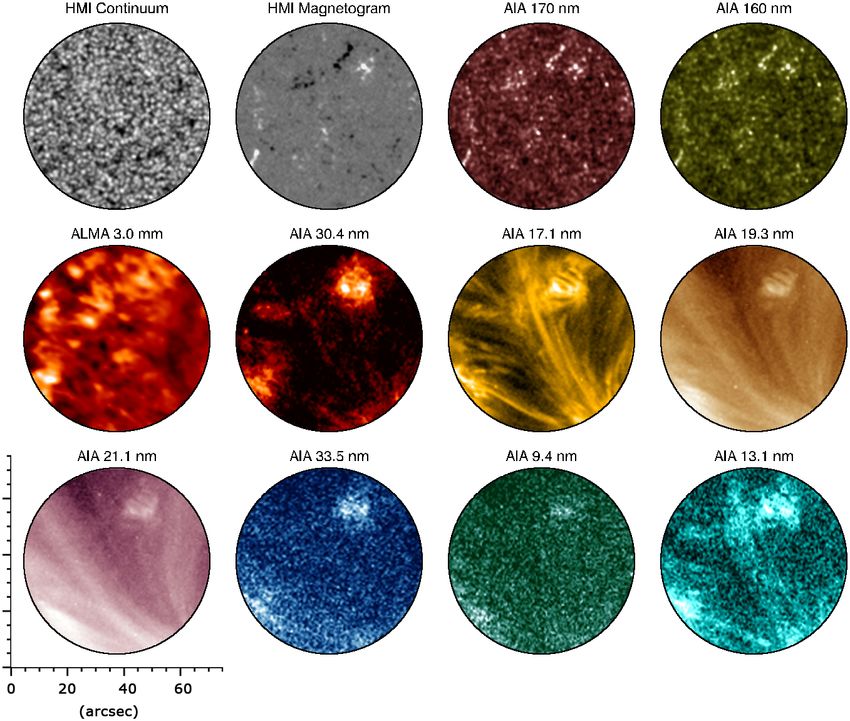
A&A 659, A31 (2022)

difficult. Due to the significant differences between solar obser-
vations and standard ALMA observations of other astronomi-
cal targets, ALMA so far delivers calibrated measurement sets
to the observers, or, more precisely, the data together with a
prepared calibration script that is to be executed by the recipi-
ent. The further processing, which includes the construction of
time series of the images, requires significant experience, time,
and resources, which has hampered access for solar physicists
who are as yet unfamiliar with millimetre data. This difficult sit-
uation initiated the development of the Solar ALMA Pipeline
(SoAP, Szydlarski et al., in prep.) with the aim of providing easy
access to science-ready solar ALMA data to the scientific com-
munity. Routine data processing with SoAP has so far resulted
in multiple science-ready imaging time series. The original data
sets were retrieved from ESO’s ALMA Science Archive (ASA1 ,
Stoehr et al. 2017) from where they can be freely downloaded
after the end of the proprietary period.
     For the publicly available sets, the calibration scripts were
executed and SoAP was applied. All resulting processed data
sets that were of sufficient quality are now made available online    Fig. 1. While scientists can always download solar measurements sets
                                                                      directly from the ALMA Science Archive, the SolarALMA project cre-
in the Solar ALMA Science Archive (SALSA), which is com-              ated an alternative, which makes access to public, science-ready data
plementary to ASA in the sense that it contains science-ready         easier. The Solar ALMA Science Archive (SALSA) is accompanied by
data (see Fig. 1).                                                    a tool library (SALAT) that also allows the exportation of SALSA data
     Here we present the first version of SALSA, consisting of 26     to a format that can be used with other analysis and visualisation tools.
such sets, the accompanying Solar ALMA Library of Auxiliary           Please see the main text for more details.
Tools (SALAT), and the first version of a header standard for the
included FITS data files. The respective single-dish TP full-disc
solar images, used for calibration, and of which all but one are      01129.S, 2016.1.01532.S, 2017.1.00653.S, 2017.1.01672.S,
also available via ASA in a ready-to-use format, are included.        2018.1.01879.S, and 2018.1.01763.S. The individual obser-
The observational data sets included in the current version of        vations target quiet-Sun and active regions for a variety of
SALSA are briefly described in Sect. 2. A brief summary of the        heliocentric angles on the solar disc. An illustrative example of
data processing with SoAP and the resulting data products are         a resulting snapshot in Band 6, close to the disc centre (from
provided in Sects. 3 and 4, respectively. SALSA and SALAT,            D22), is shown in Fig. 2.
together with guidelines for usage, documentation, and acknowl-            All time series display notable evolution for all visible fea-
edgements are addressed in Sect. 5, followed by a summary and         tures, including fibrils in some data sets. The included limb data
outlook in Sect. 6.                                                   set features a spicule or small protuberance (set labelled as D11).
                                                                      The effective angular resolution of the data sets, as set by the
                                                                      synthesised beam size, which corresponds to the primary lobe
2. Observations                                                       of a point-spread function, depends mainly on the wavelength,
Solar observations are performed using a heterogeneous array          configuration of the interferometric array, and the position of the
through the combination of the 12-m array and the ACA with            target on the sky. Consequently, the effective angular resolution
additional, typically simultaneous single-dish full-disc scans of     varies significantly between data sets and, to a lesser degree,
the Sun with several TP antennas. The data provided in the            within the individual time series due to the motion of the Sun
first version of SALSA presented here was obtained during the         across the sky, and potentially from frame to frame for various
period from December 2016 to 2018. The observations were per-         technical reasons (e.g. flagging of individual antennas).
formed in Band 3, covering the frequency range between 92                  The ALMA data sets can be aligned (spatially or temporally)
and 108 GHz, and Band 6 with frequencies between 229 and              with observations from other ground-based or space-borne tele-
249 GHz. These frequency ranges correspond roughly to an aver-        scopes (at other wavelengths) to further inspect, for example, the
age wavelength of 3 mm for Band 3 and 1.3 mm for Band 6. The          evolution of features of interest at multiple atmospheric heights
radiation in these bands is dominated by (thermal) free-free con-     and for general context. In particular, the Solar Dynamics Obser-
tinuum emission.                                                      vatory (SDO; Pesnell et al. 2012), with continuous observations
     The data sets in SALSA are labelled as Dnn (in this first        of the entire solar disc at several wavelength bands (sampling
release D01 to D28; see Table 1). We refer to these labels when       the solar photosphere, low chromosphere, transition region, and
discussing slight differences in the sets below. All released         corona), can provide complementary information to the ALMA
sets are constructed from single-pointing observations, with a        observations (these complement each other since SDO does not
12-m array and ACA, and contain time-sequences of absolute            sample the chromospheric heights captured by ALMA). Figure 3
brightness temperature maps (in units of Kelvin) at a cadence         shows an example of such alignments between an ALMA image
of 1 or 2 s. The observations cover, with some minor time             and its co-tempo-spatial images from the Helioseismic and Mag-
gaps, durations ranging from minutes to over an hour. The 26          netic Imager (HMI; Schou et al. 2012 and the Atmospheric
data sets released here are part of the following 11 success-         Imaging Assembly (AIA; Lemen et al. 2012) (onboard SDO) for
ful observational projects: 2016.1.00030.S, 2016.1.00050.S,           the first SALSA data set (i.e. D1), taken on 2016 December 22 in
2016.1.00202.S, 2016.1.00423.S, 2016.1.00572.S, 2016.1.               Band 3. All SALSA sets are provided with helioprojective coor-
                                                                      dinates, which should facilitate such alignments. However, the
1
    https://almascience.eso.org/aq/                                   given coordinates and position angles (which allow the rotation
A31, page 2 of 13
V. M. J. Henriques et al.: The Solar ALMA Science Archive (SALSA)
Table 1. All datasets present and downloadable in the initial release of SALSA.
Data Date Project ID Band/λ Cad. Obs. time (UTC) µ T mean [K] Mean resolution (a) Co- Coordinates (b) Related
[sec] bmin/bmaj [arcsec] Observations publications (c)
D01 2016-12-22 2016.1.00423.S 3/3.0 mm 2 14:19:31-15:07:07 0.99 7387 ± 519 1.37/2.10 SDO 0,0 1, 2, 3, 4, 17
D02 2017-04-22 2016.1.00050.S 3/3.0 mm 2 17:20:13-17:42:37 0.92 9317 ± 1229 1.69/2.21 IRIS,SDO −246,267 3, 4, 5, 6, 7, 15
D03 2017-04-23 2016.1.01129.S 3/3.0 mm 2 17:19:19-18:52:54 0.96 7161 ± 1564 1.92/2.30 IRIS,SDO −54,251 3, 4, 8
D04 2017-04-27 2016.1.01532.S 3/3.0 mm 2 14:19:52-15:31:17 0.78 7974 ± 1145 1.74/2.23 IRIS,SDO 520,272 3, 4
D05 2017-04-27 2016.1.00202.S 3/3.0 mm 2 16:00:30-16:43:56 0.96 7287 ± 1297 1.77/1.88 IRIS,SDO 172,−207 3, 4, 9, 10
D06 2018-04-12 2017.1.00653.S 3/3.0 mm 1 15:52:28-16:24:41 0.90 7689 ± 661 1.77/2.55 IRIS,SDO −128,−400 4, 11
D07 2017-04-18 2016.1.01129.S 6/1.3 mm 2 14:22:01-15:09:15 0.76 7167 ± 1158 0.75/2.03 IRIS,SDO −573,230 3, 4, 8
D08 2017-04-22 2016.1.00050.S 6/1.3 mm 2 15:59:17-16:43:26 0.92 7496 ± 1014 0.68/0.85 IRIS,SDO −261,266 3, 4, 5, 6, 7
D09 2018-04-12 2017.1.00653.S 6/1.3 mm 1 13:58:58-14:32:27 0.88 5700 ± 333 0.80/2.22 IRIS,SDO −175,−415 4, 11
D10 2018-08-23 2017.1.01672.S 6/1.3 mm 1 16:24:27-17:18:05 0.97 6104 ± 497 1.69/2.21 IRIS,SDO 68,−211 4
D11 2017-03-16 2016.1.00572.S 3/3.0 mm 1 15:22:33-15:32:37 0.00 7263* ± 148 2.55/4.43 SDO −679,−679 3, 11, 12, 13, 14
D12 2017-03-19 2016.1.00030.S 3/3.0 mm 2 18:16:02-19:10:13 0.86 7364 ± 302 2.52/5.06 IRIS,SDO −513,−64 –
D15 2018-08-23 2017.1.01672.S 6/1.3 mm 1 17:37:00-18:15:57 0.87 5814 ± 267 0.82/1.31 SDO 79,−238 4
D16 2017-03-16 2016.1.00572.S 3/3.0 mm 2 16:58:00-17:06:40 0.59 7768 ± 186 2.70/4.32 SDO −517,−585 3, 11, 12, 13, 14
D17 2017-03-16 2016.1.00572.S 3/3.0 mm 2 18:40:51-18:50:56 0.84 7510 ± 241 2.54/5.17 IRIS,SDO −321,−404 3, 11, 12, 13, 14
D18 2017-03-16 2016.1.00572.S 3/3.0 mm 2 17:59:04-18:09:08 0.72 7296 ± 251 2.52/4.85 SDO −468,−484 3, 11, 12, 13, 14
D19 2017-03-16 2016.1.00572.S 3/3.0 mm 2 19:23:00-19:33:05 0.91 7416 ± 234 2.46/5.77 SDO −261,−295 3, 11, 12, 13, 14
D20 2017-03-16 2016.1.00572.S 3/3.0 mm 2 16:14:48-16:24:53 0.13 4475 ± 256 2.49/4.56 SDO −686,−666 3, 11, 12, 13, 14
D21 2018-12-20 2018.1.01763.S 6/1.3 mm 1 13:19:19-14:07:32 0.38 6181 ± 208 0.60/1.05 IRIS,SDO 888,203 11
D22 2018-12-22 2018.1.01879.S 6/1.3 mm 1 15:09:14-15:14:57 1.00 6310 ± 185 0.73/1.99 SDO(d) 1, 0 −
D23 2017-04-23 2016.1.01129.S 6/1.3 mm 2 14:23:55-15:11:06 0.41 6643 ± 396 0.71/1.72 SDO −860,−129 3, 4, 8
D24 2017-03-19 2016.1.00030.S 3/3.0 mm 2 15:32:32-16:26:52 0.84 7461 ± 421 2.65/4.39 IRIS,SDO −535,−66 –
D25 2017-03-19 2016.1.00030.S 3/3.0 mm 2 16:52:52-17:47:11 0.85 7387 ± 415 2.48/4.31 IRIS,SDO −484,−46 –
D26 2018-04-12 2017.1.00653.S 3/3.0 mm 1 16:43:52-17:16:06 0.90 7553 ± 360 1.84/2.82 IRIS,SDO −131,−400 4, 11, 16
D27 2018-04-12 2017.1.00653.S 6/1.3 mm 1 14:51:20-15:25:01 0.90 5899 ± 157 0.89/2.01 IRIS,SDO 145,−400 4, 11, 16
D28 2017-03-28 2016.1.00788.S 6/1.3 mm 1 15:09:20-16:12:12 0.91 6157 ± 162 1.05/1.89 IRIS,SDO −181,347 3
Notes. The date and time of the observations, the associated project ID, receiver band, wavelength, cadence, coordinates (note that coordinates are
necessarily approximate and the accuracy depends on the set and visually identifiable features (see text)) and µ angle, mean temperature and respec-
tive standard deviation, average resolution given as the time-averaged minor and major axes of the synthesised beam, identified co-observations
by IRIS and publications where the set was used as well as publications where the same data were used but processed independently are listed.
Publications that used the sets as processed in this database as listed in bold. (a) Time average of the minor and major axes of the clean beam.
(b)
Necessarily approximate, see text (c) Publications where the SALSA set was used and publications where the data were used but processed inde-
pendently from this release. (d) DC not targeted by IRIS.
References. 1: Wedemeyer et al. (2020); 2: Eklund et al. (2020); 3: Menezes et al. (2021); 4: Jafarzadeh et al. (2021); 5: da Silva Santos et al.
(2020b); 6: Chintzoglou et al. (2021a); 7: Chintzoglou et al. (2021b); 8: Molnar et al. (2019); 9: Loukitcheva et al. (2019); 10: Martínez-Sykora
et al. (2020); 11: Alissandrakis et al. (2020); 12: Nindos et al. (2018); 13: Patsourakos et al. (2020); 14: Nindos et al. (2020); 15: Guevara Gómez
et al. (2021); 16: Nindos et al. (2021); 17: Eklund et al. (2021).
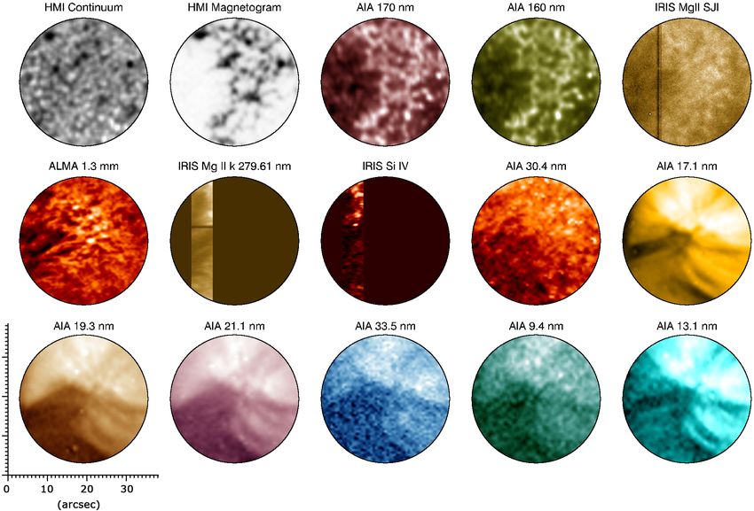
of the field of view with respect to the solar north-south direc-
tion) may be used only as a first approximation since offsets can
be expected (see Sect. 3 for details). It was found that a com-
bination of the SDO/AIA 170 nm and 30.4 nm channels (with
different brightness weights) resulted in a similar scene to that
sampled by ALMA (in both Bands 3 and 6). For Band 3, adding
the SDO/AIA 17.1 nm channel was helpful in some cases. The
combined image facilitates cross-correlations between similar
solar features with ALMA observations. The field of view illus-
trated in Fig. 3 samples a magnetically quiescent area, with small
network patches (of opposite polarities) as seen in, for exam-
ple, the HMI magnetogram and the AIA 170 and 160 nm chan-
nels. Excess brightness temperature in the ALMA image (at 3.0
mm; Band 3) over the network patches, intensity enhancements
in hotter AIA channels over some of these patches, and loops
connecting the opposite polarities, are all evident. Larger loops,
entering the field of view, are rooted in strong magnetic concen-
trations outside the target area (see e.g. Wedemeyer et al. 2020
and Jafarzadeh et al. 2021 for detailed analyses of this data set).
Another example of co-observations with other instruments
Fig. 2. Generic frame from a disc centre set (D22), showing quiet-Sun is presented in Fig. 4, where the co-spatial images from the SDO
and network features as observed in Band 6. The elliptic cross-section channels and selected images from the Interface Region Imag-
of the beam shape is plotted in the bottom left of the frame. This plot ing Spectrograph (IRIS; De Pontieu et al. 2014) explorer are
was made with SALAT (see Sect. 5.2). shown along with the ALMA Band 6 image (from 2017 April
A31, page 3 of 13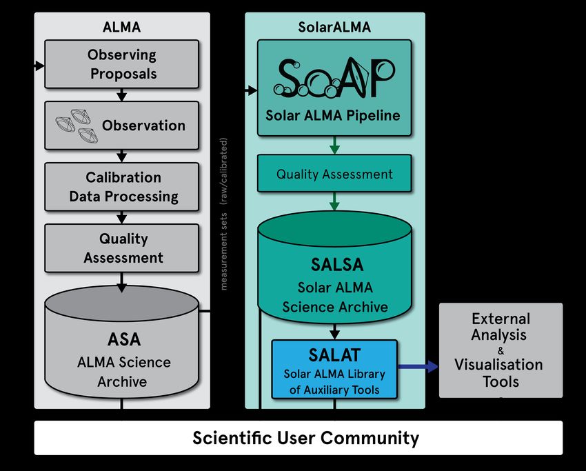
A&A 659, A31 (2022)

Fig. 3. ALMA Band 3 image from 2016 December 22 (project ID 2016.1.00423.S), along with co-aligned SDO images. Time series of images is
available online as a movie.

22; D08) at the beginning of the observations. This data set sam-    3. Data processing
ples a plage or enhanced-network region, with excess brighten-
ings above the magnetic concentrations in the ALMA image,            This first release of SALSA is the product of routine application
while chromospheric (dark) fibrillar structures (over the inter-     of the Solar ALMA Pipeline (SoAP) to the publicly released
network area) are also observed in both ALMA and IRIS Mg ii k        measurement sets available on the ALMA Science Archive
at 279.61 nm. The latter is a raster image where the slit has        (ASA, Stoehr et al. 2017). As mentioned above, the primary goal
scanned a relatively small region compared to that of ALMA.          behind SoAP is to simplify processing calibrated ALMA mea-
                                                                     surement sets into science-ready FITS imaging data. For all data
An IRIS slit-jaw image (SJI) at around the Mg ii line is also
                                                                     sets, the following steps of SoAP were executed:
shown in Fig. 4.                                                      1. Imaging including CLEAN wrapper, self-calibration (for all
    The time series of images as shown in Figs. 3 and 4 are avail-       but one data set), and primary-beam correction.
able online as a movie. We note that since the ALMA and SDO           2. Brightness temperature conversion (from Jy/beam to K).
images were taken with different cadence, the ALMA observa-           3. Bad frame discarding in time series.
tions with 2 s cadence was considered as the reference. Hence,        4. Frame-to-frame spatial alignment for ALMA time
the SDO (and IRIS) images are repeated in time to fill in the            sequences.
gaps, in a way that the time difference of the images are the         5. Combination of interferometric and total-power data.
shortest at any given time. These will result in co-alignments       The imaging part of SoAP uses the CLEAN algorithm (Högbom
of the images both temporally and spatially. It is worth not-        1974) for the deconvolution of images in the form devised by
ing that the SDO images in these two examples were resam-            Rau & Cornwell (2011) and as implemented in CASA (Common
pled to the pixel size of the ALMA images prior to the align-        Astronomy Software Applications; McMullin et al. 2007). The
                                                                     conversion from flux density to brightness temperature was done
ment, but they were not convolved with the synthesised beam
                                                                     using the Rayleigh-Jeans approximation of the Planck function
of ALMA (i.e. the corresponding PSF). For a one-to-one com-
                                                                     and the time-dependent solid angle (i.e. the area covered on the
parison, such convolutions may be necessary. Necessary rou-
                                                                     sky) of ALMA’s synthesised (elliptical cross-section) beam, fol-
tines for extracting a desired ALMA PSF and performing con-
                                                                     lowing the standard procedure2 .
volutions, along with other useful simple analyses, are provided
through the Solar ALMA Library of Auxiliary Tools (SALAT;            2
                                                                       https://science.nrao.edu/facilities/vla/proposing/
see Sect. 5.2).                                                      TBconv

A31, page 4 of 13
V. M. J. Henriques et al.: The Solar ALMA Science Archive (SALSA)
Fig. 4. Same as Fig. 3, but for ALMA Band 6 taken on 2017 April 22 (project ID 2016.1.00050.S). In addition to the SDO channels, one slit-jaw
image (SJI) and two raster images from IRIS are also displayed. Time series of images is available online as a movie.
For all sets except D01, self-calibration for phase (Cornwell ometric maps are available at a cadence of 1–2 s, while only
& Fomalont 1999) was performed. For D01, the self-calibration one or a few TP maps with many minutes in-between are usu-
method severely underperformed due to technical problems with ally available. Consequently, the lower spatial frequency scales,
pointing for those early observations. Spatial alignment (single set by the TP, will be steady, while the high spatial frequency
shift value per frame, i.e. rigid) was performed for all sets except features as set by the interferometer evolve. This would impact
the limb set to effectively correct any residual jitter and wob- the mapping of features evolving on the affected scales, with the
bling of the time series. This follows a heavily adapted version of effect becoming more severe for larger differences between the
CRISPRED’s polish tseries core routines (de la Cruz Rodríguez time at which the interferometric data was taken and the time
et al. 2015). Visually, the alignment procedure is generally suc- at which the employed TP data were recorded. For this reason,
cessful in keeping features aligned and thus maximises science save the few exceptions highlighted both here and in the meta-
potential for time evolution studies. data (see Sect. 4.1) of the data files, the combining was done by
The combining of total power and interferometric data was computing an average over 3 × 3 TP pixels at the location of the
performed in different ways as the pipeline development pro- interferometric observations and merely adding it to the inter-
gressed. The primary goal of this step is to obtain absolute ferometric data. This simpler technique avoids the introduction
brightness temperatures since the interferometer only provides of false low-spatial-frequency structures, but it reduces the low-
differences (as the zero frequency of the Fourier space would spatial-frequency information. Depending on the science case,
require a zero distance between two antennas, which cannot be this is either an advantage or a disadvantage, and a user of inter-
obtained). For D01 and D08, this combination follows a pro- ferometric data, including the one put forward in this database,
cess known as ‘feathering’, as described in Stanimirovic (2002). should be aware of the different choices made for each set. Aside
This procedure consisted of rescaling a matching TP map to the from this paper, the information on this step, can be found in
interferometric pixel scale and adding those values pixel-wise extension ‘PRPARA’ (extension 2) of each FITS data file. For
(spatially matched) to the entire cube. This technique allows for the few data sets for which no TP single-dish observations were
compensation of the incomplete uv Fourier space sampling by available, the offsets were set to the default (quiet-Sun) value,
the interferometer by adding the low-frequency spatial variation also listed in the headers, of either 7300 K for Band 3 or 5900 K
at the same time as the absolute temperature. This technique was for Band 6 as suggested by White et al. (2017). The same was
also favoured in Chintzoglou et al. (2021b) as it is desirable to done for the limb set (D11) because the TP offset setting close to
recover the low-frequency spatial scales. However, the interfer- the limb is highly uncertain. The latter is due to an overshooting
A31, page 5 of 13A&A 659, A31 (2022)
pattern present when scanning the disc with a single dish and to 4. Data products
small pointing differences leading to large changes in absolute
observed temperature. Thus, the present limb set and any future SALSA is hosted4 by the Science Data Centre at the University
releases of limb sets should only be used to study variations in of Oslo, which also, among other services, provides Hinode data.
temperature until the issue has been fixed. Each TP, as available In this section, we describe the general format and content of the
in ASA, is itself calibrated by assuming that the average bright- data products and the selection of data sets provided in the first
ness temperature in a region around disc centre has a value of release of SALSA.
7300 K for Band 3 or 5900 K for Band 6, again following White
et al. (2017). We note that this is not the same as setting the total 4.1. Data format and header standard
power of an interferometric time series calibrated with that map
to this same value. The TP signal is impacted by any bright or The ALMA data on SALSA is provided as flexible image trans-
dark features in the region targeted by the interferometric array port system (FITS) files containing the brightness temperatures
and also beyond corresponding to the beam pattern. Even if there as five-dimensional data arrays (in units of Kelvin) and two
is a significant time difference between the TP scan and the inter- extensions. The first two array dimensions are the usual spatial
ferometric observations, the activity levels and heliocentric angle dimensions, the third is wavelength, the fourth is Stokes, and the
alone will result in the offset extracted from the TP being differ- fifth is time. This format was chosen in preparation for future
ent than the quiet-Sun disc-centre value. Significant limb bright- data sets that will make use of all five dimensions, even though
ening (10% for Band 3 and 15% for Band 6) was found at these the data sets in this first release consist of continuum time series
wavelengths and specific bandpasses (Alissandrakis et al. 2017; only (one wavelength, one Stokes component). The extension
Sudar et al. 2019) and is thus a contributing factor, captured via ‘TIMEVAR’ contains a binary table with time-variable infor-
TP calibration, to the final observed brightness temperature of mation. The table is self-described in the headers of the exten-
the released sets. sion and will be extended in future releases. At the time of this
Multiple scans, that is, continuous observing periods, were release, it consists of the beam properties and time tags for each
combined whenever possible provided the target is the same and frame present in the cube. The first element of the table is the
the time difference between scans is small. Because small time major axis of ellipse used to describe the beam, the second the
gaps are present between scans, the user should use the time minor axis, the third is the beam position angle, and the fourth
stamps per frame when doing any time-dependent analysis to the time tag. Following Rots et al. (2015), the time tags are pre-
avoid any such gaps or otherwise missing frames (e.g. filtered- sented in seconds counting from DATEREF (not to be confused
out bad frames) within the series. with REF_TIME), here set to the midnight at the start of the
A final step to further reduce high frequency noise consisted date of the observations (i.e. 00:00:00.000). These beam prop-
of smoothing in time. The smoothing function and size are listed erties can be used to compute a proxy for angular resolution by
in the FITS metadata. For this release, most sets received a final taking the mean of the minor and major axes, and such infor-
smoothing with a boxcar of five frames (so 5-to-10-s smooth- mation is provided in the headers under the ALMA keyword
ing depending on the set cadence). This smoothing was found SPATRES. For this database, SPATRES varies from 0.77 arc-
to be important to be able to release all time series at the high- sec to 4.11 arcsec. The time-dependent beam properties from
est cadence possible, but ongoing refinements may make such the extension TIMEVAR should be considered for wave studies
filtering obsolete for most sets added or revised in the future. where very small scales are analysed.
Coordinates of the observations are computed using the RA The second extension, PRPARA, contains an ASCII table
and DEC listed in each measurement set released by the ASA with parameter names, values, and descriptions for different pro-
and the ‘reference time’, which is usually the time of the first cessing steps. The processing steps are named in the header of
solar pointing (first same-named source for the first science the extension and also in the primary header of the file using
scan in the case of multiple solar targets). These measurement SOLARNET’s ‘detailed description of all processing steps’
set coordinates are converted to helioprojective Cartesian (X,Y) formalism (Sect. 8.2 thereof) which can be identified by the
coordinates in arcseconds by using the solar disc centre RA and PRXXXn keywords. These include information on the used ver-
DEC at the reference time. SoAP includes a routine for such sions of CASA, SoAP, and other relevant details concerning data
conversions, but, for some data sets in this first release, the web processing. Together with the public release of SoAP, which
interface of the ALMA Solar Ephemeris Generator (Skokić & is planned for the near future, this allows advanced users to
Brajša 2019)3 was used. The helioprojective coordinates, the ref- not only reproduce the data but also potentially optimise the
erence time, and other useful coordinate information such as the data reduction towards wanted properties; for example, priori-
‘P’ angle (i.e. position angle of the solar north pole) are listed tising brightness temperature over accurate reproduction of spa-
in the headers of each data file under the World Coordinate Sys- tial structure. Further details on the headers and extensions is
tem A (see Appendix A). Due to pointing issues in the early provided in the Appendices A and B. The files are compliant
cycles, a target-dependent error of up to 20 arcsec is expected to with the Flexible Image Transport System NASA standard ver-
be present (private communication). The pointing accuracy was sion 3.0, 4.0, with the evolving ALMA header format standard
improved for sets where co-simultaneous observations (e.g. with (Felix Stoehr, priv. comm.), and the SOLARNET Metadata Rec-
SDO) allowed for a refinement of the actually observed coordi- ommendations document version 1.4 (Haugan & Fredvik 2020).
nates. The listed coordinates are the corrected values whenever
possible, but in principle, they should be taken with caution due 4.2. Data sets in the first SALSA release
to the possibility of persisting multi-arcsec offsets from actual
coordinates. All data sets that are included in the first release of SALSA
are listed in Table 1. They all contain time series of contin-
uum brightness temperature maps. Please note that data sets
3 4
https://celestialscenes.com/alma/convert/ http://sdc.uio.no/salsa/
A31, page 6 of 13V. M. J. Henriques et al.: The Solar ALMA Science Archive (SALSA)
for (quasi-static) mosaics can be retrieved directly from the 5.2. SALAT
ASA. For the data sets on SALSA, fundamental information
such as date, band, helioprojective coordinates at the start of the The Solar ALMA Library of Auxiliary Tools (SALAT5 ) enables
time series, and identified co-observations are listed. In the first easy loading and initial visualisation and exploration of SALSA
release, mostly co-observations with IRIS are considered as it is data products in both Interactive Data Language (IDL) and
a highly complementary observatory, providing sampling of the Python. For a complete description of SALAT, installation guide
transition region and chromosphere in high spectral resolution. and examples, please visit the corresponding webpage7 . SALAT
Attempts by multiple observatories to coordinate with ALMA includes routines (IDL) and functions (Python) for reading the
were made but not necessarily guaranteed or successful due to FITS files and extracting useful information such as arrays with
the common challenges of observations such as accurate point- the observing times or the synthesised beam shape for each
ing and timing. This was also the case for a few observations ALMA image frame. It can be used to compute basic statistics
coordinated with IRIS that we found to not have overlapping for the time-series or individual frames, as well as for the cor-
target regions on the Sun. For example, for D22 the disc centre responding ALMA synthesised beam, which are all important
was observed by ALMA, which was not the coordinated target for advanced analysis. Functions to plot ALMA data, includ-
observed by IRIS. For D11, D16, D18, and D19, the correct tar- ing the beam shape, and the possibility of saving the images
gets were observed by IRIS but not at the same time as ALMA. are included. SALAT can also be used for identifying the best
A direct link to the specific IRIS observations page is provided frames in an observation or to obtain a general idea of the time-
on SALSA’s web interface, which typically includes informa- line during the observation period, including any time gaps due
tion on further observatories, including SDO and Hinode. The to filtered-out frames or concatenated scan periods. Useful for
SALSA web-interface also provides the corresponding full-disc the production of synthetic observables and comparison with
TP map of the Sun on which the location of the interferometri- co-observations, SALAT allows the usage of the ALMA beam
cally observed region is marked. These are the TP maps used for of a particular observation to convolve it with other types of
calibration (multiple TP observations may exist per set). Such data, such as complementary data sets and simulations. Finally,
TPs are available from ASA, but are reproduced in SALSA for SALAT can be used to create a new FITS file with the appro-
convenience and record completeness. As an exception, being priate format (e.g. reduced dimensions), which can be inspected
an early set, D01’s TP is only available in raw format at ASA with other external viewing or analysis tools such as SAOIm-
but was processed in the same way as the remaining TPs for the ageDS9 (Joye & Mandel 2003), CARTA (Comrie et al. 2021),
production of D01 (described in Sect. 3). It is available as a final CRISPEX (Vissers 2012; Löfdahl et al. 2021), and so on.
product at SALSA.
Some sets from SALSA have been reduced by other 6. Summary and outlook
researchers independently of this database and were used in
diverse publications. The reductions are not always comparable. We present the first release of SALSA – a database of 26 science-
A main point of difference is that we only release sets at high ready data sets for ALMA observations of the Sun. We also
cadence, and other publications might consider averaged proper- present the first release of SALAT, an IDL and Python package
ties. The last column of Table 1 identifies all publications known for loading and initial visualisation and exploration of SALSA
to have used the same raw data (but with different processing) data products. We plan to extend SALSA with additional data
and publications for which sets from this database were used. sets in the future. Depending on the further development of solar
The latter are marked in bold. observing modes with ALMA, new data sets for new capabili-
ties will be added. That includes, for instance, data measured in
other receiver bands (e.g. Band 5 or 7), different frequency setup
(e.g. sub-band sampling), mosaics, other antenna array configu-
5. Obtaining and using SALSA data rations, but also different image reconstruction techniques.
5.1. SALSA
Acknowledgements. We kindly ask to add the following acknowledgement
The data files in FITS format can be downloaded from SALSA5 to any publication that uses data downloaded from SALSA: “This paper
by accessing the webpage6 and clicking ‘download’ in the appro- makes use of the following ALMA data: [ALMA-PROJECT-ID] . ALMA
is a partnership of ESO (representing its member states), NSF (USA) and
priate column for each of the desired sets. Sets can be selected NINS (Japan),together with NRC(Canada), MOST and ASIAA (Taiwan),
using their listed properties, either manually or by using the and KASI (Republic of Korea), in co-operation with the Republic of Chile.
search bar on the top right of the table, by the quality and visible The Joint ALMA Observatory is operated by ESO, AUI/NRAO and NAOJ.
structures upon examination of the playable embedded movie SALSA, SALAT and SoAP are produced and maintained by the SolarALMA
(press ‘movie’ button), or by the location on the solar disc and project, which has received funding from the European Research Council
(ERC) under the European Union’s Horizon 2020 research and innovation
respective context, as identifiable by the square marker overlaid programme (grant agreement No. 682462), and by the Research Council of
on the image of the TP single-dish scan shown in the last col- Norway through its Centres of Excellence scheme, project number 262622.”
umn. The latter corresponds to the TP map used for total power The ALMA-PROJECT-ID can be found in the FITS header keyword PROJID of
calibration, as described in Sect. 3. The data arrays are ready to the SALSA data file, e.g. ADS/JAO.ALMA#2016.1.00423.S. Optionally, we are
open for collaboration on science projects in the form of technical support or
use in a form analogous to any other solar data, and they fol- help with scientific analysis and co-authorship of resulting publications. Please
low the format described in Sect. 4. The headers and extensions refer to the SALSA webpage (http://sdc.uio.no/salsa/) for more infor-
provide additional advanced information following the standard mation or contact us directly (e-mail address: Psolaralma@astro.uio.no.).
described in Appendices A and B. This work is supported by the SolarALMA project, which has received
funding from the European Research Council (ERC) under the European
Union’s Horizon 2020 research and innovation programme (grant agree-
ment No. 682462), and by the Research Council of Norway through its
5
Please send requests for technical support or scientific collaboration Centres of Excellence scheme, project number 262622. This paper makes
to the following e-mail address: solaralma@astro.uio.no.
6 7
http://sdc.uio.no/salsa/ https://solaralma.github.io/SALAT/
A31, page 7 of 13A&A 659, A31 (2022)
use of the following ALMA data: ADS/JAO.ALMA#2016.1.00030.S, Guevara Gómez, J. C., Jafarzadeh, S., Wedemeyer, S., et al. 2021, Phil. Trans. R.
ADS/JAO.ALMA#2016.1.00050.S, ADS/JAO.ALMA#2016.1.00202.S, ADS/ Soc. London Ser. A, 379, 20200184
JAO.ALMA#2016.1.00423.S, ADS/JAO.ALMA#2016.1.00572.S, ADS/JAO. Haugan, S. V. H., & Fredvik, T. 2020, https://doi.org/10.5281/zenodo.
ALMA#2016.1.01129.S, ADS/JAO.ALMA#2016.1.01532.S, ADS/JAO.AL 5719255
MA#2017.1.00653.S, ADS/JAO.ALMA#2017.1.01672.S, ADS/JAO.ALMA Högbom, J. A. 1974, A&AS, 15, 417
#2018.1.01879.S, and ADS/JAO.ALMA#2018.1.01763.S. ALMA is a partner- Jafarzadeh, S., Wedemeyer, S., Szydlarski, M., et al. 2019, A&A, 622, A150
ship of ESO (representing its member states), NSF (USA) and NINS (Japan), Jafarzadeh, S., Wedemeyer, S., Fleck, B., et al. 2021. Phil.Trans. R. Soc. London
together with NRC(Canada), MOST and ASIAA (Taiwan), and KASI (Republic Ser. A, 379, 20200174
of Korea), in co-operation with the Republic of Chile. The Joint ALMA Joye, W. A., & Mandel, E. 2003, in Astronomical Data Analysis Software and
Observatory is operated by ESO, AUI/NRAO and NAOJ. We are grateful to the Systems XII, eds. H. E. Payne, R. I. Jedrzejewski, & R. N. Hook, ASP Conf.
many colleagues who contributed to developing the solar observing modes for Ser., 295, 489
ALMA, including the international ALMA solar development group and the Karlický, M., Bárta, M., Dabrowski,
˛ B. P., & Heinzel, P. 2011, Sol. Phys., 268,
participants of the First International Workshop on Solar Imaging with ALMA 165
(ALMA-SOL-IMG1), and for support from the ALMA Regional Centres. We Lemen, J. R., Title, A. M., Akin, D. J., et al. 2012, Sol. Phys., 275, 17
are indebted to the ALMA Science Archive team for their excellent product Löfdahl, M. G., Hillberg, T., de la Cruz Rodríguez, J., et al. 2021, A&A, 653,
and to Felix Stoehr in particular for comments on the FITS header standard. A68
We thank Pit Sütterlin for his excellent code contributions throughout the years Loukitcheva, M. A., Solanki, S. K., & White, S. 2008, Ap&SS, 313, 197
which we continuously come back to when building new infrastructure such as Loukitcheva, M. A., White, S. M., & Solanki, S. K. 2019, ApJ, 877, L26
image alignment and scaling optimisation routines. Rob Rutten’s public SDO Martínez-Sykora, J., De Pontieu, B., de la Cruz Rodriguez, J., & Chintzoglou,
alignment routines were used for the figure examples. We thank Terje Fredvik G. 2020, ApJ, 891, L8
for valuable comments on the final header products, which helped us follow McMullin, J. P., Waters, B., Schiebel, D., Young, W., & Golap, K. 2007, in
the recommendations from SOLARNET, an European Union’s Horizon 2020 Astronomical Data Analysis Software and Systems XVI, eds. R. A. Shaw,
research and innovation programme under grant agreement No. 824135. Finally, F. Hill, & D. J. Bell, ASP Conf. Ser., 376, 127
we thank Stian Aannerud for the final testing of SALSA and SALAT. Menezes, F., Selhorst, C. L., Giménez de Castro, C. G., & Valio, A. 2021, ApJ,
910, 77
Molnar, M. E., Reardon, K. P., Chai, Y., et al. 2019, ApJ, 881, 99
References Nindos, A., Alissandrakis, C. E., Bastian, T. S., et al. 2018, A&A, 619, L6
Nindos, A., Alissandrakis, C. E., Patsourakos, S., & Bastian, T. S. 2020, A&A,
Alissandrakis, C. E., Patsourakos, S., Nindos, A., & Bastian, T. S. 2017, A&A, 638, A62
605, A78 Nindos, A., Patsourakos, S., Alissandrakis, C. E., & Bastian, T. S. 2021, A&A,
Alissandrakis, C. E., Nindos, A., Bastian, T. S., & Patsourakos, S. 2020, A&A, 652, A92
640, A57 Patsourakos, S., Alissandrakis, C. E., Nindos, A., & Bastian, T. S. 2020, A&A,
Bastian, T. S. 2002, Astron. Nachr., 323, 271 634, A86
Bastian, T. S., Chintzoglou, G., De Pontieu, B., et al. 2017, ApJ, 845, L19 Pesnell, W. D., Thompson, B. J., & Chamberlin, P. C. 2012, Sol. Phys., 275, 3
Bastian, T. S., Bárta, M., Brajša, R., et al. 2018, The Messenger, 171, 25 Rau, U., & Cornwell, T. J. 2011, A&A, 532, A71
Brajša, R., Sudar, D., Benz, A. O., et al. 2018, A&A, 613, A17 Rodger, A. S., Labrosse, N., Wedemeyer, S., et al. 2019, ApJ, 875, 163
Brajša, R., Skokić, I., Sudar, D., et al. 2021, A&A, 651, A6 Rots, A. H., Bunclark, P. S., Calabretta, M. R., et al. 2015, A&A, 574, A36
Chintzoglou, G., De Pontieu, B., Martínez-Sykora, J., et al. 2021a, ApJ, 906, Schou, J., Scherrer, P. H., Bush, R. I., et al. 2012, Sol. Phys., 275, 229
82 Selhorst, C. L., Simões, P. J. A., Brajša, R., et al. 2019, ApJ, 871, 45
Chintzoglou, G., De Pontieu, B., Martínez-Sykora, J., et al. 2021b, ApJ, 906, Shimojo, M., Bastian, T. S., Hales, A. S., et al. 2017a, Sol. Phys., 292, 87
83 Shimojo, M., Hudson, H. S., White, S. M., Bastian, T. S., & Iwai, K. 2017b, ApJ,
Comrie, A., Wang, K. S., Hsu, S. C., et al. 2021, CARTA: The Cube Analysis 841, L5
and Rendering Tool for Astronomy Skokić, I., & Brajša, R. 2019, Rudarsko-geološko-naftni zbornik, 34, 59
Cornwell, T., & Fomalont, E. B. 1999, in Synthesis Imaging in Radio Astronomy Stanimirovic, S. 2002, in Single-Dish Radio Astronomy: Techniques and
II, eds. G. B. Taylor, C. L. Carilli, & R. A. Perley, ASP Conf. Ser., 180, 187 Applications, eds. S. Stanimirovic, D. Altschuler, P. Goldsmith, & C. Salter,
da Silva Santos, J. M., de la Cruz Rodríguez, J., White, S. M., et al. 2020a, A&A, ASP Conf. Ser., 278, 375
643, A41 Stoehr, F., Manning, A., Moins, C., et al. 2017, The Messenger, 167, 2
da Silva Santos, J. M., de la Cruz Rodríguez, J., Leenaarts, J., et al. 2020b, A&A, Sudar, D., Brajša, R., Skokić, I., & Benz, A. O. 2019, Sol. Phys., 294, 163
634, A56 Thompson, W. T. 2006, A&A, 449, 791
de la Cruz Rodríguez, J., Löfdahl, M. G., Sütterlin, P., & Hillberg, T. 2015, & Valle Silva, J. F., Giménez de Castro, C. G., Selhorst, C. L., Raulin, J. P., & Valio,
Rouppe van der Voort. L., A&A, 573, A40 A. 2021, MNRAS, 500, 1964
De Pontieu, B., Title, A. M., Lemen, J. R., et al. 2014, Sol. Phys., 289, 2733 Vissers, G., & Rouppe van der Voort, L. 2012, ApJ, 750, 22
Dulk, G. A. 1985, ARA&A, 23, 169 Wedemeyer, S., Bastian, T., Brajša, R., et al. 2016, Space Sci. Rev., 200, 1
Eklund, H., Wedemeyer, S., Szydlarski, M., Jafarzadeh, S., & Guevara Gómez, Wedemeyer, S., Szydlarski, M., Jafarzadeh, S., et al. 2020, A&A, 635, A71
J. C. 2020, A&A, 644, A152 White, S. M., Loukitcheva, M., & Solanki, S. K. 2006, A&A, 456, 697
Eklund, H., Wedemeyer, S., Szydlarski, M., & Jafarzadeh, S. 2021, A&A, 656, White, S. M., Iwai, K., Phillips, N. M., et al. 2017, Sol. Phys., 292, 88
A68 Wootten, A., & Thompson, A. R. 2009, IEEE Proc., 97, 1463
Greisen, E. W., & Calabretta, M. R. 2002, A&A, 395, 1061 Yokoyama, T., Shimojo, M., Okamoto, T. J., & Iijima, H. 2018, ApJ, 863, 96
A31, page 8 of 13V. M. J. Henriques et al.: The Solar ALMA Science Archive (SALSA)
Appendix A: Data file headers the description of each keyword, we include the list of stan-
dards that constrain or originated its usage. These are abbrevi-
The header keywords in the SALSA FITS files seek to ensure ated in the following way: F3.0 for NASA FITS Standard 3.0
reproducibility of the data, facilitate easy search across the (sometimes preferred in CASA documentation), F4.0 for NASA
archive for data fulfilling specific criteria, and ensure the avail- FITS Standard 4.0, T2006 for Thompson (2006), SNET for the
ability of critical metadata information in a standardised fashion SOLARNET recommendations document, S1.9 for the ALMA
that respects all the previous conventions. We specifically guar- FITS data-product standard version 1.9, and A611 or A613 for
antee that the SALSA data format conforms to the FITS standard ALMA memos 611 and 613, respectively.
3.0 and 4.0, the SOLARNET recommendations (under revision: World Coordinate System keywords are used according to
Haugan & Fredvik 2020), representation of World Coordinates Greisen & Calabretta (2002) and Thompson (2006) to describe
in FITS (Greisen & Calabretta 2002), World Coordinate System the data coordinates in two separate coordinate systems. The pri-
for Solar Observations (following Thompson 2006), and Rots mary coordinate system specifies RA/DEC in a SIN projection,
et al. (2015) for time-coordinate representation in FITS files. The and thus CTYPE1=’RA—SIN’ and CTYPE2=’DEC–SIN’. The
most recent evolving ALMA FITS data-product standard (Felix secondary coordinate system specifies helioprojective longitude
Stoehr, private communication) and ALMA memo 611 were also and latitude in a gnomonic projection, and thus CTYPE1A =
followed with slight departures from the memo where a collision ’HPLN-TAN’ and CTYPE2A = ’HPLT-TAN’ (note suffix A in
was present. ALMA memo 613 was also used to inform deci- keyword names for the secondary system).
sions where two options were possible. Adaptation of existing The existing CASA keywords were passed through at this
keywords was necessary but kept to a minimum and never went stage unless they were set to be changed as per the most recent
against any standards. Three headers exist, one per HDU, with information regarding the ALMA FITS data-product standard.
relevant keywords per extension. An example of this is the keyword ORIGIN, set in most archival
The keywords are listed, per extension, in Tables A.1 and data to be the CASA version where it should instead display the
B.1, with an example and a short description. The heliopro- originating institution (in agreement with FS3.0 and FS4.0). In
jective coordinates keywords are summarised in Table A.2. In such cases, the header in SALSA data files is corrected.
Table A.1. Keywords used in all SALSA data products and respective description with examples.
Generic FITS keywords common for all SALSA data products
Keyword Example Value Description
PROPCODE ’2018.1.01879.S’ Project code to which the data belongs. String. Set by
S.19.
PROJECT ’SolarALMA’ Project. String. Set by SNET.
INSTRUME ’BAND3’ Band. String. Reserved by FS3.0. FS4.0. Set by S1.9.
FILENAME ’solaralma.....image.fits’ Filename. String. Set by SNET.
DATAMIN 5800 Minimum value of the data. Float. Reserved and set by:
F3.0, F4.0, SNET.
DATAMAX 6100 Maximum value of the data. Float. Reserved and set by:
F3.0, F4.0, SNET.
CASAVER ’CASA 3.4.0(release r19988)’ String. Set by S1.9 and A613.
ORIGIN ’JAO-UIO’ UIO appended. String. Reserved by F3.0. F4.0. Set by
S1.9.
SOLARNET ’0.5’ 0.5 or 1 for partially compliant or fully compliant. String.
Set by SNET
PWV 0.7 Unit: mm. Average precipitable water vapour. Float. A
quality metric.
SPATRES 0.5 Geometric average of the min and the max beam axes (a
sort of "Spatial resolution"). Float. Arcsec. Set by A613
and S1.9.
BNDCTR 2.315424966698E+11 Center frequency of data in the FITS array. Hz. Set by
S1.9 and SNET.
WAVEBAND ’ALMA Band 3’ Human readable band description. SNET.
OBS_HDU 1 Contains Observational data. Integer. Set by SNET.
DATE-BEG ’2014-12-11T19:09:13’ Start of solar observations. String. Set by FS3.0 ,FS4.0,
SNET.
DATATAG ’This paper makes use of the following ALMA data: Set by S1.9. Implemented in SALSA as an OGIP 1.0
ADS/JAO.ALMA# [Project code]. ALMA is a partnership of compliant LONGSTRN.
ESO (representing its member states), NSF (USA) and NINS
(Japan), together with NRC (Canada) and NSC and ASIAA
(Taiwan), in cooperation with the Republic of Chile. The Joint
ALMA Observatory is operated by ESO, AUI/NRAO and NAOJ.
It also makes use of the Solar ALMA Science Archive developed
at UiO and based on SoAP reduction. Please cite ...’
A31, page 9 of 13A&A 659, A31 (2022)
Table A.1. continued.
Primary HDU FITS keywords
Keyword Default Value Description
CREATOR ’SoAP’ Name of the last software that created the data contents.
String. Set by SNET.
VERS_SW ’0.12’ Version of the CREATOR software. String. Set by SNET.
HASH_SW ’424d417e04...’ Hash of CREATOR software (robust versioning). Can be
GIT hub commit hash. Example is the hash for the latest
version marked as v0.14. String. Making its way into SNET.
CO_OBS ’IRIS 3640009423,SST,NST’ Comma separate list of telescopes with identified co-
observations and strings of observation IDs if available.
String.
CHNRMS 0.324E-03 Channel RMS. Kelvin. Float. Set by S1.9 and A613 (but not
in Jy/beam).
FOV 1.54 Total area of the field of view of the image. Square degrees.
Float. Set by S1.9.
EFFDIAM 0.70 Effective diameter of the field of view. Degrees. Float. Set
by S1.9
RES_MEAN 0.1 Mean of residuals after CLEAN. Float. Basic quality mea-
sure.
RES_STDV 0.1 Standard deviation of the residuals. Float. Basic quality mea-
sure.
VAR_KEYS ’TIMEVAR; BMAJ, BMIN, BPA, TIME_TAG’ Reference to extension containing time-variable values.
String. Set by SNET.
PRSTEP1 ’CLEAN’ Processing steptype. Generic form is PRSTEPn where n
stands for number of processing step. String. Set by SNET.
PRPROC1 ’TCLEAN’ Name of procedure performing PRSTEP1. String. Set by
SNET.
PRPVER1 0.8 Version of procedure PRPROC1. String. Set by SNET.
PRREF1A ’UIO-ALMA (solaralma@uio.no)’ Group doing manual adjustments. String. Set by SNET.
PRPARA1 ’[PRPARA]’ Name of extension containing list of parameters or options
for PRPROC1. String. Set by SNET.
PRLIB1 ’CASA ’ Software library containing TCLEAN. String. Set by SNET.
PRVER1 5.6 Library version or Modified Julian Day (MJD) of last update.
String. Set by SNET.
PRSTEP2 ’TPCALIB’ PRocessing steptype. Generic form is PRSTEPn where n
stands for number of processing step. Set by SNET.
PRPROC2 ’SOAP_FEATHER’ Name of procedure performing PRSTEP1. String. Set by
SNET.
PRPVER2 1.0 Version of procedure PRPROC2. String. Set by SNET.
PRPARA2 ’[PRPARA]’ Name of extension containing list of parameters or options
for PRPROC2. String. Set by SNET.
A31, page 10 of 13V. M. J. Henriques et al.: The Solar ALMA Science Archive (SALSA)
Table A.2. World coordinate system keywords for solar imaging data used in SALSA. Generic keywords.
World Coordinate System - Helioprojective keywords
Keyword Default Value Description
WCSNAMEA ’Helioprojective-cartesian’ Name of coordinate set. String. Set by T2006 and A611.
CTYPE1A ’HPLN-TAN’ Axis labels. Set by T2006 and A611.
CTYPE2A ’HPLT-TAN’ Axis labels. Set by T2006 and A611.
CRPIX1A 180.5 Reference pixel: center of image in pixels. Set by T2006 .
CRPIX2A 180.5 Reference pixel: center of image in pixels. Set by T2006.
CUNIT1A ’arcsec’ Angles in arcsec. Set by T2006 and A611. Arcsec is allowed by WCS.
CUNIT2A ’arcsec’ Angles in arcsec. Set by T2006 and A611. Arcsec is allowed by WCS.
CDELT1A 0.55 Plate scale (i.e. pixel size). Set by T2006. Here in arcsec as in A611.
CDELT2A 0.55 Plate scale (i.e. pizel size). Set by T2006. Here in arcsec as in A611.
CRVAL1A 0.0 Helioprojective x (solar x) coordinate of the reference pixel in arcsec.
Set by T2006. Here in arcsec as in A611.
CRVAL2A 0.0 Helioprojective y (solar y) coordinate of the reference pixel in arcsec.
Set by T2006. Here in arcsec as in A611.
CTYPE5 ’TIME’ This is in relation to REF_TIME, per frame. Time found in TIME_TAG
under extension TIMEVAR.
CUNIT5 ’s’ Unit for fifth axis. Seconds in relation to REF_TIME, per frame. Time
found in TIME_TAG under extension TIMEVAR. Normally preceding
midnight.
DSUN_OBS 147296035413.001 Distance between observer and Sun in meters. Set by T2006 and A611
with A611 precision.
RSUN_REF 696000000.0 Radius of the Sun in meters. Set by T2006 and A611 with A611 preci-
sion.
RSUN_OBS 6.96e8 Observed radius of the Sun in arcsec. Set by T2006 and A611 with tabled
A611 precision.
HGLN_OBS 0 Heliographic longitude of the observer, in degrees. Set by T2006 and
A611.
HGLT_OBS −0.47 Stonyhurst heliographic latitude of the observer, in degrees (in this coor-
dinate set identical to the classical “B0 ”). Set by T2006 and A611.
SOLAR_P 11.6872 Degrees. "rotate image by -solar P angle to get solar north up". Set by
A611.
SOLAR_P0 11.6872 Degrees. "rotate image by -solar P angle to get solar north up". Set by
SNET.
REF_TIME 2014-12-11T19:09:13 Date and time. Time used for coordinate calculations. Set by A611. Note
that, in the ASA scripts, this is typically “refTime”, without the under-
score.
A31, page 11 of 13A&A 659, A31 (2022)
Appendix B: Extension data example of such an ASCII table from a specific file. The format
is compatible with F3.0 and F4.0, and is included for the goal
We used extensions for technical details regarding data reduction of reproducibility. The main header merely refers to that exten-
and time-varying information. The extension ‘TIMEVAR’ con- sion by its name in square brackets in the PRPARAnn keyword,
tains time-varying information stored in a standard binary table as defined in the SOLARNET recommendations (described in
format. It follows the variable-keyword mechanism described in Section 8.2 of the version currently under revision). The main
Appendix I-d of the SOLARNET recommendations. It can be header PRSTEPn keyword is used to specify the main methods
selected programmatically by name (EXTNAME = ’TIMEVAR’) used, for which the parameters in this ASCII table will be rele-
and is referenced in the main header through the VAR_KEYS vant. Table B.2 lists an example of a header of an extension con-
keyword. Its parameters are listed in Table B.1. These are the taining such processing parameters. We note that these include
beam shape parameters BMAJ, BMIN, and BPA as functions a repetition of the PRxxxx keywords as also suggested by the
of time and the time stamps (TIME_TAG) of each frame of the SOLARNET recommendations. In the example printed out, the
primary HDU. The TIME_TAG values are expressed in seconds first 17 rows are spelled as in the CASA tclean routine call, as
from DATEREF following Rots et al. (2015). made by SoAP, and are recognisable in the general context of the
The second extension, ‘PRPARA’, contains parameters that CLEAN algorithm (the headers PRSTEP1). The remaining rows
might change by data set for each processing step, stored as an refer to other SoAP post-processing steps using native functions
ASCII table for readability. Code box B.3 presents a printout (the headers PRSTEP2).
Table B.1. Header of the extension with time-dependent variables, extension ‘TIMEVAR’, with example values. We note that the header keywords
describe the variables in the binary table.
Header of the extension containing time dependent variables.
Keyword Default Value Description
XTENSION ’BINTABLE’ Type of extension. String. Set by F4.0.
TFIELDS 4 Total fields. Integer. Set by F4.0.
EXTNAME ’TIMEVAR’ Name of the extension. String. Primary HDU refers to this name using
VAR_KEYS
DATEREF ’2014-12-11T00:00:00’ Time in UTC. Reference time that sets the zero to all other UTC times
such as the extension time stamps. String. Set by SNET and F4.0.
SOLARNET 0.5 SOLARNET compliance: 0.5 or 1 for partially compliant or fully com-
pliant. Float. Set by SNET.
TTYPE1 ’BMAJ’ First column. Beam shape major axis. Variable-keyword. String.
Degrees. Set by F4.0.
TTYPE2 ’BMIN’ Second column. Beam shape minor axis. Variable-keyword. String.
Degrees. Set by F4.0.
TTYPE3 ’BPA’ Third column. Beam average. Variable-keyword. String. Degrees. Set by
F4.0.
TTYPE4 ’TIME_TAG’ Fourth column. Tabulation of time. Variable-keyword. String. Set by
F4.0.
TFORM1 ’1558E’ Real*4 (float). String. Set by F4.0 and SNET.
TFORM2 ’1558E’ Real*4 (float). String. Set by F4.0 and SNET.
TFORM3 ’1558E’ Real*4 (float). String. Set by F4.0 and SNET.
TFORM4 ’1558E’ Real*4 (float). String. Set by F4.0 and SNET.
TDIM1 ’(1,1,1,1,1558)’ Dimension of array. String. Set by F4.0 and SNET.
TDIM2 ’(1,1,1,1,1558)’ Dimension of array. String. Set by F4.0 and SNET.
TDIM3 ’(1,1,1,1,1558)’ Dimension of array. String. Set by F4.0 and SNET.
TDIM4 ’(1,1,1,1,1558)’ Dimension of array. String. Set by F4.0 and SNET.
TUNIT1 ’arcsec’ Units for column 1. String. Set by F4.0 and SNET.
TUNIT2 ’arcsec’ Units for column 2. String. Set by F4.0 and SNET.
TUNIT3 ’arcsec’ Units for column 3. String. Set by F4.0 and SNET.
TUNIT4 ’s’ Units for column 4. String. Set by F4.0 and SNET.
A31, page 12 of 13You can also read