The Mediterranean climate change hotspot in the CMIP5 and CMIP6 projections
←
→
Page content transcription
If your browser does not render page correctly, please read the page content below
Research article
Earth Syst. Dynam., 13, 321–340, 2022
https://doi.org/10.5194/esd-13-321-2022
© Author(s) 2022. This work is distributed under
the Creative Commons Attribution 4.0 License.

                     The Mediterranean climate change hotspot
                        in the CMIP5 and CMIP6 projections
       Josep Cos1 , Francisco Doblas-Reyes1,2 , Martin Jury1,3 , Raül Marcos1 , Pierre-Antoine Bretonnière1 , and
                                                  Margarida Samsó1
                   1 EarthSciences Department, Barcelona Supercomputing Center (BSC), Barcelona, Spain
                        2 Institució
                                   Catalana de Recerca i Estudis Avançats (ICREA), Barcelona, Spain
                      3 Wegener Center for Climate and Global Change, University of Graz, Graz, Austria

                                       Correspondence: Josep Cos (josep.cos@bsc.es)

                                     Received: 27 July 2021 – Discussion started: 30 July 2021
                        Revised: 22 December 2021 – Accepted: 3 January 2022 – Published: 8 February 2022

       Abstract. The enhanced warming trend and precipitation decline in the Mediterranean region make it a climate
       change hotspot. We compare projections of multiple Coupled Model Intercomparison Project Phase 5 (CMIP5)
       and Phase 6 (CMIP6) historical and future scenario simulations to quantify the impacts of the already changing
       climate in the region. In particular, we investigate changes in temperature and precipitation during the 21st
       century following scenarios RCP2.6, RCP4.5 and RCP8.5 for CMIP5 and SSP1-2.6, SSP2-4.5 and SSP5-8.5
       from CMIP6, as well as for the HighResMIP high-resolution experiments. A model weighting scheme is applied
       to obtain constrained estimates of projected changes, which accounts for historical model performance and inter-
       independence in the multi-model ensembles, using an observational ensemble as reference. Results indicate a
       robust and significant warming over the Mediterranean region during the 21st century over all seasons, ensembles
       and experiments. The temperature changes vary between CMIPs, CMIP6 being the ensemble that projects a
       stronger warming. The Mediterranean amplified warming with respect to the global mean is mainly found during
       summer. The projected Mediterranean warming during the summer season can span from 1.83 to 8.49 ◦ C in
       CMIP6 and 1.22 to 6.63 ◦ C in CMIP5 considering three different scenarios and the 50 % of inter-model spread
       by the end of the century. Contrarily to temperature projections, precipitation changes show greater uncertainties
       and spatial heterogeneity. However, a robust and significant precipitation decline is projected over large parts
       of the region during summer by the end of the century and for the high emission scenario (−49 % to −16 %
       in CMIP6 and −47 % to −22 % in CMIP5). While there is less disagreement in projected precipitation than in
       temperature between CMIP5 and CMIP6, the latter shows larger precipitation declines in some regions. Results
       obtained from the model weighting scheme indicate larger warming trends in CMIP5 and a weaker warming
       trend in CMIP6, thereby reducing the difference between the multi-model ensemble means from 1.32 ◦ C before
       weighting to 0.68 ◦ C after weighting.

1   Introduction                                                   spheric circulation characteristics in the mid-latitudes (Boé
                                                                   and Terray, 2014).
                                                                      Global warming is not homogeneous, and Lionello and
The Mediterranean region (10◦ W, 40◦ E, 30◦ N, 45◦ N; Itur-        Scarascia (2018) suggests that the Mediterranean region is a
bide et al., 2020) is located between the arid and warm north-     climate change hotspot. Consequently, adaptation to chang-
ern African climate and the humid and mild European cli-           ing climate threats is paramount to countries located around
mate (Cramer et al., 2018). The contrast between them is           the Mediterranean Sea (Gleick, 2014; Cramer et al., 2018),
partly explained by the influence of the surrounding oceans,       which live in a complex and diverse socioeconomic situation
their interaction with the land surface and the general atmo-

Published by Copernicus Publications on behalf of the European Geosciences Union.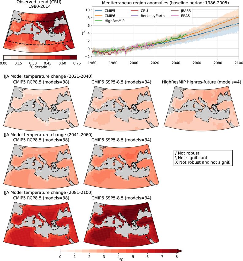
322                          J. Cos et al.: The Mediterranean climate change hotspot in the CMIP5 and CMIP6 projections

and have severe vulnerabilities to climate change and vari-        constraints (Cox et al., 2018; Hall et al., 2019; Tokarska et al.,
ability (Barros et al., 2014). The observed warming in the         2020), performance-based model subsets (McSweeney et al.,
Mediterranean region during the last decades is expected to        2015; Langenbrunner and Neelin, 2017; Herger et al., 2019)
continue and grow larger than the global-mean warming (Li-         and model weighting accounting for performance and inde-
onello and Scarascia, 2018). Additionally, total precipitation     pendence (Knutti et al., 2017; Lorenz et al., 2018; Brunner
declines were observed during the late 20th century (Longo-        et al., 2019). The last approach has been used in this study as
bardi and Villani, 2010), and have been projected by differ-       it additionally considers the interdependencies existing be-
ent multi-model ensembles for the 21st century (Paeth et al.,      tween the models.
2017; Zittis et al., 2019). Characteristics of the projected          This study evaluates and quantifies the Mediterranean cli-
Mediterranean climate change have been linked to thermo-           mate change hotspot for each season over the 21st century
dynamic sources such as land–ocean warming contrast and            by looking into surface air temperature and precipitation
lapse rate change in summer (Brogli et al., 2019), and to dy-      changes in the Mediterranean and how they relate to larger-
namical processes such as the changes in upper-tropospheric        scale responses. We consider three different emission scenar-
large-scale flow in winter (Tuel and Eltahir, 2020).               ios in order to assess the impact of anthropogenic emission
   Numerical models are used to estimate future climate            uncertainties over the Mediterranean climate. The CMIP5
change. Accounting for the physical processes and inter-           and CMIP6 multi-model ensembles are used to estimate the
actions in each climate subsystem (atmosphere, biosphere,          climate change signal, its uncertainty and to illustrate the dif-
cryosphere, hydrosphere and land-surface), global climate          ferences between the two experiments in the region. Finally,
models (GCMs) aim to project the state of the future climate       a weighting method is applied to each CMIP ensemble based
system. Model runs over long historical or future periods are      on the criteria of model performance and independence to
driven by natural forcings (i.e. solar irradiance and volcanic     obtain more robust projections.
aerosols) and anthropogenic emissions that alter greenhouse           Section 2 describes the climate models and observational
gas (GHG) concentrations, leading to changes in the radiative      data used, and explains the methods used to quantify cli-
forcing (Hawkins and Sutton, 2011). GCMs are developed             mate change and weight the projection members. The cli-
by a number of institutions who always apply the same phys-        mate change hotspot in the Mediterranean and the weighted
ical principles but might use slightly different assumptions.      and unweighted projected changes are presented in Sect. 3,
This opens the door to performing the same experiments with        while these results are discussed in Sect. 4. Section 5 con-
multiple GCM outputs, leading to more robust estimates.            cludes and raises questions for further investigation.
Modelling uncertainty can be sampled by ensembling var-
ious models (Tebaldi and Knutti, 2007), while running the
same model multiple times (referred to as members), with           2     Data and methods
differing initial conditions (Eyring et al., 2016), under the
same experiment samples’ internal variability (Hawkins and         2.1    Model data
Sutton, 2011). To make the results comparable, intercom-
parison projects, where several models perform standardized        This study is based on the CMIP5 and CMIP6 historical
experiments, have been organized by the international com-         and future climate projections experiments. The historical
munity (Meinshausen et al., 2011; Riahi et al., 2016). The         CMIP5 experiments span from 1850 to 2005 (Taylor et al.,
main community effort is the Coupled Model Intercompari-           2012) and from 1850 to 2014 in CMIP6 (Eyring et al., 2016).
son Project (CMIP). In this study, we consider the two lat-        The future projections are a continuation of the historical
est CMIP phases, CMIP5 and CMIP6 (Taylor et al., 2012;             simulations, and we have used runs continuing until the year
Eyring et al., 2016), and explore their similarities and differ-   2100. The variables are monthly mean near-surface air tem-
ences over the Mediterranean region. The almost 10 years be-       perature (TAS), precipitation rate (PR) and sea-level pressure
tween CMIP5 and CMIP6 allowed for improvements in the              (PSL). The latter is used to weight the ensemble members to-
modelling of certain Earth system processes such as cloud          gether with TAS (see Sect. 2.3).
feedbacks, aerosol forcings and aerosol–cloud interactions            The increasing computational power over time has al-
(Voosen, 2019; Wang et al., 2021).                                 lowed for increased model resolution and complexity, which
   CMIP experiments were performed with a large set of             leads to the expectation that models have improved from
models and therefore show many differences in projected            CMIP5 to CMIP6. Additionally, we have used the High
changes due to internal variability and the diverse model de-      Resolution Model Intercomparison Project (HighResMIP), a
signs used by the modelling teams. Weighting single model          CMIP6-endorsed MIP (Haarsma et al., 2016) that aims to
runs according to their performance in simulating the ob-          compare lower- and higher-resolution versions of the same
served past allows constraining the climate modelling uncer-       global models. The historical and future HighResMIP pe-
tainty and obtaining a potentially more accurate estimate of       riods span from 1950 to 2014 and from 2015 to 2050 re-
regional climate change signals. Various studies have used         spectively. Though only a subset of the CMIP6 models con-
different subsetting/weighting approaches such as emergent         tributed to HighResMIP, this smaller ensemble has also been

Earth Syst. Dynam., 13, 321–340, 2022                                                  https://doi.org/10.5194/esd-13-321-2022
J. Cos et al.: The Mediterranean climate change hotspot in the CMIP5 and CMIP6 projections                                   323

considered in this study in order to assess the impact of in-      2.3     Methods
creasing model resolution on the Mediterranean climate.
                                                                   All datasets are regridded to a 1◦ × 1◦ grid using a conserva-
   Three radiative forcing scenarios are used to account for
                                                                   tive interpolation method to allow comparison between dif-
uncertainty in future emissions: the CMIP5 Representative
                                                                   ferent models and observational references. After regridding,
Concentration Pathways (RCPs; van Vuuren et al., 2011) 2.6,
                                                                   the dataset’s original orography will differ from that of the
4.5 and 8.5 and the CMIP6 Shared Socioeconomic Path-
                                                                   1◦ × 1◦ grid. Therefore, the TAS values obtained for a spe-
ways (SSPs; Riahi et al., 2016) 1-2.6, 2-4.5 and 5-8.5. The
                                                                   cific altitude might suffer a shift in altitude, which needs to
magnitudes 2.6, 4.5 and 8.5 (in W m−2 ) represent the 2100
                                                                   be corrected by means of the 6.49 K km−1 standard lapse
global radiative forcing in comparison to the pre-industrial
                                                                   rate (Weedon et al., 2011; Dennis, 2014). This is only nec-
era. However, even if the radiative forcing at the end of
                                                                   essary when absolute climatologies are used, as computing
the century is the same in both RCPs and SSPs, the path
                                                                   the change in TAS climatology from one period to the other
to reach it can differ substantially, leading to differences in
                                                                   cancels out this height shift.
the projected climate (Wyser et al., 2020). One of the main
                                                                      To assess the seasonal dependence of climate change
differences between the SSPs and RCPs is that the former
                                                                   over the Mediterranean region, results are computed for the
have a compatible socioeconomic scenario associated with
                                                                   winter months December–January–February (DJF), spring
each forcing scenario, SSP1 being based on sustainability,
                                                                   months March–April–May (MAM), summer months June–
inclusive development and inequality reduction, SSP2 repre-
                                                                   July–August (JJA) and autumn months September–October–
senting a middle-of-the-road scenario, where slow progress
                                                                   November (SON). A summary of the time periods used and
is made in achieving sustainable development goals and
                                                                   the applications of the different diagnostics can be found in
with a mild decline in resource and energy use and being
                                                                   Table 2.
SSP5 based on fossil-fuelled development, rapid technologi-
                                                                      All calculations have been performed using the Earth Sys-
cal progress and economic growth (Riahi et al., 2016; O’Neill
                                                                   tem Model Evaluation Tool (ESMValTool). ESMValTool is
et al., 2016). The results from CMIP5 and CMIP6 sharing the
                                                                   a community framework that facilitates the processing of
same 2100 radiative forcing will be displayed together for
                                                                   generic climate datasets, allowing for reproducibility of re-
simplicity, but the reader should always bear in mind that the
                                                                   sults (Righi et al., 2020).
evolution of GHG concentrations differs between them. They
                                                                      Mediterranean TAS and PR are assessed over land to high-
are not entirely comparable as RCPs and SSPs defined with
                                                                   light the impact of climate change over populated regions.
the same radiative forcing at the end of the century do not
                                                                   This avoids values over sea influencing results over land
share the same progression of aerosol and GHG concentra-
                                                                   when regridding is performed, i.e. TAS behaves differently
tions throughout the 21st century. HighResMIP is only avail-
                                                                   over land than over sea due to differences in surface thermo-
able for the scenario SSP5-8.5 for future projections.
                                                                   dynamic properties, while PR over sea should not have an
   Many of the models have more than one member, meaning
                                                                   impact on freshwater resources over land.
that the model runs have been started with different initial
conditions, leading to diverging climate trajectories. The aim
of having multiple members is to sample the uncertainty that       2.3.1    Projections verification
arises from internal variability (Lehner et al., 2020; Deser       To verify the projection ensembles used, we compare the lin-
et al., 2020). Having multi-member models means that the           ear trend (TREND) distributions of the observational prod-
multi-model ensembles are super-ensembles. A summary of            ucts against the multi-model ensembles. This is computed by
the simulations performed by each model used and for every         applying the linear ordinary least square regression fit with
scenario can be found in Appendix A.                               time as an independent variable. The 35-year period 1980–
                                                                   2014 has been used to calculate trends in each model and
2.2   Observational data                                           observational dataset, as a period with shorter span would be
                                                                   too dependent on the effect of internal variability from the
We use observational references to compare the model ex-
                                                                   climate system (Merrifield et al., 2020; Peña-Angulo et al.,
periments to the observed past and to derive performance
                                                                   2020). Note that CMIP5 years 2006–2014 are taken from the
weights of ensemble members. Multiple observational prod-
                                                                   corresponding scenario simulation. The results are gathered
ucts are used including both reanalysis (ERA5 and JRA55)
                                                                   in the respective OBS, CMIP5, CMIP6 and HighResMIP dis-
and gridded observations (GPCC, CRU, BerkeleyEarth and
                                                                   tributions (displayed as box plots), and we perform a quali-
HadSLP2) to account for observational uncertainty. A sum-
                                                                   tative assessment on the differences between observed and
mary of the observational datasets used is found in Table 1.
                                                                   simulated historical trends.
JRA55 will not be displayed in the time series plots as it over-
estimates the precipitation over the Mediterranean during the
period 1958–1978 (Tsujino et al., 2018).                           2.3.2    Mediterranean hotspot evaluation
                                                                   A climate change hotspot is defined as a region whose
                                                                   climate is especially responsive to global change (Giorgi,

https://doi.org/10.5194/esd-13-321-2022                                                Earth Syst. Dynam., 13, 321–340, 2022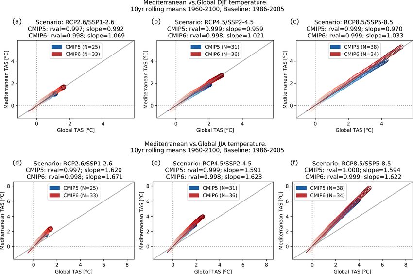
324                              J. Cos et al.: The Mediterranean climate change hotspot in the CMIP5 and CMIP6 projections

Table 1. Summary of the observational references for near-surface air temperature (TAS), precipitation rate (PR) and sea-level pressure
(PSL).

         Name             Type                   Institute                               Variables        Reference
         JRA55            Reanalysis             Japan Meteorological Agency (JMA)       TAS, PR, PSL     Kobayashi et al. (2015)
         ERA5             Reanalysis             European Centre for Medium-Range        TAS, PSL         Hersbach et al. (2020)
                                                 Weather Forecasts (ECMWF)
         CRU (v4.04)      Gridded observations   University of East Anglia (UEA)         TAS, PR          Harris et al. (2020)
         GPCC (v2018)     Gridded observations   Deutscher Wetterdienst (DWD)            PR               Schamm et al. (2014)
         BerkeleyEarth    Gridded observations   Berkeley Earth                          TAS              Rohde et al. (2013)
         HadSLP2          Gridded observations   Met Office (UKMO)                       PSL              Allan and Ansell (2006)

Table 2. Summary of each diagnostic’s use and time period.

             Diagnostic   Period(s)                                                Use
             1            2021–2040/2061–2080/2081–2100 against 1986–2005          weighted and unweighted projection results
             DIFF         1980–2014                                                performance weight
             STD          1980–2014                                                performance weight
             TREND        1980–2014                                                performance weight and verification
             CLIM         1980–2014                                                independence weighting

2006). To characterize the hotspot, we compare the TAS                guidelines from IPCC (2021). Additionally, as CMIP5 his-
and PR behaviours in the Mediterranean against the global             torical simulations end in 2005, the reference period 1986–
and latitudinal band responses respectively. The first step           2005 from IPCC’s AR5 (Collins et al., 2013) is chosen to
is to calculate the change in the variables’ magnitude be-            avoid overlapping historical and scenario experiments when
tween the reference period (1986–2005, from Collins et al.,           extracting projection results. Note that only the near-term pe-
2013) climatology (CLIM) and a future period CLIM (this               riod is available for HighResMIP as the future experiment
diagnostic is referred to as 1 in this text). To evaluate the         ends in 2050. The advantage of using 1 instead of future
TAS hotspot, we compute the differences between the multi-            CLIMs is that the GCMs’ mean-state systematic biases are
model Mediterranean land-only 1TAS and the global land–               removed, and we obtain a more easily interpretable compari-
ocean 1TAS means (Lionello and Scarascia, 2018). For PR               son of the responses among models and between models and
the land–ocean latitudinal belt 30–45◦ N mean is used in-             observations (Garfinkel et al., 2020).
stead of the global mean (Lionello and Scarascia, 2018). To              With the aim to sample the inherent uncertainty of the
highlight the difference in the impact of the hotspot within          multi-model ensemble, we compute the inter-model spread
the Mediterranean region, we plot the hotspot maps using              from the 5th and 95th percentiles of the ensemble distribu-
the near-term and long-term 1, which refer to the future pe-          tion. To take into account the scenario uncertainty, we dis-
riods 2041–2060 and 2081–2100 respectively. Additionally,             play the distribution of 1 from the three different scenarios
to assess the evolution of the hotspot, we calculate the pro-         that we have used for each ensemble side by side (RCP2.6,
jected area-averaged 10-year rolling windows of the Mediter-          RCP4.5 and RCP8.5 for CMIP5 and SSP1-2.6, SSP2-4.5 and
ranean 1 and the large-scale 1 for both TAS and PR. For               SSP5-8.5 for CMIP6).
precipitation, the area aggregations are computed using ab-              The statistical significance of TAS and PR mean changes
solute values and then the relative change with respect to the        and the degree of agreement between the models are used
reference is calculated (displayed in percentage).                    to assess the uncertainty and robustness of the multi-model
                                                                      ensemble results. A climate change signal is considered ro-
2.3.3     Mediterranean projected changes quantification              bust when at least 80 % of the models agree on the projected
                                                                      sign of the 1s (Collins et al., 2013). A change in the multi-
To quantify the projected magnitudes of Mediterranean re-             model mean is considered significant when it is beyond the
gion climate change, we compute 1 between the reference               threshold of a two-tailed paired t test (Ukkola et al., 2020)
period 1985–2005 and the future periods: near term (2021–             at the 95 % confidence level. The paired t test is chosen be-
2040), mid-term (2041–2060) and long term (2081–2100).                cause it is invariant to differences in the sample’s variability.
We use 20-year baseline and future periods following the

Earth Syst. Dynam., 13, 321–340, 2022                                                      https://doi.org/10.5194/esd-13-321-2022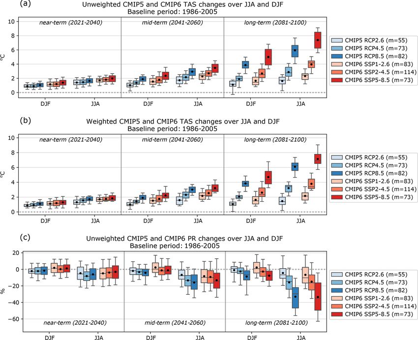
J. Cos et al.: The Mediterranean climate change hotspot in the CMIP5 and CMIP6 projections                                    325

We consider that the null hypothesis is met when there is no         diagnostics are the surface temperature 1980–2014 CLIM
difference between the multi-model distribution in the refer-        minus its area average (TAS-DIFF), the surface temperature
ence and future periods. To compute the t statistic, first, each     interannual standard deviation (TAS-STD), the surface tem-
model’s mean is computed from its members, and secondly,             perature linear trend (TAS-TREND), the sea-level pressure
the multi-model ensemble mean and standard deviation are             1980–2014 CLIM minus its area-average (PSL-DIFF) and
calculated.                                                          the sea-level pressure interannual standard deviation (PSL-
                                                                     STD). The independence diagnostics are the 1980–2014 PSL
2.3.4   Weighting method                                             and TAS climatologies (PSL-CLIM and TAS-CLIM).
                                                                        The distances between member-observations for each
It has been argued that more robust projections could be ob-         of the diagnostics are aggregated as in Eq. (2) where
tained by giving more weight to members with good perfor-            di represents the distance for each diagnostic X d =
mance (Knutti et al., 2017). Therefore, we compare histori-          (TAS-TREND, TAS-DIFF, TAS-STD, PSL-DIFF, PSL-STD).
cal simulations against the observational ensemble mean and          Equation (3) shows how to compute the distances between
more weight is given to those members that better reproduce          models and observations, where g refers to each grid cell and
the observed climate, i.e. weighting them by performance.            wg represents its area weight. To find Sij the same method
Another aspect that can be taken into account when weight-           is followed but using Xs = (TAS-CLIM, PSL-CLIM)
ing a multi-model ensemble is the independence between               and comparing members against each other instead of
members. Giving equal weight to all members (one model               observations.
one vote) is not a fair approach as some share model formu-                                     d
lations (either because their runs belong to the same model                   X           diX
                                                                     Di =                                                      (2)
or because their models share similarities), and would be

                                                                                                 d
                                                                               Xd    MEDIANi diX
overrepresented in the ensemble. An independence weight-                         s
ing method is applied to correct this issue.                             d           X
                                                                                                d 2
                                                                     diX              wg Xid − Xobs

                                                                             =                                                 (3)
   Using the approach developed in Lorenz et al. (2018),
                                                                                     g
Brunner et al. (2020) and Merrifield et al. (2020), we use
Eq. (1) to give a weight wi to each member i in the pro-                The shape parameters are constant values that determine if
jections ensemble. The distances (measured with the root             the member-observations or the member–member distances
mean squared error, RMSE) Di between member i and the                are enough to downweight a member (σd ) or if they are close
observational reference inform the performance weight, and           enough to determine some dependency between members
the distance Sij between member i and every other mem-               (σs ) respectively. Each ensemble (CMIP5 and CMIP6), sea-
ber j from the multi-model ensemble informs the indepen-             son and scenario has its own associated shape parameters.
dence weight. The amount of j members is represented by m,           Appendix B explains in further detail the meaning of the
which is the total number of members minus one. σs and               shape parameters, the methods used to compute them and
σd are the independence and performance shape parameters             the diagnostics used to determine performance and indepen-
respectively. The mean of the observational ensemble is used         dence.
as the observational reference.
                              2
                                                                     3       Results

                         Di
                 −       σd
             e
wi =                                                          (1)
             Pm               −
                                   S 2
                                    ij                               Apart from the figures displayed in this section and the
                                   σs
        1+       j 6 =i e                                            Supplement, additional ones generated during the study
                                                                     can be found in a shiny app in the following link https:
    The weighting method distances account for different per-        //earth.bsc.es/shiny/medprojections-shiny_app/ (last access:
formance and independence diagnostics (trends, differences,          December 2021).
variabilities and climatologies) to avoid weighting members
that could match the performance and independence criteria
                                                                     3.1      Verification
of a single diagnostic just by chance. The diagnostics di and
sij , respectively used to evaluate the distances Di and Sij , are   We compare CMIP and HighResMIP ensemble TAS and PR
different, as Merrifield et al. (2020) suggests. The aim when        trends to the observational ensemble trends between 1980
evaluating performance is to give more weight to members             and 2014 as an indication of model performance over the
that resemble the observed past in a more faithful way. Dif-         Mediterranean. PR and TAS trends in the observational en-
ferently, the aim of weighting for independence is to clearly        semble fall within the range of the multi-model ensem-
identify members that behave in a similar way. All the di-           bles in all seasons (see Fig. 1 for DJF and JJA results;
agnostics are computed over the period 1980–2014 (Brunner            MAM and SON not shown). The historical multi-model en-
et al., 2020). The variables used to compute the diagnostics         semble spread of temperature trends is notably larger than
are TAS and PSL (Merrifield et al., 2020). The performance           that of the observational ensemble. CMIP6 past warming

https://doi.org/10.5194/esd-13-321-2022                                                      Earth Syst. Dynam., 13, 321–340, 2022
326 J. Cos et al.: The Mediterranean climate change hotspot in the CMIP5 and CMIP6 projections
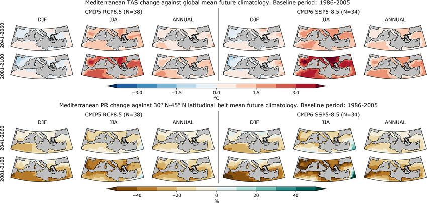
3.2 The Mediterranean as a climate change hotspot
Figure 2 shows CMIP5 and CMIP6 high radiative forcing
scenario differences of 1TAS over the Mediterranean against
the 1986–2005 global-mean 1TAS (for DJF, JJA and the an-
nual means). The Mediterranean 1PR is compared to the 30–
45◦ N latitudinal belt 1PR mean.
The Mediterranean region shows a higher annual tempera-
ture increase than the global mean. When accounting for sea-
sonal differences, the highest amplifications are visible for
JJA over the Iberian Peninsula and the Balkans. CMIP5 and
CMIP6 agree on the regions showing the highest amplified
warming, but the latter projects larger amplification magni-
tudes. There is agreement between both CMIPs in the dis-
tribution and magnitude of the DJF warming amplification,
which is small and even negative in the north-west part of the
domain. While projections agree on a precipitation increase
in the 30–45◦ N latitudinal belt for the long-term period (Li-
onello and Scarascia, 2018), the Mediterranean region shows
a decline in precipitation. The largest amplified drying shifts
latitudinally from the south of the Mediterranean region in
DJF to the north in JJA. The most affected region in JJA
Figure 1. Historical trends for DJF (a, b) and JJA (c, d) temper- is projected to be the south-west of the Iberian Peninsula.
ature (a, c) and precipitation (b, d) of the observational, CMIP5, Both CMIPs agree on the precipitation patterns of change,
CMIP6 and HighResMIP ensembles. The observational distribution but CMIP6 dries more and faster in the amplified drying re-
is composed of the different values obtained from each of the ob- gions, and projects larger precipitation increases in regions
servational products. In the box plots, the black horizontal line rep- where the hotspot has a negative sign such as the south-east
resents the median and the black dot is the mean. The interquartilic of the domain (probably enhanced by using relative precipi-
range (IQR) and whiskers are defined by the 25th–75th and 5th– tation changes).
95th percentiles respectively. HighResMIP models are displayed as TAS and PR differences increase in magnitude from the
markers, enabling a comparison of the HR (green) and LR (orange)
mid- to the long term, while the spatial pattern remains
models within the experiment. The same markers are used for two
different resolution runs of the same model (see Table S1 in the
the same, indicating that the climate in the Mediterranean
Supplement). changes faster than the global average when forced by the
8.5 W m−2 scenarios. The low emission scenario, instead,
shows a hotspot weakening from the mid- to the long term
trends are generally larger than CMIP5. The inter-model as the warming amplification is reduced and the precipitation
spread for the precipitation projections is large for all en- differences are maintained (see Fig. S1 in the Supplement).
sembles and usually has both negative and positive trends The weakening of the hotspot under the low emission sce-
(e.g. DJF CMIP5 precipitation trends range from −0.092 to nario will be further explored below.
0.097 mm d−1 decade−1 for the 5th and 95th percentiles re- Even though CMIP6 projects a larger warming and dry-
spectively). HighResMIP TAS trends are contained within ing amplification than CMIP5, Fig. 3 shows that CMIP5 and
the CMIP6 ensemble, but some of the high-resolution (HR) CMIP6 agree on the relation between global and local warm-
models exhibit trends outside the CMIP6 range for PR in ing (slopes drawn in the figures). This indicates that CMIP6
JJA (Fig. 1d). The agreement between the different obser- does not enhance the hotspot with respect to CMIP5, but
vational products in past warming trends is shown in Fig. S7 rather the higher amplified warming in the Mediterranean is
(columns 1 and 5). While the general warming patterns are the result of a globally warmer multi-model ensemble. For
similar, there are some notable differences over the Balkans DJF, additional warming over the Mediterranean is almost
and western Asia. The figure also highlights the need to con- zero with respect to the global mean. Contrastingly for JJA,
sider multiple observational sources, as historical trends dif- additional warming over the Mediterranean is about 1.6 times
fer both in magnitudes and spatial patterns. higher than the global-mean warming. This relationship ap-
pears to be linearly maintained for higher global warming
levels, i.e. with time and GHG concentrations.
In spite of this strong agreement in the relationship be-
tween global and local warming, CMIP5 and CMIP6 have
slight differences in the projected precipitation over the
Earth Syst. Dynam., 13, 321–340, 2022 https://doi.org/10.5194/esd-13-321-2022J. Cos et al.: The Mediterranean climate change hotspot in the CMIP5 and CMIP6 projections 327 Figure 2. Mediterranean region TAS (upper rows) and PR (lower rows) change differences with respect to the mean global temperature change and the mean 30–45◦ N latitudinal belt precipitation change respectively. The changes for the periods 2041–2060 (first and third row) and 2081–2100 (second and fourth row) are evaluated against the 1986–2005 mean. The differences are shown for the CMIP5 (left) and CMIP6 (right) DJF, JJA and annual mean projections (columns) under the high emission scenario RCP8.5 and SSP5-8.5 respectively. N indicates the number of models included in the ensemble mean. Figure 3. Mediterranean region warming against global warming for the three scenarios (columns) shown in DJF (a–c) and JJA (d–f) for the CMIP5 and CMIP6 ensemble means. Each dot represents a 10 year mean change beginning from 1960–1969 (light colouring) until 2091– 2100 (opaque colouring). The changes are computed with 1986–2005 as baseline. An ordinary least squares linear regression is computed and the slope and r values are shown. N indicates the number of models included in the ensemble mean. https://doi.org/10.5194/esd-13-321-2022 Earth Syst. Dynam., 13, 321–340, 2022
328 J. Cos et al.: The Mediterranean climate change hotspot in the CMIP5 and CMIP6 projections
Mediterranean in comparison to the 30–45◦ N latitudinal belt HR and low-resolution (LR) projections are contained within
(see Fig. S2). CMIP5 generally shows more negative slopes the CMIP5 and CMIP6 distributions (only near term; see
than CMIP6, meaning that the former is projecting a larger Fig. S5c). No specific relation between the LR and HR model
amplification of the precipitation hotspot as the relative pre- outputs can be found, and due to the small size of the High-
cipitation loss in the Mediterranean (ordinate) for the same ResMIP ensemble, further conclusions cannot be drawn. Fi-
amount of precipitation increase in the larger-scale region nally, from the area-averaged distributions of 1TAS (Fig. 4a)
(abscissa) is larger. While this is true for all seasons and sce- we can see that the largest source of uncertainty for the mid-
narios, the difference between CMIP5 and CMIP6 is more and long term is the forcing scenario, and the inter-model
noticeable during DJF and especially for the low emission spread for the near term.
scenario. Figure S3 highlights more extreme relative CMIP6 The inter-model spread grows larger with emissions both
precipitation changes in the latitudinal band and increases of for TAS and PR (Fig. 4a and c). To check the influence of the
over 30 % in Asia and over the Pacific as opposed to CMIP5. equilibrium climate sensitivity (ECS) on the increasing inter-
Therefore, conclusions must be drawn carefully from com- model spread, the same plot is computed with a subset of
paring area-averaged values of these regions. Nevertheless, CMIP5 and CMIP6 models with ECSs constrained between
there is agreement between both ensembles on the spatial 2.6 and 3.3 ◦ C (rather than the original 2.1 to 4.7 ◦ C ECS
distribution of PR changes. range from CMIP5, Meehl et al., 2020 and the 1.8 to 5.6 ◦ C
We tried following a second approach to assess the trend ECS range from CMIP6, Hausfather, 2019). From Fig. S6 it
differences of the precipitation hotspot between the CMIPs. can be seen that ensembles with narrower ECS ranges show
Figure S4 shows changes in precipitation for the Mediter- a reduction in inter-model spread growth over time for the
ranean region against the global-mean warming, and the en- high emission scenarios.
semble that dries faster for the same magnitude of global Figure 5 shows the spatial distribution of the projected JJA
warming is CMIP5. This is more noticeable during the DJF warming in the high emission scenario for CMIP5, CMIP6
season. The results from Fig. S4, together with Fig. S2, give and HighResMIP in the three future reference periods. JJA
evidence supporting that CMIP5 projects a larger precipita- warming is significant and robust for the three future peri-
tion hotspot (relative to its own large-scale climate response) ods in the Mediterranean region (see Fig. 5). As seen before,
than CMIP6. CMIP6 warms more than CMIP5 and at a faster rate. Never-
Coming back to the hotspot weakening, the low emission theless, there is good spatial agreement between the warming
scenario panels (Figs. S2a and d and S4a and d) show more projected by the CMIP experiments over the Mediterranean
clearly how a recovery of the precipitation decline is pro- region. The Iberian Peninsula, the Balkans and Eastern Eu-
jected following mitigation. For the rest of the scenarios, rope are the regions with the largest mean JJA warming, with
the projected amplified warming, combined with an anoma- values reaching over 8 ◦ C.
lous precipitation decline, makes the Mediterranean a climate The remaining scenarios also project robust and signifi-
change hotspot (Lionello and Scarascia, 2018). cant warming for JJA throughout the century with a tendency
of smaller positive trends by 2050 (not shown). CMIP6 sys-
tematically projects higher warming than CMIP5 again with
3.3 Unweighted projections a similar spatial warming pattern. The regions with larger
3.3.1 Temperature warming are the Iberian Peninsula and the Balkans.
The temperature spatial changes during DJF for the high
Figure 4a shows projected multi-model ensemble JJA and emission scenario are shown in Fig. S8. The north-eastern
DJF TAS changes under three scenarios and three time hori- Mediterranean shows the largest projected warming in DJF
zons over the Mediterranean. The CMIP6 ensemble always (4.5 ◦ C according to CMIP5 and 6 ◦ C to CMIP6). For the
shows larger 1TAS than CMIP5. The inter-model spread near term, HighResMIP shows a slightly larger TAS increase
for the end of the century is larger for CMIP6 than CMIP5. than CMIP6 in eastern Europe. The rest of scenarios agree
CMIP6 projects JJA temperatures to increase by over 7.4 ◦ C with the spatial distribution of changes but with lower warm-
(90 % inter-model spread within 5.6 to 9.1 ◦ C) by the end ing magnitudes (not shown).
of the century under the high emission scenario and 2.3 ◦ C
(90 % within 1.2 to 3.3 ◦ C) under the low emission scenario 3.3.2 Precipitation
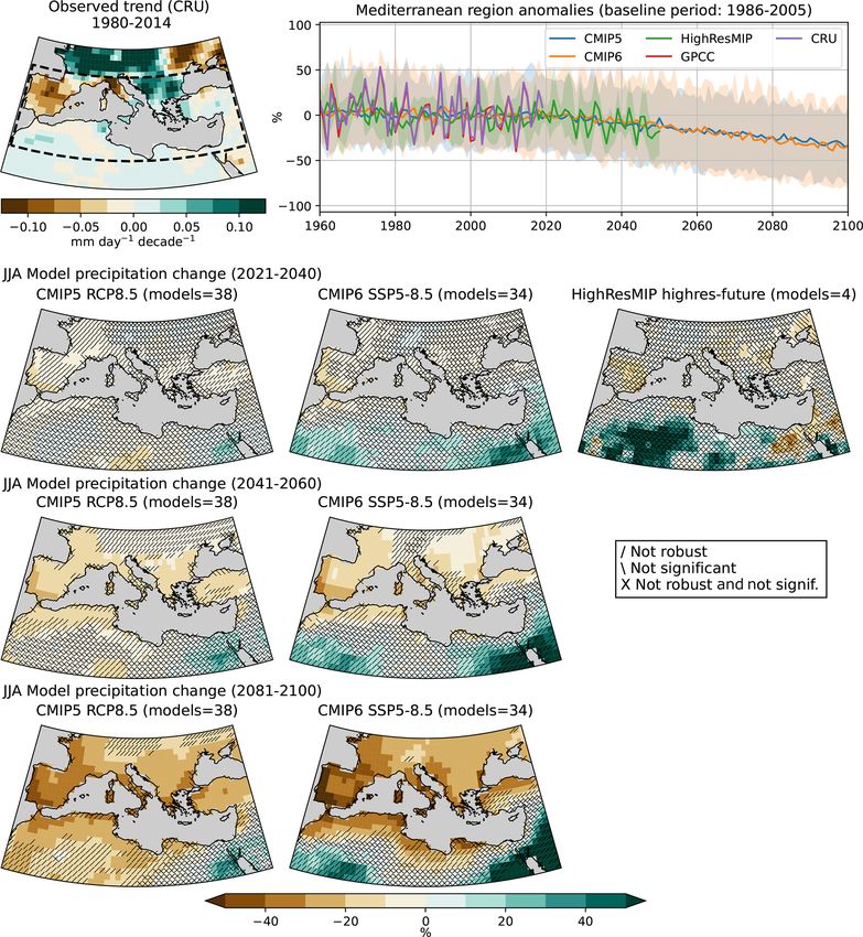
(Fig. 4). CMIP5 shows a mean JJA warming of 5.9 ◦ C by the
end of the century (90 % within 4.1 to 7.7 ◦ C) under RCP8.5 In contrast to temperature, CMIP5 and CMIP6 show the
and 1.6 ◦ C (90 % within 0.3 to 2.5 ◦ C) under RCP2.6. In DJF same mean JJA 1PR declines of −33 % by the end of the
the warming is always lower, and 90 % of CMIP6 models century under the high emission scenario (Fig. 4c). CMIP6
for the high emission scenario project a 1TAS within 3.3 has a wider inter-model 90 % range than CMIP5. The former
to 6.8 ◦ C (CMIP5: 2.7 to 5.0 ◦ C). For the remaining seasons spans −63 % to −4 % and the latter −56 % to −11 %. For
(MAM and SON), CMIP6 shows a larger warming and larger the low emission scenario CMIP6 mean JJA precipitation de-
intermodel spread than CMIP5 (not shown). HighResMIP clines by −7 % (90 % within −23 % to +17 %) and CMIP5
Earth Syst. Dynam., 13, 321–340, 2022 https://doi.org/10.5194/esd-13-321-2022J. Cos et al.: The Mediterranean climate change hotspot in the CMIP5 and CMIP6 projections 329
Figure 4. CMIP5 and CMIP6 JJA and DJF projections for the near-, mid- and long-term periods with respect to the baseline period consider-
ing the 2.6, 4.5 and 8.5 W m−2 RCP and SSP radiative forcing scenarios for (a) unweighted 1TAS, (b) weighted 1TAS and (c) unweighted
1PR. The black horizontal line in the boxes represents the median and the black dot is the mean. The interquartile range (IQR) and whiskers
are defined by the 25th–75th and 5th–95th percentiles respectively. The number of members in the boxplot distributions is represented by m
in the legend.
by −4 % (90 % within −19 % to +16 %). In DJF and by the for long-term JJA projections, and the inter-model spread for
end of the century, CMIP6 precipitation declines by −8 % DJF and near and mid-term JJA.
(90 % within −20 % to +5 %) and CMIP5 by −9 % (90 % Precipitation spatial changes in the Mediterranean region
within −31 % to +4 %) under the high emission scenario. only become more robust and significant with time (see
For the low emission scenario in DJF, CMIP6 shows a mean Fig. 6). 1PR projected for the long term during JJA, and un-
+2 % precipitation increase (90 % within −11 % to +18 %) der the 8.5 W m−2 scenarios, indicate significant and robust
and CMIP5 a −1 % decline (90 % within −15 % to 9 %). decline for most of the region. The mid-term 8.5 W m−2 and
Seasons JJA, DJF (Fig. 4c), MAM and SON (not shown) for the long-term 4.5 W m−2 scenarios show locally robust and
all scenarios generally project mean 1PR declines beginning significant changes in the Iberian Peninsula and north of the
from the mid-term period onwards. Nevertheless, there is an Pyrenees. Both CMIPs agree on the south-western Iberian
exception in DJF under the low emission scenario, where a Peninsula having the strongest precipitation decline, with
slight increase in mean DJF precipitation is projected. High- long-term CMIP6 changes ranging from −50 % to −60 %
ResMIP near-term projections of PR change are contained and CMIP5 from −30 % to −40 % for the high emission sce-
within the CMIP6 ensemble (Fig. S5b and d). Generally, the nario. Despite lower forcing scenarios projecting less robust
signal is considerable, but the inter-model spread is wide for and significant changes (except the western Mediterranean
all multi-model ensembles; therefore, we will later present for long-term SSP2-4.5), the results agree on a general pre-
the statistical robustness and significance of changes. Finally, cipitation decline throughout the region with patterns similar
from the area-averaged distributions of 1PR (Fig. 4c), we see to high emission scenario projections (not shown). The High-
that the largest source of uncertainty is the forcing scenario ResMIP projections agree with CMIP6 mean magnitudes and
spatial pattern for most of the seasons in the near-term pe-
https://doi.org/10.5194/esd-13-321-2022 Earth Syst. Dynam., 13, 321–340, 2022330 J. Cos et al.: The Mediterranean climate change hotspot in the CMIP5 and CMIP6 projections Figure 5. JJA 1TAS according to CMIP5, CMIP6 and HighResMIP ensemble means (columns) for the three relevant future periods (rows), under the RCP8.5 and SSP5-8.5 scenarios. The time series plot shows the anomalies in the Mediterranean region with respect to the period 1986–2005 for the multi-model ensembles and the observational references. A solid line indicates the one-member-per-model ensemble mean and the shaded region indicates the 5th–95th percentiles range. The CRU trend for the period 1980–2014 is shown along with the dashed line, which bounds the Mediterranean region. riod (the large amount of non-robust and non-significant grid 3.4 Weighted projections points must be noted). 1PRs in DJF are different from those in JJA (see Fig. S9). The models of CMIP ensembles perform very differently de- The southern part of the domain is expected to see a signif- pending on the computed diagnostic, and some models share icant and robust precipitation decline in the long term of up similarities. Section 1 of the Supplement explains in further to −20 % to −40 % over northern Africa. The north of the detail how differently models represent the observed climate Mediterranean is located in a transition zone, as precipitation over the Mediterranean region, justifying the need to con- in areas north of the Pyrenees, Alps and Balkan Peninsula is strain the projection ensembles. projected to increase and in areas under 38◦ N is projected to We obtain new projections from applying the performance decrease, causing changes for the Iberian, Italian and Balkan and independence weighting method to TAS projections peninsulas to remain uncertain. In comparison to CMIP5, from the CMIP5 and CMIP6 ensembles. Figure 4b shows CMIP6 shows a wider 5th–95th percentile spread over the the distribution of 1TAS in the weighted ensembles for the Mediterranean region for all the scenarios considered (2.6 three emission scenarios and the three future periods. The and 4.5 W m−2 scenarios are not shown). As a final remark, weighting increases the CMIP5 mean and median projec- the observed DJF precipitation variability in the time series tions while at the same time decreasing the CMIP6 mean falls outside the simulated 90 % inter-model spread (5th-95th and median projections, bringing the two ensemble means percentiles shown in shading in Fig. 6). closer together: before weighting, the CMIP5 and CMIP6 Earth Syst. Dynam., 13, 321–340, 2022 https://doi.org/10.5194/esd-13-321-2022
J. Cos et al.: The Mediterranean climate change hotspot in the CMIP5 and CMIP6 projections                                      331

Figure 6. Same as Fig. 5 for JJA precipitation and showing CRU in the top left panel.

medians differed by 1.32 ◦ C and after weighting the differ-           both mean distributions smaller. In some cases the weight-
ence is 0.68 ◦ C (for the highest emission scenario in JJA).           ing did not lead to large alterations of the projected inter-
Generally, the high emission scenario means are those that             model spread, suggesting that uncertainties in the tempera-
see larger reductions in the CMIP6 ensemble; e.g. differences          ture changes are well sampled by the original ensembles. In
between the unweighted and weighted ensemble means are                 contrast, the large IQR of CMIP6 model projections in the
around −0.3, −0.2 and −0.1 ◦ C in JJA and DJF for SSPs                 long term is reduced by half, and the CMIP5 90 % inter-
5-8.5, 2-4.5 and 1-2.6 respectively. The IQRs are generally            model spread narrows by up to 1 ◦ C, after weighting. Nev-
narrowed for all seasons and scenarios except for the mid-             ertheless, even though the weighting approach reduces the
and long-term JJA SSP2-4.5, SSP1-2.6 and RCP2.6 scenar-                probability of the most extreme warming values, they remain
ios. The 90 % spreads are slightly reduced or maintained; ex-          possible in the weighted ensemble. Generally speaking, the
ceptions are the CMIP6 DJF long-term distributions and the             90 % inter-model spreads are maintained while the IQRs nar-
CMIP6 JJA low and middle emission scenarios for the mid-               row.
term. The 75th–95th percentile range in the weighted CMIP6                To assess the contribution of the performance and indepen-
ensemble increases while the 5th–25th percentile range de-             dence weights in the resulting distribution, we have plotted
creases, generating a skewed weighted CMIP6 distribution               the distribution of performance and full weights, and com-
towards smaller warming. Weighting the CMIP5 ensemble                  pared the raw ensemble long-term warming distribution with
leads to a more constrained distribution.                              the performance-weighted and the fully weighted warmings
   The weighted 1TAS projections in DJF show similar re-               (Fig. S12). JJA performance shifts both CMIP ensembles to
sponses as in JJA: the mean signal in CMIP6 decreases                  larger warmings, while the addition of independence weights
while it increases in CMIP5, making the differences between            shifts the CMIP6 median to lower warmings than the raw en-

https://doi.org/10.5194/esd-13-321-2022                                                  Earth Syst. Dynam., 13, 321–340, 2022
332                          J. Cos et al.: The Mediterranean climate change hotspot in the CMIP5 and CMIP6 projections

semble. DJF performance weights do not have an effect on           TAS and PR output from the older (CMIP5) and newer gener-
the warming medians but they the narrow CMIP5 spread. The          ation (CMIP6) multi-model ensembles is an enhancement of
addition of DJF independence weighting shifts the CMIP6            the global change, while its relation with the Mediterranean
median warming and broadens its inter-model spread. The            region response has been maintained. The work of Palmer
CMIP5 median remains unchanged but its spread grows to-            et al. (2021) arrives at a similar conclusion for the European
ward the raw distribution without reaching it.                     region.
   Note that precipitation-weighted projections are not shown         The drivers of the projected Mediterranean climate change
as there is no evidence that the diagnostics used to assess        has been studied by Brogli et al. (2018), Brogli et al. (2019)
temperature (Merrifield et al., 2020) are relevant to the pre-     and Tuel and Eltahir (2020). They have found that the mecha-
cipitation response of the models.                                 nisms projected to drive the Mediterranean climate are large-
                                                                   scale upper-tropospheric flow changes (PR in DJF), reduc-
                                                                   tion in the regional land–sea temperature gradient (PR in
4   Discussion                                                     DJF and JJA) and changes in the north–south lapse rate con-
                                                                   trast (PR in JJA, TAS in DJF and JJA). While these drivers
Projections obtained from climate multi-model ensembles            have been deeply studied for CMIP5, affirming that the same
contain various sources of uncertainties. Different modelling      mechanisms remain valid for the CMIP6 ensemble would be
methods and emission scenarios (e.g. land use, GHG emis-           speculative.
sions) lead to different results (Tebaldi and Knutti, 2007). We       Consistent with basic radiative forcing theory (Wallace
use different multi-model ensembles and radiative forcing          and Hobbs, 2006), temperature projections have shown that
scenarios to consider as many factors as possible contribut-       the warming over the 21st century is larger when stronger
ing to the uncertainty of the Mediterranean climate change         radiative forcing scenarios are applied. There is confidence
projections. Additionally, a weighting method constraining         in a precipitation decline for the high emission scenario over
the projections has been applied to reduce uncertainty in the      the whole Mediterranean region in JJA and only in the south
projections.                                                       during DJF. Conclusions should be drawn carefully from pre-
   We have shown that average Mediterranean temperature            cipitation as there is a large inter-model spread. For other
changes were larger than the global-mean average during            seasons and scenarios, precipitation declines are projected,
JJA, but close to it during DJF, for all scenarios, time periods   although results are uncertain due to the large spread and low
and model ensembles. This hotspot is projected to enhance          significance and robustness over most of the region. Regard-
over the 21st century under the scenarios RCP8.5, SSP5-            ing HighResMIP, the HR near-term precipitation and tem-
8.5, RCP4.5 and SSP2-4.5, and to diminish from the mid-            perature changes generally fall within the CMIP6 ensemble
to long term under the RCP2.6 or SSP1-2.6 scenarios. In-           distribution and no clear improvement could be seen from
terestingly, the multi-model ensemble mean projections of          the increased resolution in the historical trends, probably due
the low emission scenario show a recovery of the precipita-        to the small number of HighResMIP models available for the
tion decline towards the end of the century, suggesting that       assessment, and the focus on larger-scale changes and tem-
precipitation could be restored to historical values relatively    poral resolutions.
fast in the Mediterranean region if strict mitigation policies        The largest source of uncertainty in determining the warm-
are applied. Previous studies also have identified the Mediter-    ing and precipitation changes over the mid- and long-term
ranean warming amplification (Lionello and Scarascia, 2018;        periods is the emission scenario (as seen in Fig. 4). To il-
Zittis et al., 2019), but it must be stressed that this enhanced   lustrate scenario uncertainty, let us take the range between
warming does not apply to the DJF season.                          the 5th and 95th percentile of the low (high) and high (low)
   We argue that the different results obtained from CMIP5         emission scenario distributions for temperature (precipita-
and CMIP6 for the Mediterranean hotspot and the un-                tion) changes. CMIP6 shows a range from 1 to 9 ◦ C warm-
weighted projections are largely due to the global response        ing and −62 % to 19 % precipitation long-term changes in
from each multi-model ensemble. Figures 3, S2 and S4 show          JJA. CMIP5 ranges from 0.1 to 7.5 ◦ C warming and −54 %
how the regional changes relative to the larger scale are sim-     to 18 %. This broad spectrum of possible futures has various
ilar for both CMIPs, indicating that CMIP6 is not producing        possible associated outcomes. The inter-model spread grows
a regional enhancement of climate change, but it rather fol-       at faster rates throughout the 21st century with higher radia-
lows a larger global change. This behaviour is most evident        tive forcing, in part due to the differing climate sensitivities
in JJA than in DJF, as the relative changes with respect to        of the models inside the ensemble (see Fig. S6); i.e. the dif-
larger scales are more similar for the two multi-model en-         ferences between a low and a high climate sensitivity model
sembles. To further support this statement, we look at the         will become amplified with larger radiative forcing.
spatial distribution of changes within the Mediterranean re-          The implications of an 8.5 W m−2 increase in radiative
gion in Figs. 5, 6, S3, S8 and S9. The figures generally agree     forcing from preindustrial times by the end of the cen-
on the spatial distribution of changes even if the magnitudes      tury could pose severe strains on human health, due to
differ. Therefore, we can argue that the main difference in        heat-related illnesses (Lugo-Amador et al., 2004) and al-

Earth Syst. Dynam., 13, 321–340, 2022                                                 https://doi.org/10.5194/esd-13-321-2022
J. Cos et al.: The Mediterranean climate change hotspot in the CMIP5 and CMIP6 projections 333 tered transmission of infectious diseases (Patz et al., 2005); bution for the long term after applying only the performance food security due to crop pests and diseases (Newton et al., weights (numerator of equation 1) and compared it to the raw 2011) and productivity declines in many countries whose and fully weighted ensembles (see Fig. S12). We found that economies depend on agriculture (Devereux and Edwards, the independence weights are those shifting the CMIP6 en- 2004); water insecurity due to droughts (Devereux and Ed- semble to lower warmings rather than the performance. In wards, 2004) and changing rainfall patterns in vulnerable this regard, CMIP5’s median is unaltered by independence regions (Sadoff and Muller, 2009). Note that the three cli- and its effect can only be seen in inter-model spread changes. mate change-induced impacts defined above are closely in- JJA performance weights shift CMIP5 and CMIP6 to larger tertwined and may increase existing scarcities. warmings, suggesting that a number of the members project- In face of the very pessimistic future projected by the high ing larger changes do a better job at representing the histori- emission scenario, some studies argue that 8.5 W m−2 forc- cal climate. A last remark that can be extracted from Fig. S12 ing is highly unlikely as it is based on an expansion of coal is that both independence and performance weighting play an use throughout the 21st century instead of on a reduction important role, which changes between seasons and ensem- (Ritchie and Dowlatabadi, 2017a). In the context of energy bles. Therefore, there is not a straightforward interpretation transition and decreasing demand for coal, the high emission of the general behaviour of the weights. scenario has often been criticized (Ritchie and Dowlatabadi, 2017b). Nevertheless, studies on the carbon cycle discuss that CO2 feedbacks might be underestimated in the GHG concen- 5 Conclusions tration scenarios (Booth et al., 2017), and thus we have con- sidered keeping the 8.5 scenarios as an extreme yet possible This study aims to analyse the projected temperature and pre- future. cipitation changes by the CMIP5 and CMIP6 multi-model The CMIP6 ensemble is known to have models with no- ensembles in the Mediterranean region. Different scenarios tably higher climate sensitivity than CMIP5; i.e. radiative and seasons have been assessed to tackle the uncertainties forcing generates stronger changes and at a faster rate (Haus- inherent to ensemble projections. To complement the tra- father, 2019). The higher sensitivity could be due to model ditional information provided, a weighting method that ac- design or the definition of the radiative forcing scenario. counts for historical performance and inter-independence of Even if SSP and RCP scenarios are labelled after the radia- the models has been applied to offer an alternative view of tive forcing (in W m−2 ) by the end of the century, the tran- the temperature projections. sient GHG concentrations are different (Meinshausen et al., The Mediterranean is a climate-change hotspot due to am- 2011; Riahi et al., 2016). Wyser et al. (2020) suggests that plified warming and drying when compared to the large-scale running the same model with equal 2100 GHG concentra- climate behaviour. The amplified warming of the Mediter- tions from SSP and RCP (2.6, 4.5 and 8.5 W m−2 ) leads to ranean is found in JJA and not in DJF. Comparing the larger temperature changes when forcing the model with the Mediterranean hotspot in CMIP5 and CMIP6, we found that former. It has been argued that improvements in the formula- the ratio of warming amplification is similar for both multi- tion of clouds and aerosols in CMIP6 are major contributors model means, meaning that no enhanced regional warming to larger climate sensitivities with respect to CMIP5 (Meehl is projected by the CMIP6 ensemble, but it is rather the con- et al., 2020; Hausfather, 2019). Even if there is higher sen- sequence of a globally warmer ensemble. sitivity to radiative forcing in some CMIP6 models, this be- Conclusions must be drawn carefully from multi-model haviour is not reproduced by all of them, resulting in a larger ensembles as the single models perform very differently and inter-model spread compared to CMIP5. might share dependencies with each other. Model agree- In terms of which multi-model ensemble performs bet- ment gives high confidence in significant and robust warm- ter, some studies argue that the CMIP6 ensemble shows im- ing affecting the entire Mediterranean region throughout the provements in simulating the climate of historical references 21st century caused by anthropogenic emissions. The Balkan in China (Zhu et al., 2020), Turkey (Bağçaci et al., 2021), Peninsula during DJF and the Balkan and Iberian peninsulas the Tibetan plateau (Lun et al., 2021) and the global mean during JJA are expected to be the most affected regions. Pre- (Fan et al., 2020). Nevertheless, as no performance studies cipitation changes are less robust and significant and show have been made specifically for the Mediterranean region, greater spatial heterogeneity than the warming. Significant we cannot speculate as to which ensemble performs better. and robust declines in precipitation are expected to affect the Therefore, this would be a topic of interest for further study. Mediterranean in JJA and the southern part in winter by the Assessing the weighted temperature ensemble, we found end of the 21st century if high emission scenarios are con- that the CMIP6 distribution shifts to lower changes, mean- sidered. The warming combined with a precipitation decline ing that models showing larger TAS changes have been could put the whole region under strain, especially the south, down-weighted, reducing the differences between CMIP6 which has fewer resources to adapt to the changing climate. and CMIP5 experiment medians and means. To find the rea- The biggest source of uncertainty to determine the magni- son behind this shift we plotted the ensemble warming distri- tude of TAS and PR changes is the emission scenario, which https://doi.org/10.5194/esd-13-321-2022 Earth Syst. Dynam., 13, 321–340, 2022
You can also read