Airborne Infection Risk Calculator - Research

Page created by Grace Barker

Finance

English

Like
Share
Embed
Fullscreen
Slides
Download HTML
Download PDF
Abuse

←

→

Page content transcription

If your browser does not render page correctly, please read the page content below

Airborne Infection Risk Calculator - Research

Airborne Infection Risk
 Calculator

 DRAFT PRELIMINARY
 User’s Manual for
 Version 3.0 Beta

 April 2021

 Alex Mikszewski
 The City University of New York
 CIUS Building Performance Lab
 New York, New York, USA
 alexander.mikszewski@hdr.qut.edu.au

Giorgio Buonanno, Luca Stabile, and Antonio Pacitto
 University of Cassino and Southern Lazio
 Department of Civil and Mechanical Engineering
 Cassino, Frosinone, Italy

 Lidia Morawska
 Queensland University of Technology
 School of Earth and Atmospheric Sciences
 International Laboratory for Air Quality and Heath (ILAQH)
 Brisbane, Queensland, Australia

DISCLAIMER

The Airborne Infection Risk Calculator (AIRC) is made available on an as-is basis without guarantee or
warranty of any kind, express or implied. Neither the authors nor reviewers accept any liability resulting
from the use of AIRC or its documentation. This is a preliminary decision-support tool that will be
revised as the science surrounding airborne transmission of SARS-CoV-2 and other pathogens advances.
Implementation of AIRC and interpretation of its calculations are the sole responsibility of the user.
VERSION 3.0 BETA ACKNOWLEDGEMENT

The authors thank Dr. Ivan Lunati at the Laboratory for Multiscale Studies in Building Physics, Empa -
Swiss Federal Laboratories for Materials Science and Technology, Switzerland, for his quantitative
review of Version 2.1 of the tool.
VERSION HISTORY

Initial Release Version 1.0 – July 9, 2020

Version 2.0 – September 9, 2020.
• Added stationary exposure conditions (SEC) model with complete solution of the infection risk
equations (AIRC SEC).
• Changed default values by activity level to 66th and 90th percentile instead of 85th percentile for
the Version 1.0 modeling sheet, now termed the AIRC transitional exposure conditions (TEC)
model. The 66th percentile values are used for probability of infection estimates and the 90th
percentile values are used for room occupancy calculations.
• Changed Version 1.0 terminology of “individual infection risk” estimates to “probability of
infection” estimates for the AIRC TEC model (see new Glossary).
• Added ability to model any number of infectious occupants present at time zero.
• Added ability to specify two separate custom emission rates and inhalation rates for different
occupants for the AIRC TEC model.

Version 2.1 – October 6, 2020.
• Added the option to use a fixed, or certain, quanta emission rate (ERq) for the SEC model, which
can be entered on the “SEC Calculations” tab and then selected from the dropdown activity lists
on the “AIRC SEC” tab.
• Corrected the PI(ERq) plot on the activity #1, t1 graph on the “SEC Method” tab.

Version 3.0 – April 29, 2021.
• Updated SARS-CoV-2 ERq distributions and included SARS-CoV-2 variant multiplier and four
additional pathogens based on our pre-print: https://doi.org/10.1101/2021.01.26.21250580 .
• Included Revent calculations and secondary transmission histograms based on a specified
occupancy for the SEC model.
• Updated the SEC model to include stochastic ERq distributions for up to 10 infectious occupants.
• Changed default values for the TEC model to the 75th percentile (adjustable).
• Changed the maximum occupancy calculation from using the 90th percentile ERq value to 1/R
(SEC) and 1/PI (TEC).
• Corrected the SEC integration calculation to account for unequal spacing of the log10(ERq) values.

Updated Glossary of Key AIRC Terms

AIRC Stationary Exposure Conditions (SEC) Model: A constant emission source and exposure model that
considers the full range of possible quanta emission rates for a selected respiratory activity and their
respective probabilities of occurrence with no time limit. Infectious and susceptible occupants are
modeled as being together in perfect coincidence.

AIRC Transitional Exposure Conditions (TEC) Model: An update to the model provided in AIRC 1.0, where
transitional exposure scenarios of both infectious and susceptible persons coming and going can be
modeled for a total exposure period of up to 8 hours.

Room Volume (V): The volume of the room or space being modeled, within which air can be assumed to
be reasonably well mixed.

Air Exchange Rate (AER): The rate at which air in the room or space is replaced with fresh air through
mechanical or natural means, measured in the number of air changes per hour.

Susceptible Occupant A: A susceptible person who can enter and leave the room in the AIRC TEC model
at any points in time.

Continuous Occupant: A susceptible person who is in the room in the AIRC TEC model for the full length
of the simulation.

Infectious Occupants at Time Zero: An infectious person or group of persons who are initially present in
the room in the AIRC TEC model, and who all must leave the room together at the same time.

Infectious Occupant A: An infectious person who can enter and leave the room in the AIRC TEC model at
any points in time.

Quanta Emission Rate (ERq): A quantum is the dose of airborne droplet nuclei required to cause infection
in 63% of susceptible persons. The quanta emission rate is the number of quanta released into the air
per unit time as a function of infectious occupant expiratory activities, respiratory parameters, and
activity levels.

Probability of Infection (PI): The percent chance of infection of an exposed susceptible occupant
receiving a calculated dose of quanta generated by a fixed, or certain, quanta emission rate.

Infection Risk (R): The percent chance of infection of an exposed susceptible occupant taking into
account all possible ERq values for a certain activity as defined by a probability density function.

Event Reproduction Number (Revent): The average number of secondary cases (C) expected to result from
an infectious occupants at an event (can be more than one in the AIRC tool), calculated as the product of
the infection risk (R) and the number of exposed susceptible persons (S) at the event. AIRC calculates
the maximum number of occupants to maintain Revent below 1 as 1/R for the SEC model, and 1/PI for the
TEC model. The term Revent replaces the term ‘basic reproduction number, R0’ in prior versions of AIRC.

VERSION 3.0 BETA PREFACE & NEW EXAMPLES
This Preface briefly documents changes to the AIRC tool included in the Version 3.0 Beta release. A
comprehensive update to the User Manual will be posted once the Beta review is complete. An
annotated version of the AIRC 2.1 User Manual is included as an appendix to this document, which will
ultimately be updated and combined with this Preface.

The Version 3.0 edition of AIRC includes updates to the quanta emission rate (ERq) distributions for
SARS-CoV-2, and includes ERq distributions for four other pathogens in addition to SARS-CoV-2 as
documented in https://www.medrxiv.org/content/10.1101/2021.01.26.21250580v1 :

• Seasonal influenza virus (“flu”);
• Human rhinovirus (“HRV”);
• Measles virus (“MeV”); and
• Mycobacterium tuberculosis, including a distribution based on the bacillary load of active,
untreated cases (“TB”), and that after approximately two weeks of treatment (“TB OT”).

All ERq distributions are lognormal and parameters can be found on the ‘ERq’ tab of the workbook. In
addition, an ERq multiplier is provided to account for increased transmissivity of SARS-CoV-2 variants
(“CoV-2 (V)”), with a default suggested value of 2.0.

An additional upgrade for the Version 3.0 Beta edition is the inclusion of ERq distributions for up to 10
infectious occupants in the SEC version created using Monte Carlo simulation (e.g. randomly sampling
the ERq distribution up to 10 times and summing the results). For over-dispersed pathogens such as
SARS-CoV-2, TB, and MeV this provides a more accurate quantification of the higher expected
cumulative emission from multiple infected occupants in a shared airspace, as opposed to using the
simple product of the number of infecteds times the ERq for one infected occupant. Note that custom,
user-defined ERq distributions or fixed ERq values still use the simple multiplication approach. The
stochastic effect of multiple infecteds is shown on the box-whisker plot on the following page for the
resting, oral breathing ERq distribution for TB (log10 average and standard deviation of -0.21 and 1.3,
respectively).

1E+3

 1E+2

 1E+1
 Total ERq (quanta h-1)

 1E+0

 1E-1

 1E-2

 1E-3

 1E-4
 1 2 3 4 5 6
 Number of Infected Occupants

In this plot the box spans the interquartile range, the whiskers extend from the 5th to 95th percentile
values, and the median is denoted by the horizontal line in the box. The median ERq for one infected
occupant is 0.62 quanta per hour (h-1), but this rises over an order of magnitude to 9.7 quanta h-1 with
three infected occupants sharing the airspace and rises to 40 quanta h-1 with 6 infected occupants. The
above plot clearly demonstrates the challenge presented by congregate living and working settings (e.g.
care homes, abattoirs, prisons), where a single superspreading event (SSE) can initiate a massive
outbreak due to the high cumulative airborne emission expected from the second generation. It also
shows why the simultaneous introduction of multiple infecteds into such a micro-environment is much
more likely to cause an explosive airborne outbreak than introducing a single case.

Another important upgrade in Version 3.0 Beta is the inclusion of histograms showing the probability
distribution of secondary cases for the SEC model. Revent (see Glossary) is the expected number of
secondary cases arising on average from this distribution. These histograms help visualize the effect of
over-dispersion in airborne contagion and assess the probability of SSEs. For example, the histogram on
the following page for a high emitting activity shows a probability of at least 7 secondary cases of
approximately 50%, approximately twice as likely as the probability of

Alternatively, a low emitting activity (resting, oral breathing) histogram is presented below:

Our calculation of Revent is based on a numerical integration approximating the average value that would
result from performing the calculation using a Monte Carlo simulation randomly drawing from the
lognormal ERq distribution and calculating PI. An unrestricted Monte Carlo simulation would result in a
slightly higher Revent value due to increased draws from extreme percentile values. The histograms are
useful because they present the probability of specific secondary transmission outcomes independent of
the averaged, over-dispersed Revent calculation (for example, the probability of

virus [RSV] and measles) remain active for longer in air with lower RH, versus the converse for viruses
 with non-lipid envelopes (adenovirus, rhinovirus, coxsackievirus). Please note values should be
 considered approximate because in some cases they were digitized from graphs.

 Literature Summary of Viral Inactivation Rates in Aerosol (hr-1)
 SARS-CoV-2 Measles Influenza EMC virus Adenovirus 4 RSV
Relative
Humidity (Dabish et al., (De Jong and (Yang and Marr, (De Jong et (Miller and (Rechsteiner and
 2020) Winkler, 1964) 2011) al., 1975) Artenstein, 1967) Winkler, 1969)
 20% 0.07 0.48 0.5 15.4 3.0 1.2
 30% 0.26 0.53 0.8 14.8 -- 2.5
 40% 0.64 0.70 1.0 14.8 -- 1.4
 50% 1.00 1.56 1.3 10.8 2.2 1.8
 60% 1.39 4.01 1.6 1.06 -- 1.6
 70% 1.73 6.70 1.8 0.16 -- 3.4
 80% -- 5.66 2.1 0.05 0.9 5.1

 Table References:

 Dabisch P, Schuit M, Herzog A, et al. The influence of temperature, humidity, and simulated sunlight on
 the infectivity of SARS-CoV-2 in aerosols, Aerosol Science and Technology. 2021;55(2):142-153.

 De Jong JG, Winkler KC. Survival of measles virus in air. Nature. 1964;201:1054-1055.
 doi:10.1038/2011054a0

 Yang W, Marr LC. Dynamics of airborne influenza A viruses indoors and dependence on humidity. PLoS
 One. 2011;6(6):e21481. doi:10.1371/journal.pone.0021481

 De Jong JG, Harmsen M, Trouwborst T. Factors in the inactivation of Encephalomyocarditis virus in
 aerosols. Infect Immun. 1975;12(1):29-35. doi:10.1128/IAI.12.1.29-35.1975

 Miller WS, Artenstein MS. Aerosol stability of three acute respiratory disease viruses. Proc Soc Exp Biol
 Med. 1967 May;125(1):222-7. doi: 10.3181/00379727-125-32054. PMID: 4290945.

 Rechsteiner J, Winkler KC. Inactivation of respiratory syncytial virus in aerosol. Journal of General
 Virology, 1969;5:405-410.

 AIRC 3.0 EXAMPLES
 Four new examples are provided in this section to highlight the inclusion of the four additional
 pathogens (TB, MeV, HRV, and flu) and to compare tool output to the seminal works on airborne
 contagion. Emphasis is placed on comparing model predictions to the proportion of infected occupant
 introductions that failed to reproduce infection (e.g. < 1 secondary case). Please note to better reflect
 the methodology used in seminal works, the inactivation rate and particle deposition rate terms are
 omitted from the examples. Their inclusion would further increase the proportion of zeros in each
 example.

 7

TB EXAMPLE
An ERq of 1.25 quanta h-1 is often cited for a TB patient on treatment, based on Riley et al. (1962), but
this represents a cumulative average emission rate over 2 years produced from a ward with 5 patients at
a time, with the most infectious laryngeal case producing 60 quanta h-1. This is similar to the Riley et al.
(1959) report of the earlier 2-year study that found a cumulative ERq of 0.62-0.83 quanta h- from 6
patients on the ward.

Of epidemiological significance is the proportion of zeros that can be derived from these studies,
representing the probability a TB patient failed to infect any guinea pigs. For the two-year period
documented in the 1962 paper, 130 total patients occupied the ward, 107 of which were sputum smear
positive. 63 guinea pigs were infected from the smear positive group only, and the patient responsible
for infection was identified for 50 of the 63 guinea pigs. Combining Tables 4 and 5 of Riley et al. (1962)
shows that of 50 guinea pigs with identified infectors, 43 (86%) were caused by 10 of 67 initially
untreated patients (15%), and the remaining 7 (14%) were caused by 2 of 40 (5%) treated patients. For
simplicity, we combine these two groups to produce the following secondary case distribution (of guinea
pigs) from the 107 sputum smear positive patients using Table 3 of Riley et al. (1962):

 • 95/107 (89%) patients infected zero guinea pigs;
 • 5/107 (4.7%) patients infected 1 guinea pig;
 • 2/107 (1.9%) patients infected 2 guinea pigs; and
 • 5/107 (4.7%) patients infected 5 or more guinea pigs.

The guinea pig reproduction number for this group was 50 infections/107 patients = 0.47.

The human to guinea pig transmission studies of Riley et al. were remarkably reproduced by Escombe et
al. (2007 and 2008), involving 97 pulmonary TB patients with HIV co-infection, 66 of whom were
sputum-culture positive. Over 505 days, 292 guinea pigs were exposed to ward air, and 135 developed
culture-positive TB infections. Of these, spoligotyping results were available for 125 guinea pigs, and
could be traced to 12 different patients. Thus we can assume the following distribution for the 125
identified infections from the group of 66 (Escombe et al., 2008):

 • 54/66 (82%) patients infected zero guinea pigs;
 • 7/66 (10%) patients infected 1 guinea pig;
 • 3/66 (4.5%) patients infected 2 guinea pigs;
 • 1/66 (1.5%) patients infected 4 guinea pigs; and
 • 1/66 (1.5%) patients infected 108 guinea pigs.

The guinea pig reproduction number for this group was 125 infections/66 patients = 1.9, which is
obviously highly over-dispersed due to the extreme infectiousness of the one patient (see Meslew et al.
[2019] for epidemiological quantification of TB over-dispersion).

To illustrate the utility of the provided ERq distributions in the AIRC tool, we can simulate these two
experiments using some simplifying assumptions within the SEC framework as follows:

 8

Riley et al. (1962) experiment – TB OT ERq distribution (TB on treatment)

 • One infectious occupant with activity level of resting, oral breathing;
 • 14 day exposure period (two weeks on the ward);
 • Room volume of 1 m3 and AER of 390 h-1 (to achieve the reported flow rate at steady-state of
 390 m3 h-1, or 230 cubic feet per minute);
 • Inhalation rate of 0.0095 m3 h1 for the guinea pigs; and
 • 120 exposed guinea pigs

Escombe et al. (2008) experiment – TB ERq distribution (Active, untreated TB)

 • One infectious occupant with activity level of resting, oral breathing;
 • 14 day exposure period (two weeks on the ward);
 • Room volume of 1 m3 and AER of 1,680 h-1 (to achieve the reported flow rate at steady-state of
 1,680 m3 h-1, or 28 cubic meters per minute);
 • Inhalation rate of 0.0095 m3 h1 for the guinea pigs; and
 • 80 exposed guinea pigs (the median monthly chamber occupancy).

The SEC input screen for this scenario is below:

The Revent screen is as follows:

 9

For a two-week period, the TB OT distribution predicts an 89% probability of less than 1 guinea pig
infection for the Riley et al. (1962) airflow rate with 120 exposed guinea pigs, whereas the TB
distribution predicts a 79% likelihood of less than 1 guinea pig infection for the Escombe et al. (2008)
airflow rate with 80 exposed guinea pigs, showing good agreement with the experimental data in terms
of the proportion of zeros.

Instead of modeling a single patient, we can model six patients on the ward together by changing the
number of infectious occupants to 6. The same two screens are as follows:

 10

With six patients on a ward the probability of

MeV EXAMPLE
Riley et al. (1962) also documents the ERq for the average child with measles to be 18 quanta h-1. This is
based on a calculated probability of infection of 11% for a three-day prodromal exposure in a well-
ventilated classroom reported in Wells (1955). We can reproduce the 18 quanta h-1 calculation based on
Page 196 of Wells (1955) using a steady-state quanta concentration of ~0.014 quanta m-3 (from 2,500
cubic feet per infective unit) and an average room ventilation rate of ~1,300 m3 h-1 (from 30 cubic feet
per minute per pupil times 25 pupils, or 750,000 cubic feet divided by three 5.5-hour days).

This is a total average emission rate from multiple years of data with over 100 introductions of individual
measles cases into irradiated and unirradiated classrooms. The 11% probability of infection comes from
Table VIII of Wells (1955) Pages 180-181, obtained by dividing 87 secondary cases by 791 susceptibles
exposed for the unirradiated classrooms. Table VIII is further described on Pages 245-246 with respect
to the proportion of zeroes, or the percent of measles introductions that failed to reproduce infection
(43% in unirradiated classrooms, 75% in irradiated classrooms).

Using Table VIII, we created a secondary case distribution using the “single exposure” category for the
unirradiated classrooms with 6-10 susceptibles (the most populated group). Adding two classrooms
with 6-10 susceptibles and non-functional UV lights to this group (one with 3 infections, the other with
7), and we get the following distributions of secondary cases from 29 measles-infected student
introductions:

 • 13/29 (45%) infected zero classmates;
 • 9/29 (31%) infected 1 classmate;
 • 3/29 (10%) infected 2 classmates;
 • 3/29 (10%) infected 3 classmates; and
 • 1/29 (1.5%) infected 7 classmates.

To evaluate this scenario in the SEC model, we use a classrooms size of 198 m3 (7,000 cubic feet from
Wells [1943]), an air exchange rate of 6.5 h-1 calculated from the parameters presented in the first
paragraph of this example, and the resting, oral breathing distribution for a 16.5 hour exposure (3 days).
We can also simulate the irradiated rooms by increasing the air exchange rate to 65 h-1 based on the
order of magnitude increase in sanitary ventilation estimated by Wells (1955). The SEC input screen and
Revent results screen (with 9 susceptible occupants) are on the following page:

 12

The results of the data set and the AIRC model are fairly consistent in terms of the individual risk and
expected number of secondary cases for the unirradiated classrooms (1.7 in AIRC versus 1.1 indicated by
the data [31 infections/29 introductions, also consistent with an 11% infection risk with 9 susceptible
occupants]); however, the secondary case distribution is more over-dispersed in the model than
indicated by the Wells data. In other words, the model calculates a higher proportion of zeros and a
higher probability that nearly all susceptibles in the class will become infected.

MeV Example References:

Wells WF. Airborne Contagion and Air Hygiene. Cambridge, Mass.: Harvard University Press; 1955:423.

Wells WF. Air disinfection in day schools. American Journal of Public Health 1943; 33:1436-1443.

 13

HRV EXAMPLE
Airborne transmission of HRV colds was conclusively demonstrated by Dick et al. (1987) through a series
of transmission trials involving 12-hour poker games. There were three poker games played with 8
infected subjects and 12 susceptible subjects each, which yielded 5, 6, and 12 secondary cases for an
overall attack rate of 61%, or 7.7 secondary cases per poker game. As an AIRC example we can evaluate
a 12-hour poker game in the SEC model based on a room volume of 92 m3 and air exchange rates of 0.3
h-1 and 3.0 h-1 (used by Rudnick and Milton [2003] to model this experiment) at the resting, oral
breathing and resting, speaking activity levels for HRV. The SEC input and Revent output screens are
presented below:

 14

The resting, breathing ERq distribution appears sufficient to approximately reproduce the attack rate at
the low ventilation rate, whereas vocalization appears necessary at the higher ventilation rate (to be
expected playing poker). The “donor” poker players were also symptomatic, so periodic coughing could
also account for the additional emissions at a higher ventilation rate.

HRV Example References:

Dick EC, Jennings LC, Mink KA, Wartgow CD, Inhorn SL. Aerosol transmission of rhinovirus colds. J Infect
Dis 1987;156(3):442-8.

Rudnick SN, Milton DK. Risk of indoor airborne infection transmission estimated from carbon dioxide
concentration. Indoor Air 2003;13:237–45.

 15

FLU EXAMPLE
To illustrate an AIRC example for seasonal influenza, we constructed a scenario resembling that of the
human challenge transmission trial documented in Nguyen-Van-Tam et al. (2020), with related
quantitative analysis documented in Bueno de Mesquita et al. (2020). Our scenario consists of a 69 m3
room shared by 3 infected occupants and 10 susceptible occupants for a total of 60 hours. Risk is
evaluated at air exchange rates of 0.3 h-1 and 3.0 h-1, as with the HRV scenario. Input and results tabs
are presented below:

The results indicate low secondary transmission risk for the room with an air exchange rate of 3 h-1, with
a 79% probability of

Flu Example References:

Nguyen-Van-Tam JS, Killingley B, Enstone J, et al. Minimal transmission in an influenza A (H3N2) human
challenge-transmission model within a controlled exposure environment. PLoS Pathog.
2020;16(7):e1008704.

Bueno de Mesquita PJ, Noakes CJ, Milton DK. Quantitative aerobiologic analysis of an influenza human
challenge‐transmission trial. Indoor Air 2020; 00:1– 10.

 17

Appendix: Annotated V2.1 Manual

 Airborne Infection Risk
 Calculator

 User’s Manual
 Version 2.1
 [TO BE UPDATED COMPREHENSIVELY
 AFTER BETA REVIEW OF VERSION 3.0
 IS COMPLETE – SEE NOTES ADDED
 THROUGHOUT]

 October 2020

 Alex Mikszewski
 The City University of New York
 CIUS Building Performance Lab
 New York, New York, USA

Giorgio Buonanno, Luca Stabile, and Antonio Pacitto
 University of Cassino and Southern Lazio
 Department of Civil and Mechanical Engineering
 Cassino, Frosinone, Italy

 Lidia Morawska
 Queensland University of Technology
 School of Earth and Atmospheric Sciences
 International Laboratory for Air Quality and Heath (ILAQH)
 Brisbane, Queensland, Australia

DISCLAIMER

ACKNOWLEDGEMENTS

The authors thank the following individuals for their review, comments, and support on AIRC:
Prof. Jose L. Jimenez, Ph.D
Dept. of Chemistry and CIRES
University of Colorado-Boulder

For additional information and resources on SARS-CoV-2 infection risk modeling, the authors refer
readers to a modeling tool developed by Prof. Jimenez and available at:
https://cires.colorado.edu/news/covid-19-airborne-transmission-tool-available

Piet Jacobs, MSc
TNO – Delft, NL

Neven Kresic, Ph.D
Geosyntec Consultants, Washington, D.C.

Honey Berk, MSc
Managing Director, CIUS Building Performance Lab
New York, New York

Jane Gajwani, PE
New York City Department of Environmental Protection
Director of the Office of Energy and Resource Recovery

Mackenzie Kinard, CEM, CBCP
Energy Project Manager
The New York Public Library

Benedetto Schiraldi
Senior Energy Manager
New York City Department of Sanitation

Rebecca Isacowitz, Daniel Donovan, and Steven Caputo
New York City Department of Citywide Administrative Services

Table of Contents
VERSION HISTORY ......................................................................................................................................... 3
GLOSSARY...................................................................................................................................................... 4
SECTION I: INTRODUCTION ........................................................................................................................... 5
SECTION II: AIRC CONCEPTUAL MODEL ........................................................................................................ 7
SECTION III: THE INFECTION RISK MODEL .................................................................................................. 10
SECTION IV: AIRC DATA ENTRY & RESULTS ................................................................................................ 13
SECTION V: EXAMPLE APPLICATIONS ......................................................................................................... 25
1. Squash ..................................................................................................................................... 25
2. Seafood Market ....................................................................................................................... 28
3. Abattoir 2.0.............................................................................................................................. 30
4. Hospital Waiting Area.............................................................................................................. 32
SECTION VI: REFERENCES ........................................................................................................................... 34

VERSION HISTORY

Initial Release Version 1.0 – July 9, 2020

SECTION 1. INTRODUCTION
The Airborne Infection Risk Calculator (AIRC) is an airborne contagion modeling tool programmed in
Microsoft Excel and designed to assist facility managers, building engineers, and public and occupational
health professionals in prospectively evaluating individual infection and community transmission risks
associated with specific indoor environments. AIRC can help users address two primary questions
related to the risks associated with occupying an indoor space when community transmission of an
infectious airborne pathogen, such as SARS-CoV-2, is occurring:

1. What is the potential infection risk associated with varying lengths of stay in the space?
2. What number of occupants helps maintain a basic reproduction number (R0) less than one to
prevent the exposure from further contributing to disease spread in the population?

AIRC is directly based on the novel risk modeling approach developed for SARS-CoV-2 by Buonanno et al.
(2020a) and Buonanno et al. (2020b). As stated by Buonanno et al. (2020a):

“This approach, based on the principle of conservation of mass, represents a tool to connect the medical
area, concerned with the concentration of the virus in the mouth, to the engineering area, dedicated to
the simulation of the virus dispersion in the environment.”

While AIRC and its underlying methods were created in direct response to the SARS-CoV-2 pandemic,
the hope is that AIRC becomes a useful risk management tool for other airborne pathogens such as
influenza, tuberculosis, and rhinovirus. The foundation for AIRC was provided by quantification of the
quanta emission rate data of SARS-CoV-2 as a function of different respiratory activities, respiratory
parameters, and activity levels. A quantum is the dose of airborne droplet nuclei required to cause
infection in 63% of susceptible persons (Buonanno et al., 2020a). AIRC applies this quanta emission rate
in an acknowledged infection risk model to simulate the individual infection risk associated with
customized exposure scenarios, and the average number of infected people resulting from this scenario,
i.e. R0 (the basic reproduction number). [CHANGED TO EVENT REPRODUCTION NUMBER]

New to Version 2.0, AIRC has two different risk modeling frameworks, both contained within the same
workbook:

#1) AIRC Stationary Exposure Conditions (SEC) – a constant emission source and exposure
model that considers the full range of possible quanta emission rates for a selected respiratory
activity and their respective probabilities of occurrence. The risk equations are completely
solved for three (3) different user-defined exposure times without a time limit.

#2) AIRC Transitional Exposure Conditions (TEC) – an update to the model provided in AIRC 1.0,
where transitional exposure scenarios of both infectious and susceptible persons coming and
going can be modeled for a total exposure period of up to 8 hours.

For both model types, the viral emission rate for each infectious individual, and the inhalation rate for
susceptible individuals, can be selected based on a list of activities, and the user can specify the
dimensions of the occupied indoor space and an infectious viral removal rate term accounting for three
mechanisms: particle deposition, viral inactivation, and site-specific ventilation rate. Data input and

results presentation were simplified to facilitate ease of use by non-quantitative professionals, while
also providing some flexibility for more advanced users.
Limitations

The primarily limitation of AIRC is its adoption of a completely mixed box model approach to simplify
extremely complex indoor fluid dynamics processes. The result of this simplification is a viral exposure
concentration that is uniform across the room, instead of a three-dimensional, spatially variable plume
with higher exposure concentrations closer to the source of the viral emissions. Additional limitations
include the adoption of uniform values representing particle deposition and viral inactivation rates that
do not vary according to site-specific environmental conditions, and the maximum TEC simulation length
of 8 hours. Secondary engineering and administrative controls, such as air filtration, UV disinfection,
and mask-wearing, are not explicitly included in AIRC, but more advanced users can adjust input
parameters to account for these interventions. Additional discussion of AIRC concepts and their
limitations are provided in Section II, with specifics surrounding the useful scale of AIRC applications.
Lastly, a major epidemiological limitation is the requirement to specify the number of infectious
occupants in a space and their constant emissions-generating activity, rather than adopting a
probabilistic approach taking into considering the overall prevalence of the virus in the community and
the likelihood of infectious person occupancy times and activities. Additionally, the selected dose-
response model does not consider variation in host sensitivity to the pathogen of interest, for example
immunity from prior exposure or vaccination.

AIRC is a risk screening tool that approximates more complicated processes occurring in reality. As such,
conservative assumptions should be used for input parameters, with special attention given to the
quanta emission rate and room air exchange rate. More sophisticated numerical models should be
applied for situations where high-resolution, spatially representative results are required, or where
needed for detailed design of secondary engineering controls in high-risk, complex settings. For CFD
examples, see Vuorinen et al. (2020), Hosotani et al. (2013), and Chen et al. (2012).

Target Users

The target users of AIRC are building managers, engineering consultants, and public, occupational, and
environmental health scientists. Users should be proficient in Microsoft Excel and have a basic
understanding of building systems and indoor air quality. Users would also benefit from a basic
understanding of human health risk assessment (see https://www.epa.gov/risk/conducting-human-
health-risk-assessment for an overview). More generally, the target users are the technical
professionals working to minimize the risk of airborne disease transmission by implementing the five-
step framework outlined by Morawska et al. (2020):

1. Use engineering controls to reduce the risk of airborne infection;
2. Use existing systems to increase ventilation rates (outdoor air change rate) and enhance
ventilation effectiveness;
3. Eliminate air-recirculation within ventilation systems so as to just supply fresh (outdoor) air;
4. Supplement ventilation with filtration systems to capture airborne microdroplets; and
5. Avoid over-crowding

SECTION II: AIRC CONCEPTUAL MODEL
To understand the airborne transmission pathway, it is helpful to advance the conceptual model
presented in Morawska and Cao (2020), Morawska (2006), and Li et al. (2005). For purposes of AIRC,
“airborne transmission” refers to inhalation of airborne droplet nuclei, or aerosols, at separation
distances that can be greater than 2 meters away from an infectious emission. This conceptual model
represents the concentration of virus-laden small droplets as a plume, where expired viral content is
diluted immediately upon expiration and as it travels in the air carried by the air flow. As a result, the
concentration of the virus does not increase uniformly in the interior environment of the enclosed space
but is found at higher concentrations closer to the infectious subject.

Unfortunately, due to the complexity of indoor computational fluid dynamics (CFD), modeling this
spatiotemporal plume presents a challenge to the broader public and occupational health community.
As with other environmental contaminants in air and water, it is helpful instead to simplify the spatial
component of fate and transport and use a completely mixed box model approach for risk calculation
purposes. AIRC adopts this completely mixed box modeling approach, directly following the process
outlined in Buonanno et al. (2020a) and Buonanno et al. (2020b). The emission of virus-laden small
droplets is assumed to be instantaneously and completely mixed into a box representing an enclosed
indoor environment or room, creating a time-dependent exposure concentration to susceptible
occupants inside the box. A conceptual representation of airborne transport and the box-model
simplification for AIRC is presented as Figure 1.

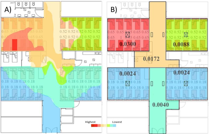
Figure 1: Small Droplet Transport and AIRC Box Model Approach Modified from Morawska and Milton (2020)

Figure 1 (A) illustrates the creation of an infectious droplet plume spreading throughout a poorly
ventilated room. Concentrations are higher closer to the emission source and decay moving further
away and will reach a pseudo steady-state profile in time if conditions are held approximately constant.
Figure 1 (B) shows the corresponding completely mixed box model for this scenario, where the
concentration in time becomes uniform across the room, and susceptible individuals are therefore
exposed to the same concentration regardless of their position in the room. Differences in exposure risk
between susceptible occupants in the room is therefore reduced to a function of exposure duration
rather than spatial location. Figure 1 (C) shows the conceptual effect of increasing the ventilation rate in
the room. The plume is reduced in intensity and extent, and the susceptible occupant is exposed to
lower viral concentrations and consequentially has reduced infection risk. Figure 1 (D) illustrates the
completely mixed box model approach for the room with improved ventilation. The susceptible
occupant is exposed to a lower concentration and thus has a lower probability of infection for the same
exposure time.
With the box model simplification, it becomes straightforward for AIRC to calculate changes in room
concentration over time. Depending on the strength and duration of the emission rate and the
ventilation rate in the room, the viral droplet concentration profile versus time will assume a predictable
curve shape. Three common concentration curves are presented in Figure 2.

Figure 2: Common concentration versus time curves for different contaminant source scenarios on a linear scale,
based on concept presented in NEEC (2015). Figure 2 (A) represents the concentration profile in a room with a
constant emission source and constant ventilation rate, showing how the concentration approaches a steady-state
asymptote. Figure 2 (B) presents a scenario where the same emission is eliminated and concentrations decay
accordingly due to constant ventilation. Figure 2 (C) shows a more dynamic scenario where there are two
separate, non-overlapping emission periods, with the second period resulting in higher concentration either due to
a higher emission rate or a lower ventilation rate.

With its simplifying assumptions, the accuracy and utility of AIRC becomes a question of scale. In
general, the smaller the enclosed space and the more completely mixed the air, the more the results will
approximate reality. An upper limit to the appropriate room size for AIRC cannot be definitively
provided at this time, but applications to indoor spaces that are thousands of square meters in area with
complex HVAC zoning are unlikely to produce useful risk predictions. Alternatively, a room of
approximately 500 square meters or less comprising a single HVAC zone is more likely to be a good
candidate for AIRC application. A practical way to accommodate larger buildings or spaces with complex
zoning is to divide the area into sub-zones, each represented by an AIRC model. The process is
conceptually illustrated in Figure 3, which depicts a multi-zone modeling approach to characterize the
March 2003 outbreak of SARS-CoV-1 in Ward 8A at the Prince of Wales Hospital in Hong Kong (Li et al.,
2005 and Xiao et al., 2017).

Figure 3: Simulated infectious aerosol distribution using a complex CFD model (A) and a simplified multi-zone
approach (B), modified from Xiao et al., 2017. Predicted aerosol concentrations for each approach are overlaid on
top of the reported SARS-CoV-1 attack rate in the zone. The index patient was located in the top left zone.

Figure 3 (A) presents a more realistic spatial representation of aerosol distribution, characterized by a
plume emanating from the index patient. However, the multi-zone approach on Figure 3 (B) is likely
sufficient to calculate infection risk, especially where conservative assumptions are used. Wagner et al.
(2009) takes a similar approach by implementing a Sequential Box Model (SBM) that incorporates air
exchange between zones.

Retrospective assessments of the AIRC risk modeling approach are provided in Buonanno et al. (2020b),
simulating the outbreaks of SARS-CoV-2 at a restaurant in Guangzhou, China and a choir rehearsal in
Skagit, WA, USA. The ability of the AIRC approach to reasonably reproduce these airborne
“superspreading events” indicate its validity for risk screening purposes, especially when considering the
urgent and time-critical need for quantitative tools to inform decision making during the SARS-CoV-2
pandemic. Furthermore, as noted in Buonanno et al. (2020a), in epidemic modeling quantifying
community transmission, it is impossible to specify the geometries, the ventilation, and the locations of
all infectious sources in each microenvironment. Therefore, adopting the completely mixed box model
approach is generally more reasonable than hypothesizing about myriad complex environments because
results must be interpreted on a statistical basis (Sze To and Chao, 2010).

SECTION III: THE INFECTION RISK MODEL
The detailed modeling approach implemented in AIRC and described in this section directly follows from
Buonanno et al. (2020a) and Buonanno et al. (2020b).

The model used to quantify airborne infection risk in AIRC was developed by Gammaitoni and Nucci
(Gammaitoni and Nucci, 1997), and was successfully applied in previous papers estimating the infection
risk due to different diseases (e.g. influenza, SARS, tuberculosis, rhinovirus) in various settings such as
airplanes (Wagner et al., 2009), cars (Knibbs et al., 2011), and hospitals. The model calculates the
quanta concentration (n) in an indoor environment over time, subject to a constant quanta emission
rate and removal rate. As a reminder, a quantum is the dose of airborne droplet nuclei required to
cause infection in 63% of susceptible persons (Buonanno et al., 2020a). The full equation for n(t),
including an initial concentration term (n0), is presented below:

 − ⦁ 
 ⦁ 
 ( ) ( ) = 0 + (1 − − ⦁ )
 3 ⦁ 
where IVRR (hr-1) represents the total infectious viral removal rate, I is the number of infectious subjects,
V is the volume of the indoor air environment, and ERq is the abovementioned quanta emission rate
(quanta/hr) characteristic of the specific disease/virus under investigation. The IVRR term is the sum of
three contributions, all expressed in hr-1: the air exchange rate (AER) via ventilation (typically measured
in the number of air changes per hour), the particle deposition rate on surfaces (k, e.g. via gravitational
settling), and the viral inactivation rate (λ) (Yang and Marr, 2011). Details on specification of these
three parameters are provided in Section IV.

In addition to the constant ERq and IVRR values, it is assumed that the latent period of the disease is
longer than the time scale of the model, and the droplets are instantaneously and evenly distributed in
the room, using the box model approach described in Section II (Gammaitoni and Nucci, 1997). Once
again, the latter represents a key assumption for the application of the model as it considers that the air
is well-mixed within the modelled space. The risk associated with an exposure is dependent on the dose
of quanta and duration of exposure, as well as the probability of occurrence of this exposure condition.
The dose of quanta (Dq) received by a susceptible subject can be obtained by integrating the calculated
quanta concentration over the total exposure time (T), as follows:

where IR is the inhalation rate of the exposed subject (m3/hr) which is a function of the subject’s activity
level. To determine the probability of infection (PI, %) of exposed susceptible occupants for a fixed ERq,
a simplified exponential dose-response model is used as presented below:

 26

The probability of infection assumes different values based on the selected quanta emission rate. As
such it is defined as a conditional probability for a discrete quanta emission rate, or PI(ERq). To evaluate
the individual risk (R) of an exposed person for a given exposure scenario, the probability of occurrence
of each ERq value (PERq), which is defined by an ERq probability density functions (pdfERq), must also be
evaluated. Since the probability of infection (PI(ERq)) and the probability of occurrence PERq are
independent events, the individual risk for a given ERq, R(ERq), can be evaluated as the product of the
two terms:

� �(%) = � � ∙

where PI(ERq) is the conditional probability of the infection, given a certain ERq, and PERq represents the
relative frequency of the specific ERq value. The individual risk (R) of an exposed person, considering the
full spectrum of possible ERq values within a defined distribution, can then be calculated by integrating
the pdfR for all possible ERq values, i.e. summing up the R(ERq) values as follows:

(%) = � � � = � � � � ∙ �

The individual risk R also represents the ratio between the number of infection cases (C) and the
number of exposed susceptible individuals (S) for a given exposure scenario and taking into account all
possible ERq values for the infectious subject under investigation (Buonanno et al., 2020b). In
retrospective analyses of documented outbreaks, the known C/S ratio is typically defined as the “attack
rate”.

New to Version 2.0, AIRC includes a stationary exposure conditions model (“AIRC SEC”) that fully
implements the above method to calculate individual risk taking into account all possible ERq values for
an assumed infectious occupant activity. However, where the room ventilation, volume, subject
activity, etc. are treated as constant values, Buonanno et al. (2020b) shows that a simplified estimate of
R can be calculated by using the ERq value assumed with a probability of occurrence PERq=1 (i.e.
considered as a certain emission) which induces a PI(ERq) equal to the risk R as shown through the full
integration analysis. This certain emission value is calculated to be the 66th percentile ERq value.
Therefore, when the 66th percentile ERq value is used, the individual risk can be assumed to
approximately equal to the probability of infection. AIRC therefore provides the 66th percentile values
for a range of respiratory activities and recommends these values to be used in risk calculations for the
AIRC Version 1.0 update with transitional exposure conditions, now termed “AIRC TEC” (Buonanno et al.,
2020b). [CHANGED TO 75th PERCENTILE {ADJUSTABLE} IN VERSION 3.0 BETA FOR NEW EMISSION
DISTRIBUTION WITH INCREASED OVERDISPERSION] The key distinction between AIRC SEC and AIRC TEC
is the type of exposure scenario being evaluated. AIRC SEC assumes perfect coincidence in the presence
of the two subjects as they enter together and leave the environment together. AIRC TEC allows
consideration of more dynamic scenarios where infectious and susceptible occupants can come and go
and different times, and susceptible occupants can be exposed to residual viral droplets in the air.
When the exact same scenario is evaluated using AIRC SEC and AIRC TEC, the results will be nearly
identical for short exposures (

On a population level, the basic reproduction number R0, representing the number of susceptible people
infected after the exposure time, can be determined by multiplying the probability of infection (PI, %) by
the number of exposed individuals. For purposes of AIRC, however, reproductive effects are calculated
differently to provide the maximum number of occupants that may keep the R0 below 1 for the scenario
in question. In this way the user can obtain a potential occupancy or crowding index that considers the
need to reduce community transmission. [CHANGED TERMINOLOGY TO EVENT REPRODUCTION
NUMBER]

This maximum occupancy calculation uses the following equation, rounded down to the nearest integer:
 1
 . 0 ( ) < 1 =
 ( )

For both AIRC SEC and AIRC TEC, the PI value corresponding to the 90th percentile ERq value is used as
the maximum R(ERq) values occur in the narrow range of 90th-95th percentile for the scenarios evaluated
by Buonanno et al. (2020b). [WITH THE IMPROVED EMISSION DISTRIBUTION THE MAXIMUM
OCCUPANCY IS NOW CALCULATED AS 1/R FOR THE SEC VERSION AND 1/PI FOR THE TEC VERSION]

 28

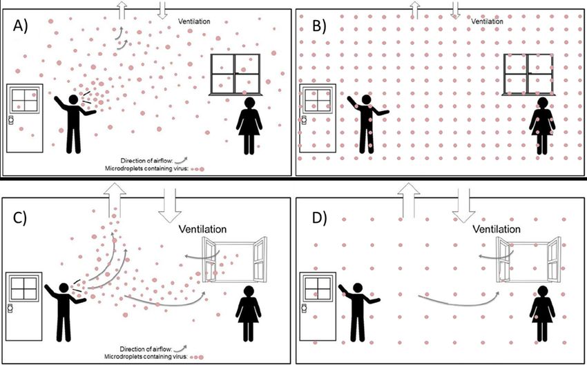
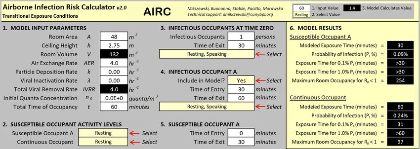
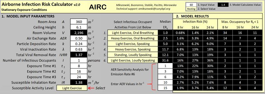
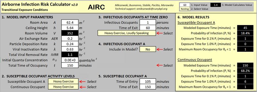
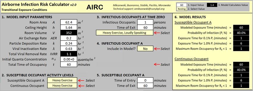
SECTION IV: AIRC DATA ENTRY & RESULTS
There are two tabs for the user to enter data in AIRC and view model output, the first tab entitled “AIRC
SEC” (new to Version 2.0) and the second tab entitled “AIRC TEC”. These two modeling sheets are
completely independent. If a user is only interested in one approach, the other one can be ignored. For
both sheets the user must enter a value into all cells with white fill and black text. All cells with black fill
and white text are calculated by AIRC and are locked to the user. Cells with gray fill are informational
and are not used by AIRC. In addition, drop-down lists in cells with yellow fill are used on both tabs to
select the desired activities for infectious and susceptible occupants. Based on the assumption that
users are most concerned with SARS-CoV-2, quanta emission rates associated with the selected
activities are for SARS-CoV-2. These values are defined on the “SEC Calculations” tab and the “TEC ERq
IR” tabs for the two different modeling approaches.

A description of each tab in the AIRC 2.0 workbook is provided below. All tabs associated with AIRC SEC
are shaded blue, all tabs associated with AIRC TEC are shaded yellow.

AIRC SEC Tabs

AIRC SEC Tab 1 Name: AIRC SEC

Description: This tab contains model input and results for the constant source and exposure, termed
“stationary exposure conditions” model (SEC) new to AIRC Version 2.0. The individual infection risk and
maximum room occupancy is calculated for six different selectable infectious occupant activities for
three different exposure lengths. In addition, a sensitivity analysis on the air exchange rate parameter is
presented for one infectious occupant activity where the user can enter five different air exchange rates
to see how model results change.

Model Input Parameters:

1. Room Dimensions

The room dimension parameters for the user to enter are the floor plan area (in m2) and the ceiling
height of the occupied indoor space to be modeled (in m). The product of the area and ceiling height is
the room volume (m3).

2. Infectious Viral Removal Rate

As defined in Section III, the Infectious Viral Removal Rate (IVRR) is the sum of the air exchange rate
(AER) via ventilation (also termed the number of air changes per hour), the particle deposition rate on
surfaces (k, e.g. via gravitational settling), and the viral inactivation rate (λ). Entry details on these three
parameters are presented below.

Parameter Air Exchange Rate (AER)

Units hour (hr-1)

Recommended Values Use site-specific measured values, or design or estimated values if
 field measurements are unavailable. For natural ventilation
 (infiltration only), values of 0.2 – 0.5 hr-1 are recommended. For the
 opening of doors and windows on one side of a room, values of 1.0
 – 5.0 hr-1 are suggested. It is noted that ventilation rates through
 windows are highly site-specific and the user is cautioned against
 making assumptions on the higher end of this provided range.

Notes/Estimation The AER is the most important site-specific parameter in the
Methods model and the largest contributor to virus removal. Therefore,
 site-specific measurements or design values are the best sources
 for parameter input. AER can be simply calculated as the total
 fresh outdoor airflow (OA) divided by the volume of the room.
 Recirculated airflow should not be included in the AER calculation
 as it represents fresh airflow only.

 If actual total and outdoor airflows cannot be measured directly,
 the percent OA delivered to a space is commonly estimated using
 air handler carbon dioxide (CO2) concentrations in parts per million
 (ppm) as follows:

 Note that the above calculation is also routinely performed using
 temperatures instead of CO2 concentrations, but that it is less
 accurate, especially when temperature differences are small.
 Another common method of estimating ventilation rate is using
 “rule of thumb” values per person based on steady-state CO2
 concentrations achieved in offices and classrooms with ASHRAE
 62n default occupancy rates, as follows (NEEC, 2015):

 Zone CO2 Outside Air Outside Air Outside Air
 (ppm) (CFM per (Liters (L)/s (m3/hr per
 person) per person) person)
 2,500 5 2.4 8.5
 1,400 10 4.7 17
 1,000 15 6.9 25
 750 30 14 51

 30

AIRC follows the risk minimization framework outlined by
 Morawska et al. (2020), in which enhanced ventilation is the
 primary reliable and readily available line of defense against
 airborne transmission in indoor air environments. Secondary
 measures where ventilation alone may be insufficient, such as
 enhanced filtration, ultraviolet germicidal irradiation (UVGI),
 and/or room humidification, are not explicitly included in AIRC.
 Advanced users of AIRC can include filtration in the model by
 adding “equivalent” air exchanges to the AER term.

 Azimi and Stephens (2013) provide a comprehensive review of
 infectious droplet nuclei filtration efficiencies (see Figure 4). To
 incorporate filtration removal in AIRC, the user can calculate the
 equivalent AER in hr-1 as follows:

 where Qrecirculated is the airflow rate recirculated from the space
 through the filter, ƞfilter is the infectious droplet removal efficiency
 of the filter, and V is the volume of the room.

 The recirculated airflow plus the fresh outdoor airflow will equal
 the total airflow rate of the air handler. Remember that the air
 exchange rate is calculated using only the fresh outdoor airflow
 rate, and if air is recirculated the AER will be reduced. Example
 Application 3 presents how this calculation is performed for an air
 handler serving an office space.

Parameter Particle Deposition Rate (k) (SARS-CoV-2)

Units hr-1

Recommended Value 0.24

Notes/Estimation The recommended value is from Buonanno et al. (2020a), which
Methods calculated the deposition rate as the ratio between the settling
 velocity of super-micrometric particles (roughly 1.0 × 10−4 m s−1 as
 measured by Chatoutsidou and Lazaridis [2019]) and the height of
 the emission source (1.5 m). A site-specific computational fluid
 dynamics (CFD) model may be needed to quantify this parameter
 more accurately.

 31

Parameter Viral Inactivation Rate (λ) (SARS-CoV-2)

 Units hr-1

 Recommended Value 0.63

 Notes/Estimation The recommended viral inactivation rate is calculated from the
 Methods SARS-CoV-2 half-life (1.1 hr) detected by van Doremalen et al.
 (2020) as follows:

 Users should follow the evolving literature on SARS-CoV-2 with a
 view towards refinement of this parameter. Fears et al. (2020)
 reports retained infectivity and virion integrity of SARS-CoV-2 for
 up to 16 hours in respirable-sized aerosols. For a resource to help
 incorporate UV treatment or relative humidity into this parameter,
 the user is referred to: https://www.dhs.gov/science-and-
 technology/sars-airborne-calculator (Schuit et al., 2020).

Figure 4: Infectious droplet nuclei filtration efficiency (ƞfilter) as a function of HVAC filter MERV rating, using the
 minimum reported values from Azimi and Stephens (2013).

 32

3. Number of Infectious Occupants

New to Version 2.0, the user can model infectious occupants as a group of multiple individuals in the
room for the same defined period of time. For AIRC SEC, the infected group is in the room for the full
length of the simulation with the susceptible individuals. Any positive integer may be entered for this
value. [NOW SELECTABLE FOR UP TO 10 INFECTIOUS OCCUPANTS]

4. Initial Quanta Concentration

The initial quanta concentration term, in quanta/m3, has been provided in the event the user wants to
model a scenario where residual viral emissions are present in indoor air at time zero. This is a useful
function where the user wants to begin a new simulation using the final quanta concentration of a
previous simulation. If the indoor air environment is expected to be free of airborne virus at the start of
the simulation, the user should enter zero for this parameter.

5. Exposure Time

AIRC SEC calculates infection risk and maximum occupancy for three different exposure times that the
user can enter in hours (with no time limit).

6. Susceptible Inhalation Rate

The user can select from a list of pre-determined activity levels (resting, standing, light exercise, heavy
exercise) to quantify the inhalation rate of susceptible occupants in the model. If a user would like to
enter a custom inhalation rate value, this may be done on the SEC Calculations tab.

7. Infectious Occupant Activities

The user can select six (6) different pre-determined activity levels from the list provided in Table 1 to
quantify the viral emission rate (ERq) of infectious occupants of the room, from Buonanno et al. (2020b).

Table 1: Selectable Infectious Occupant Activities and Associated ERq Values
[SUPERCEDED – SEE ‘ERQ’ TAB OF VERSION 3.0 BETA FOR UPDATED DISTRIBUTIONS FOR SARS-COV-2
AND OTHER PATHOGENS]

The results represent six different model realizations for the same scenario, not different infectious
occupants doing different things in the same room. This can be conceptualized as a sensitivity analysis
on the selected ERq distribution for the model. If a user would like to enter a custom ERq distribution or
a fixed ERq value for use in the model, this may be done on the SEC Calculations tab.

8. AER Sensitivity Analysis

To help the user assess how model results change based on air exchange rate, the user may enter five
different AER values that will re-calculate results for infectious occupant activity #6 only.

9. Model Results

This section presents the model results as the individual infection risk for exposed susceptible occupants
for the three different exposure times, and as the estimated maximum number of occupants to maintain
a reproductive number less than one for the modeled scenario. In total the results reflect 33 different

You can also read