The Heliospheric Ambipolar Potential Inferred from Sunward-Propagating Halo Electrons

MNRAS 000, 1–10 (2022) Preprint 19 April 2022 Compiled using MNRAS LATEX style file v3.0

 The Heliospheric Ambipolar Potential Inferred from
 Sunward-Propagating Halo Electrons
 Konstantinos Horaites,1★ Stanislav Boldyrev2,3
 1 Department of Physics, University of Helsinki, Helsinki, Finland
 2 Department of Physics, University of Wisconsin–Madison, Madison, WI 53706, USA
 3 Center for Space Plasma Physics, Space Science Institute, Boulder, CO 80301, USA
arXiv:2204.06532v2 [physics.space-ph] 18 Apr 2022

 Accepted XXX. Received YYY; in original form ZZZ

 ABSTRACT
 We provide evidence that the sunward-propagating half of the solar wind electron halo distribution evolves without scattering
 in the inner heliosphere. We assume the particles conserve their total energy and magnetic moment, and perform a “Liouville
 mapping” on electron pitch angle distributions measured by the Parker Solar Probe SPAN-E instrument. Namely, we show that
 the distributions are consistent with Liouville’s theorem if an appropriate interplanetary potential is chosen. This potential,
 an outcome of our fitting method, is compared against the radial profiles of proton bulk flow energy. We find that the inferred
 potential is responsible for nearly 100% of the proton acceleration in the solar wind at heliocentric distances 0.18-0.79 AU. These
 observations combine to form a coherent physical picture: the same interplanetary potential accounts for the acceleration of the
 solar wind protons as well as the evolution of the electron halo. In this picture the halo is formed from a sunward-propagating
 population that originates somewhere in the outer heliosphere by a yet-unknown mechanism.
 Key words: solar wind – plasmas

 1 INTRODUCTION et al. 2020). The estimated polarization potential between the exobase
 (∼0.01-0.05 AU) and 1 AU is on the order of 100-1000 eV.
 Electrons in the solar wind occupy different collisional regimes, de-
 pending on their energy. The typical frequency of Coulomb collisions Despite the general acknowledgment of a large-scale electro-
 experienced by a test particle is known to fall off precipitously with static field’s presence in the solar wind, the magnitude of this field
 the particle’s speed (as −3 ). At low energies .10 eV, collisions ( ∼10−9 V/m) is far too small to be measured directly by spacecraft.
 help to shape the electron velocity distribution function (eVDF) into However, recent progress has been made by considering the impact
 a Maxwellian “core”. But the so-called “suprathermal” electrons, of the electric potential on the eVDF. In Berčič et al. (2021b), abbre-
 which have speeds much greater than the thermal speed, largely ig- viated here as B21, the ambipolar potential was indirectly inferred
 nore their binary electrostatic interactions with nearby charged parti- from eVDFs measured by the Parker Solar Probe (PSP) SPAN-E
 cles. It is frequently appropriate to treat the suprathermal electrons as electron instrument (Whittlesey et al. 2020). These measurements
 “collisionless”, so that their motion is only guided by the collective are based on two signals associated with the large-scale potential:
 fields in the plasma. The influence of these fields on the particles 1) the “deficit” of sunward-moving electrons in the Maxwellian core
 can be loosely separated into two categories: the acceleration by (Halekas et al. 2020, 2021), and 2) the “breakpoint energy” (Scudder
 large-scale fields and scattering by wave-particle interactions. & Olbert 1979; Bakrania et al. 2020) that delineates the core from
 The rapid escape of electrons to large heliospheric distances es- the suprathermal electrons. In B21, this theory was applied to PSP
 tablishes an equilibrium where the near-sun environment has a slight data to infer a parallel electric field k with a typical magnitude
 excess of positive charge. The resulting large-scale “ambipolar” or ∼10−9 V/m and scaling with heliocentric distance k ∝ −1.69 . As
 “polarization” electric field radially accelerates the solar wind ions, reported, a solar wind accelerated by such a field would have 59% of
 which then drag the electrons along. This field was not considered the energy (77% of the speed) predicted by exospheric models at 45
 explicitly in the earliest hydrodynamic models of the solar wind solar radii ( ). The remaining energy however presents a significant
 (e.g., Parker 1958). But it was gradually incorporated into the theory, gap between these observations and theory.
 where for instance it features prominently in so-called “exospheric” Although the results described above demonstrate a strong con-
 or kinetic models (e.g., Sen 1969; Jockers 1970; Lemaire & Scherer nection between the potential and the electron distribution, some lim-
 1971). In these kinetic models, particles abruptly become collision- itations of the core deficit method can be recognized. The detailed
 less above the “exobase” (e.g., Zouganelis et al. 2004; Boldyrev physics governing the Maxwellian core distribution is complex, as
 the solar wind electrons are weakly collisional (Knudsen number
 &0.01), and exhibit large plasma gradients (e.g., Bale et al. 2013).
 Such a kinetic regime is difficult to treat with standard methods (e.g.,
 ★ E-mail: konstantinos.horaites@helsinki.fi Spitzer & Härm 1953; Gurevich & Istomin 1979). This is before

 © 2022 The Authors

2 K. Horaites et al.
consideration of instabilities that may affect the core (e.g., Schroeder shift directly corresponds with the ambipolar potential itself. We will
et al. 2021), which may even be generated by a resonant interaction therefore perform a “Liouville mapping” (e.g., Schwartz et al. 1998;
with the deficit electrons themselves (Berčič et al. 2021a). Thus the Lefebvre et al. 2007) to infer the potential from the eVDFs as ob-
authors of B21 caution that their approach is “simplified and includes served by Parker Solar Probe in the inner heliosphere 0.18–0.79 AU
strong assumptions”, and may cause either a systematic overestima- (39–170 ).
tion or underestimation of the potential depending on how the method We will demonstrate that a single Liouville mapping can be applied
is applied. The core deficit in particular is not clearly described theo- to accurately model the halo eVDFs over a broad range of distances.
retically, as this subtle feature is simply identified with the “electron Moreover, we will show that the ambipolar potential inferred from
cutoff” (a sharp discontinuity) in the sunward eVDF that is seen in the eVDFs is exactly that required to accelerate the solar wind protons
exospheric models. Without more detailed predictions, the deficit can over these distances. This creates a coherent physical picture in which
only be measured with a heuristic approach. The core perturbation the same electric field causes two independently measurable trends
has only been detected in 57% of eVDFs at heliospheric distances as heliocentric distance increases: the halo loses energy while the
20–85 . This fractional occurrence decreases at the larger radial bulk proton flow accelerates.
distances occupied by most spacecraft.
 In the current work, we develop a method that complements the
pioneering study of B21 by considering the effect of the large-scale 2 THEORY
potential on a different part of the electron distribution: the suprather-
mal “halo” population. The halo is identified in solar wind eVDFs as The Vlasov equation describes the evolution of the distribution func-
a nearly-isotropic tail at energies ∼100-1000 eV (e.g., Feldman et al. tion (x, v, ) for a particle species in the absence of diffusion:
1975; Pilipp et al. 1987). As the halo energies are comparable to
predictions for the inner heliospheric potential, this potential should 
 + v · ∇ + a · ∇ = 0, (1)
profoundly affect the eVDF. 
 In the present work we neglect the processes that generate the halo, where a(x, ) represents the acceleration due to the forces (Lorentz,
but this topic deserves some review. Notably, the apparent growth of gravitational) that act on the particles. Equation 1 neglects both
the halo at the expense of the anti-sunward suprathermal “strahl” Coulomb collisions and wave-particle interactions. The general so-
population may imply that the halo is locally formed in the inner lution, known also as Liouville’s Theorem, states that is constant
heliosphere by scattered strahl electrons (e.g., Maksimovic et al. along the particle trajectories:
2005; Štverák et al. 2009). This has led to significant theoretical
development, focused on the resonant interaction of electrons with
the whistler and fast-magnetosonic whistler (FM/W) modes (e.g., (x( ), v( ), ) = (x0 , v0 , 0 ), (2)
Vocks et al. 2005; Saito & Gary 2007; Vasko et al. 2019; Verscharen In eq. 2, the coordinates x( ), v( ), describes the time-dependent
et al. 2019b; Micera et al. 2021; Zenteno-Quinteros et al. 2021; Vo motion of an arbitrary particle with initial position x0 = x( 0 ) and
et al. 2022; Tang et al. 2022). Observations have struggled to confirm velocity v0 = v( 0 ), under the acceleration v/ = a(x( ), ).
these theories. Notably, whistlers are practically absent (occurrence Liouville’s Theorem (2) is especially useful when the particle
rate 0.8 AU), charge. Note that in eq. 3 the Sun’s gravitational potential is ignored,
as it is natural for highly energetic sunward-moving particles to orig- as the gravitational energy of an electron at 1 AU is 1 eV.
inate from larger distances. From the considerations detailed above, In the solar wind we expect the large scale gradients / 

The Heliospheric Ambipolar Potential Inferred from Sunward-Propagating Halo Electrons 3
 sin2 = sin2 (180◦ − ), which would complicate the notation. We
 also treat the “passing” and “reflected” populations (e.g., Lefebvre
 et al. 2007) equally, as the distinction is not of great importance here.
 Frequently, one wishes to map the eVDF from one location to
 another. Let us suppose that at a given position ★ the functional
 form of the eVDF, ★ ( , ), is known:

 ★ ( , ) ≡ ( ★, , ). (7)
 Then, the solution ( , , ) is constructed by repeatedly substi-
 tuting the definitions (3), (4) of the invariants into the boundary
 condition (7):

 ( , , ) =
 √︄
  (8)
 ( ★) sin2 
 
 ★
 − Δ ( , ★) , sin−1
 ( )( − Δ ( , ★))
 ,

 φ(r )> φ(rB) where we have introduced the notation Δ ( , ) to represent the
 potential difference between distances and ,
 B(r )> B(rB)
 Δ ( , ) ≡ ( ) − ( ). (9)

 sun θ It can be verified by inspection that the mapping formula (8) has the
 form (6) required by Liouville’s theorem and satisfies the boundary
 condition (7). The arguments of the 2D function ★ in (8) are the
 formulas for how K, of a given electron respectively map across
 distance under the constraints E=const., =const. Technically, our
 B Liouville mapping is derived for eVDFs measured simultaneously
 A
 along the same field line, but we ignore this detail by assuming the
 solar wind in the ecliptic is steady-state and cylindrically symmetric.
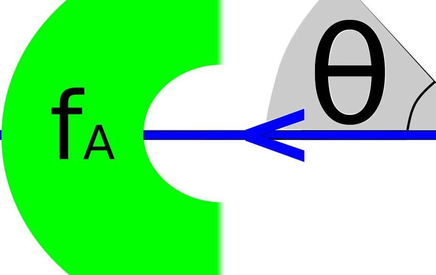
Figure 1. As a consequence of Liouville’s theorem, an initial halo electron From equations 6, 8 it is readily seen that if the halo eVDFs
distribution at position will distort as the particles migrate towards the are measured at two different distances along with the local magnetic
Sun along a field line (blue). This process is shown schematically. The green
 field , the only unknown variable is the potential . With an accurate
wedge-shaped region of the velocity distribution (imagined in k , ⊥ space)
maps to the distribution . The mirror force causes broadening, while the
 determination of , a function of the form (6) can be found that
changing potential causes the electrons to gain energy. The red regions of matches two (or more) such eVDFs. Such a “Liouville mapping”
represent particles that will be reflected by the magnetic field before arriving may be accomplished with statistical methods (see sections 3.1, 3.2)
at . The white semicircular vacancies in , are the domain of the and constitutes a measurement of the potential. In section 3 we apply
collisional core distribution, not considered here. a Liouville mapping to the average eVDFs measured by PSP, to infer
 the potential ( ) in the inner heliosphere.

 Note that the 2D velocity space of the distribution may be writ-
ten in terms of many sets of variables, e.g., { ⊥ , k }, { , cos },
 3 OBSERVATIONS
or { , }. In the context of Liouville’s theorem it is often conve-
nient to use {E, }. For the purpose of comparison with spacecraft Our primary data set comes from the SPAN-E electron experiment,
measurements, in this work we will primarily use { , }. a pair of electrostatic analyzers (ESAs) onboard the PSP satellite
 As discussed above, conservation of E, leads to a general so- (Whittlesey et al. 2020). SPAN-E is part of the Solar Wind Electrons
lution to the steady-state ( / =0) Vlasov equation (1) for the halo Alphas and Protons (SWEAP) investigation (Kasper et al. 2016).
electrons: Each SPAN-E ESA has a nominal field of view (FOV) of 240◦ ×120◦ ,
 but the instruments are arranged in a complementary fashion so that
 together they observe >90% of the sky after considering physical ob-
 = ˜(E, ). (5)
 structions such as the spacecraft heat shield. We studied the Level 3
Given such a function ˜, the solution ( , , ) can be written im- pitch angle distribution (PAD) data, which were generated by col-
mediately by substituting the definitions (3), (4) into (5): lating the 3D eVDFs measured by the two ESAs into 2D ( , )
 distributions. The pitch angle is determined in the Level 3 data by
 referencing the FIELDS fluxgate magnetometer (Bale et al. 2016).
  sin2 
 ( , , ) = ˜ − ( ), . (6) Each PAD has 12 evenly spaced pitch-angle bins (15◦ wide each)
 ( ) and 32 energy bins logarithmically spaced over a range ∼2–1800 eV.
In terms of the variables , , , Liouville’s theorem requires that Such PADs are appropriate for the study of solar wind halo, as the
any solution for should be of the form (6), which just restates halo electrons are gyrotropic and have typical energies 100-1000 eV.
that is a function of the total energy and the magnetic moment. We considered available Level 3 SPAN-E observations (∼10 −
For simplicity we will only consider sunward-directed electrons, i.e. 20 second cadence) between the dates October 31, 2018 and De-
 ∈ [0◦ , 90◦ ]. This avoids accounting for the phase-space redundancy cember 31, 2020. This time range is centered approximately around

 MNRAS 000, 1–10 (2022)

4 K. Horaites et al.
the solar minimum associated with the onset of Solar Cycle 25. eddy turnover time in the slow solar wind (Weygand et al. 2013),
During this time period the PADs are only available irregularly, i.e. the time-scale over which successive measurements become un-
but as the spacecraft completed multiple orbits there is sufficient correlated. We assume that 4-hour averages of solar wind data are
coverage of the distances 0.18-0.79 AU (i.e. each distance is sam- independent and identically distributed (i.i.d.). This allows error bars
pled by a few orbits). We remove data associated with co-rotating of the distance-averaged PADs to be computed from the standard
interaction regions (CIRs) and stream interaction regions (SIRs) en- deviation of the mean. We expect i.i.d. is a coarse approximation
countered by PSP, as indexed by Allen et al. (2021). Coronal mass as PSP measurements are affected by many processes on different
ejections (CMEs) encountered by PSP are also removed using the timescales, e.g. turbulence (hours or less), data gaps (days), and solar
HELIO4CAST ICMECAT list (Möstl et al. 2020). Guided by the rotation (weeks). The solar cycle, which occurs over an 11-year pe-
criteria in Nieves-Chinchilla et al. (2018), it contains only ICME riod, is unlikely to affect our analysis since our data are all measured
events that show clear signatures of magnetic obstacles. This helps near solar minimum.
for instance to avoid contamination by the “counterstreaming” strahl, Energy cuts of the resulting distance-averaged PADs are shown in
which is a sunward-directed electron beam that is frequently seen Figure 2, for different distances. The energy cuts of the distribution
during the passage of CMEs (Gosling et al. 1987, 1992). Measure- are taken from the most field-aligned sunward pitch angle bin of the
ments taken while SPAN-E’s mechanical attenuator was deployed PAD (0◦

The Heliospheric Ambipolar Potential Inferred from Sunward-Propagating Halo Electrons 5
 the most field-aligned cut of the eVDF (representing 0◦ < 

6 K. Horaites et al.
 all data shown in the 8 panels. We calculate a reduced chi-squared
 value of 2 / = 1.10 ( =172 degrees of freedom, p-value 0.16),
 which is statistically significant. It is especially noteworthy that our
 fit successfully matched the averaged PADs even though they have
 very small error bars. As our model function (13) is constrained
 to comply with Liouville’s theorem, we may infer that Liouville’s
 theorem is consistent with the halo PAD data.
 To further investigate the significance of our results, we checked
 fB fA whether the collisionless model (13) could represent the strahl (which
 f is superficially similar to the halo) equally well. This amounted
 to repeating our 2D fit method, but redefining the pitch angle:
 ΔK → (180◦ − ). This way, the fit domain ∈ [0◦ , 90◦ ] corresponded
 to the anti-sunward half of the eVDF. The converged fit (not shown)
 clearly did not match the strahl data, and resulted in an unacceptable
 reduced chi-squared value: 2 / =20.1 ( =171 degrees of freedom,
 p-value ≪1). Of course, it is well-known that scattering (Coulomb
 collisions and/or wave-particle interactions) is required to explain
 the strahl angular width (e.g., Lemons & Feldman 1983), so it is
 expected that the model function (13) cannot explain the radial varia-
 K tion of the strahl. But this illustrates that Liouville’s theorem is highly
 restrictive—it cannot be satisfied by arbitrary eVDF data.

 Df(r1,r6), 1D Method
 3.3 Proton Acceleration
 -17
 10 The large-scale ambipolar potential is known to accelerate the solar
 wind proton flow. In the approximation that the potential in the eclip-
 tic is cylindrically symmetric and the protons flow radially outward,
 a change in potential corresponds directly to a change in radial flow
 speed. If the ambipolar potential changes with distance as we have
 -18
 10
f [m s ]

 inferred from the halo eVDFs (Sections 3.1, 3.2), then the proton
-6 -3

 flow energy should change by the same magnitude (up to a small
 correction due to gravity).
 To test this hypothesis, we examine the measurements of the pro-
 ton flow speed made by SWEAP’s SPC Faraday cup. We use the
 -19
 10 Level 3 velocity data, where for each SPC ion distribution a single
 1-dimensional Maxwellian fit was applied in the inertial RTN frame.
 From this fit we can extract the radial ("R") component of the proton
 velocity . We then compute the kinetic energy of the proton flow:
 Df=174.8±10.4
 = 2 /2, where is the proton mass. The measurements of
 -20
 10 0 100 200 300 400
 are averaged into 4-hour intervals and subsequently averaged by
 distance, as was done with the electron PADs. This gives a proton
 DK [eV] energy measurement ( ) at each distance (see Table 1).
 Because the protons (here treated as a mono-energetic beam) con-
 serve their total (kinetic+potential) energy, the change in electric
Figure 3. Top: In the 1D method (section 3.1), interpolation between two potential Δ is given by the formula:
sunward-directed ≈0◦ halo cuts at fixed phase space density (y-axis) yields
a set of measurements Δ of the energy shift (dashed lines). These are used
to estimate the potential difference Δ ( , ) between the distances , Δ ( 1 , ) = Δ ( ) + ΔΦ ( ), (15)
 . Bottom: An example of the 1D method applied to our PAD data, showing
measurements of the energy shift Δ (blue dots) between the 1 ≈0.2 AU and where we have defined Δ ( ) and ΔΦ ( ) as the changes in
 6 ≈0.5 AU cuts. A weighted average of the Δ (eq. 11) yields the potential kinetic and gravitational potential energy, relative to the innermost
difference Δ ( 1 , 6 )=174.8±10.4 eV. The final results for the 1D method distance 1 :
potentials, Δ ( 1 , ) for each , are shown in Table 1.

 Δ ( ) ≡ ( ) − ( 1 ), (16)

The Heliospheric Ambipolar Potential Inferred from Sunward-Propagating Halo Electrons 7

Figure 4. Halo electron pitch angle distributions (0◦ < < 90◦ , bin width Δ =15◦ ) measured by SPAN-E, averaged at =8 distance 1 , 2 , ... 8 . Each panel
represents a different distance, and different cuts of constant energy are distinguished by color. We considered PAD data in the energy range [391,935] eV and
phase space densities within [2e-20,1e-17] m−6 s3 . A single non-linear least squares fit is performed to all data shown (fit parameters listed in Tables 1, 2). The
fit uses a flexible model equation (13), a 2D polynomial that is constrained to satisfy Liouville’s theorem. The electron energization Δ manifests in these plots
as a vertical translation in phase space density of a given energy cut (color) between distances (panels).

 MNRAS 000, 1–10 (2022)

8 K. Horaites et al.
 tial ∼270 eV causes the halo electrons to lose this same amount of ki-
 Proton Bulk Speed netic energy, while the total (electric+gravitational) potential causes
 600 the protons to gain ∼230 eV in bulk flow energy. In terms of velocity,
 on average the protons start with radial speeds ≈290 km/sec at
 4-hour data 0.18 AU and increase to ≈360 km/sec at 0.79 AU.
 Distance avg.
 500
vp [km/sec]

 400

 300 4 DISCUSSION
 It is appropriate to compare our measurements of the potential with
 the results of B21. In that work, the authors report that the large-scale
 200 potential varies as ( ) = Φ0 ( / ) Φ in the interval 0.1. .0.4
 0.1 1.0 AU. They report two pairs of fit parameters: {Φ0 =1556.64 V, Φ =-
 r [AU] 0.66} and {Φ0 =1043.88 V, Φ =-0.55}. From these profiles we cal-
 culate the change in potential Δ ( 1 , ), which we plot for com-
 Energy Change w.r.t. r=r1 parison as dashed/dotted lines in Figure 5. The B21 profiles agree
 300 roughly with our measurements of eΔ in the interval where both

 DKp + DFG
 techniques were applied (0.2-0.4 AU). The error bars, however, are
 comparable to the signal for these small energies (. 50 eV). We note

 eDf (1D)
 that in our measurements Δ changes by >100 volts in the interval
 200 [0.4,0.8] AU, while extrapolation of B21 yields only Δ ≈30–40 volts
 eDf (2D)
Energy [eV]

 over this same interval. An increase of hundreds of volts between 0.2
 and 0.8 AU is not at all unreasonable in the slow wind. Such an
 100 increase may indeed be expected for the protons to accelerate from
 their modest ∼300 km/sec speeds observed at 0.2 AU to their typical
 B21 ∼1 AU values ∼400km/sec (McGregor et al. 2011).
 Our results displayed in Fig. 5 indicate that the acceleration of the
 0 slow solar wind is almost entirely due to the ambipolar electric field.
 Gravity is found to have a significant impact as well, and should
 increase in importance near the Sun (Lamy et al. 2003). In the same
 -100 sense, gravitational forces diminish rapidly with distance and may
 0.1 1.0 be entirely neglected in the outer heliosphere. As may be seen from
 r [AU] Ulysses measurements (e.g. Štverák et al. 2009), the halo itself does
 evolve slowly in the outer heliosphere. This evolution could be due
 Figure 5. Top: The 4-hour averages of the radial proton bulk speed ,
 in part or in whole to the radial variation of the ambipolar potential.
 as measured by the SPC Faraday Cup, are shown as circles. The red line
 shows the average binned by distance (at ). The data show a steady The Liouville mapping technique accurately describes the halo
 increasing trend, except the dip around 4 ≈0.34 AU, which we treat as an eVDF. This implies that halo electrons are not affected by diffusive
 outlier. Bottom: The change in electric potential Δ ( 1 , ) inferred in two wave-particle interactions in the inner heliosphere. This is in itself
 different ways: 1) from the change in proton kinetic energy Δ , correcting an important result, as many theories of halo generation presuppose
 for gravity (red, eq. 15), and 2) from the electron halo via the 1D (green) some local wave mechanism, that for example could scatter the strahl
 and 2D (blue) methods. The two independent estimations of the potential population into the halo. However, the absence of halo and/or strahl
 agree within the error bars. The change in potential is given with respect diffusion is consistent with the recent measurements of Cattell et al.
 to the minimum distance 1 =0.202 AU. Two lines are plotted 0.1-0.4 AU, (2022); Jeong et al. (2022a) which respectively show that whistler
 representing the variation of the potential Δ ( 1 , ) derived from B21, for
 and FM/W waves do not scatter the strahl near the Sun. Our results
 comparison (see text).
 do not preclude the occasional action of instabilities that derive their
 free energy from the halo particles, which have been observed e.g.,
 at 1 AU (Tong et al. 2019). But to zeroth order we may infer that
 energy cannot be completely neglected, as ΔΦ ≈40 eV across the the average sunward halo eVDFs observed by PSP are not locally
 distances 0.18-0.79 AU. affected by these instabilities.
 In Fig. 5, we compare the change in potential Δ ( 1 , ) as it If the sunward-moving halo electrons observed 0.18-0.79 AU are
 is calculated independently in two ways: 1) from the proton kinetic not produced locally by wave-particle diffusion, then they must have
 energy (corrected by gravity, eq. 15) and 2) from the halo eVDFs originated from some larger heliocentric distance. Such a mecha-
 (1D and 2D methods). The two estimates agree well at all distances nism of halo generation has not been deeply explored in the present
 0.18-0.79 AU, implying a change in potential Δ ∼270 eV over the body of research. However, as suggested in Horaites et al. (2019),
 entire interval. This agreement implies that the electric potential in- if a sunward-moving suprathermal population is formed in the outer
 ferred from the halo eVDFs fully explains proton acceleration over heliosphere, the process of magnetic mirroring should cause it to
 this distance interval. In rough numbers, the change in electric poten- appear nearly isotropic in the inner heliosphere.

 MNRAS 000, 1–10 (2022)

The Heliospheric Ambipolar Potential Inferred from Sunward-Propagating Halo Electrons 9
 range [ ] [AU] B( ) [nT] ( ) [eV] 1D Method: Δ ( 1 , ) [V] 2D Fit: ≡ Δ ( 1 , ) [V]
 [0.18, 0.21] 1 = 0.202 54.3 ± 5.5 463 ± 31 -0.00 ± 0 0
 [0.21, 0.26] 2 = 0.237 37.9 ± 0.9 499 ± 11 -18.9 ± 23.2 5.5457373
 [0.26, 0.31] 3 = 0.288 26.0 ± 0.8 501 ± 12 25.56 ± 13.0 49.565330
 [0.31, 0.37] 4 = 0.343 19.3 ± 0.7 478 ± 17 63.26 ± 13.2 100.22172
 [0.37, 0.45] 5 = 0.417 12.4 ± 0.3 586 ± 24 134.6 ± 9.48 146.75335
 [0.45, 0.54] 6 = 0.498 10.8 ± 0.3 649 ± 21 174.8 ± 10.4 185.08152
 [0.54, 0.65] 7 = 0.600 8.20 ± 0.2 684 ± 20 213.9 ± 8.74 233.34487
 [0.65, 0.79] 8 = 0.712 6.69 ± 0.1 696 ± 18 250.7 ± 7.80 278.53871

Table 1. Summary of physical parameters.—(clean up values) We divide the range of distances in our data set [0.18,0.79] AU into logarithmically spaced bins,
labeled in the column “r range [AU]”. We average over the available within each distance bin data to get a nominal position , magnetic field ( ), and proton
bulk flow energy ( )—errors of these quantities are calculated as the standard deviation of the mean. Data are only considered into these averages at times
when electron PADs are also available. As described in the text, for each distance the potential difference Δ ( 1 , ) = ( 1 ) − ( ) is computed via the
1D and 2D method. In the 2D method, the potentials are fit parameters used in our model (13).

 2D Fit Parameters 
 00 = -36.939956 01 = -0.018878924 02 = 2.7295349e-05 03 = -4.1321067e-08 04 = 2.5958121e-11
 10 = -0.12204923 11 = 0.0013464076 12 = -5.1785826e-06 13 = 8.1686931e-09 14 = -4.5181963e-12
 20 = 0.0021237555 21 = -3.0146726e-05 22 = 1.2182674e-07 23 = -1.9396898e-10 24 = 1.0711158e-13
 30 = 1.4938766e-05 31 = -2.5832770e-10 32 = -1.4007037e-10 33 = 2.5217069e-13 34 = -1.2619921e-16
 40 = -3.3124890e-07 41 = 2.7152059e-09 42 = -9.5596288e-12 43 = 1.4803501e-14 44 = -8.2264039e-18

Table 2. Fit coefficients used in the 2D method, eq. (13). Formal errors are very small, so are not reported.

5 SUMMARY AND CONCLUSIONS collisionlessly in the inner heliosphere, without experiencing wave-
 particle interactions or any other effect that could invalidate Liou-
Using PSP data, we have shown that sunward-moving halo electrons ville’s theorem as it is applied here. This might seem like a great leap.
evolve in accordance to Liouville’s theorem in the inner heliosphere. Wave-particle interactions are often invoked as a mechanism that
This provides a very simple description of the halo dynamics. The could plausibly account for both the halo’s isotropy and its evolution
potential ( ) is the only quantity not measured in situ that is needed with distance. However, our model also meets these requirements.
in order to map the halo eVDF from one location to another. This The isotropy can be explained in terms of the mirror force, which
allowed us to apply the Liouville mapping technique to estimate . broadens the PAD and also reflects the sunward-moving particles
We have independently measured the energy of the proton bulk flow, into an anti-sunward distribution. The radial evolution is directly ex-
and found that the inferred potential has exactly the energy (within plained, as our fit function has been matched to the halo eVDF at all
∼10%) required to accelerate the slow solar wind. observed distances (Fig. 4). The Liouville mapping’s effectiveness
 Our measurements of the ambipolar potential are similar to those suggests that the sunward halo did not experience local scattering
provided by B21, at least at heliocentric distances where both tech- during the PSP measurements. We additionally infer that if the strahl
niques were applied. Extrapolating the power laws ( ) ∼ Φ pro- electrons undergo wave-particle interactions in the inner heliosphere,
vided in B21 to distances &0.4 AU underestimates the change of these interactions do not significantly influence the sunward-moving
potential Δ compared to our analysis. As our approach is built on electrons.
Liouville’s theorem, it rests on firmer theoretical ground than the The present work applies a simple collisionless model to explain
core deficit approach in its current state of development. From an how the average halo eVDFs observed by PSP evolve in the inner
observational standpoint, the two methods are complementary, and heliosphere. Our results also support the basic premise of exospheric
may even inform each other. It is not feasible to apply our method theories, that the proton flow speed is dictated by the large-scale po-
at distances .0.2 AU with available data, because of the practi- tentials. However, if this model is correct, we require an explanation
cal concern of instrument noise at energies >500 eV when PSP’s for how the seed population of energetic, sunward-moving electrons
mechanical attenuator is engaged. On the other hand, the subtle mea- is formed in the outer heliosphere (or beyond). This highly motivating
surements of the core deficit are reported to be infeasible at distances question can be addressed in future research.
&0.4 AU. A more detailed comparison of these methods is beyond
the scope of this paper.
 We have shown that significant solar wind acceleration occurs be-
tween 0.2–0.8 AU. Based on a wind speed of ∼400 km/sec at 1 AU
during solar minimum (McGregor et al. 2011), we may expect the
potential to decrease by another ∼100–200 eV outside of PSP’s aphe-
lion, ∼0.8 AU. This means the halo energy shift caused by the ACKNOWLEDGEMENTS
large-scale potential may still be observable at distances & . Unfor- We acknowledge the NASA Parker Solar Probe Mission and the
tunately as the protons reach their asymptotic speed the acceleration SWEAP team (led by J. Kasper) and FIELDS team (led by S. D. Bale)
will likely become even more difficult to discern in the variable so- for use of data. We thank S. D. Bale and D. Larson for feedback on the
lar wind data. It is worth noting as well that at distances >30 AU particle measurements. The work of SB was partly supported by NSF
the solar wind actually decelerates, reportedly due to the pickup of Grant PHY-2010098, by NASA Grant NASA 80NSSC18K0646, and
interstellar material Elliott et al. (2019). by the Wisconsin Plasma Physics Laboratory (US Department of
 We have assumed that the sunward-moving halo electrons evolve Energy Grant DE-SC0018266)

 MNRAS 000, 1–10 (2022)

10 K. Horaites et al.
DATA AVAILABILITY Macneil A. R., Owens M. J., Lockwood M., Štverák Š., Owen C. J., 2020,
 Sol. Phys., 295, 16
All PSP data were obtained from the Coordinated Data Analy- Maksimovic M., et al., 2005, Journal of Geophysical Research (Space
sis Web (CDAWeb) service https://cdaweb.gsfc.nasa.gov/. Physics), 110, 9104
The MPFIT software for IDL can be downloaded at http:// Markwardt C. B., 2009, in Bohlender D. A., Durand D., Dowler P., eds, Astro-
cow.physics.wisc.edu/~craigm/idl/idl.html. The SIR/CIR nomical Society of the Pacific Conference Series Vol. 411, Astronomical
event list can be found at https://sppgway.jhuapl.edu/Event_ Data Analysis Software and Systems XVIII. p. 251 (arXiv:0902.2850)
List. The HELIO4CAST ICMECAT catalog is published on the McGregor S. L., Hughes W. J., Arge C. N., Owens M. J., Odstrcil D., 2011,
data sharing platform figshare https://doi.org/10.6084/m9. Journal of Geophysical Research (Space Physics), 116, A03101
 Micera A., Zhukov A. N., López R. A., Boella E., Tenerani A., Velli M.,
figshare.6356420 and at https://helioforecast.space/
 Lapenta G., Innocenti M. E., 2021, ApJ, 919, 42
icmecat. Here the version 2.1, updated on 2021 December 7 was
 Möstl C., et al., 2020, ApJ, 903, 92
used (this is version 11 on figshare). Nieves-Chinchilla T., Vourlidas A., Raymond J. C., Linton M. G., Al-haddad
 N., Savani N. P., Szabo A., Hidalgo M. A., 2018, Sol. Phys., 293, 25
 Parker E. N., 1958, ApJ, 128, 664
 Pierrard V., Lemaire J., 1996, J. Geophys. Res., 101, 7923
REFERENCES Pilipp W. G., Muehlhaeuser K.-H., Miggenrieder H., Montgomery M. D.,
 Rosenbauer H., 1987, J. Geophys. Res., 92, 1075
Allen R. C., et al., 2021, A&A, 650, A25 Saito S., Gary S. P., 2007, Geophys. Res. Lett., 34, L01102
Bakrania M. R., Rae I. J., Walsh A. P., Verscharen D., Smith A. W., Bloch T., Schroeder J. M., Boldyrev S., Astfalk P., 2021, Monthly Notices of the Royal
 Watt C. E. J., 2020, A&A, 639, A46 Astronomical Society, 507, 1329–1336
Bale S. D., Pulupa M., Salem C., Chen C. H. K., Quataert E., 2013, ApJ, 769, Schwartz S. J., Daly P. W., Fazakerley A. N., 1998, ISSI Scientific Reports
 L22 Series, 1, 159
Bale S. D., et al., 2016, Space Sci. Rev., 204, 49 Scudder J. D., 2019, The Astrophysical Journal, 885, 138
Bale S. D., et al., 2020, arXiv e-prints, p. arXiv:2006.00776 Scudder J. D., Olbert S., 1979, J. Geophys. Res., 84, 2755
Barlow R., 1989, Statistics. A guide to the use of statistical methods in the Sen H. K., 1969, Journal of The Franklin Institute, 287, 451
 physical sciences Spitzer L., Härm R., 1953, Physical Review, 89, 977
Berčič L., et al., 2021a, A&A, 656, A31 Tang B., Zank G. P., Kolobov V. I., 2022, ApJ, 924, 113
Berčič L., et al., 2021b, ApJ, 921, 83 Tong Y., Vasko I. Y., Pulupa M., Mozer F. S., Bale S. D., Artemyev A. V.,
Boldyrev S., Horaites K., 2019, MNRAS, 489, 3412 Krasnoselskikh V., 2019, ApJ, 870, L6
Boldyrev S., Forest C., Egedal J., 2020, Proceedings of the National Academy Vasko I. Y., Krasnoselskikh V., Tong Y., Bale S. D., Bonnell J. W., Mozer
 of Science, 117, 9232 F. S., 2019, ApJ, 871, L29
Case A. W., et al., 2020, ApJS, 246, 43 Verscharen D., Klein K. G., Maruca B. A., 2019a, Living Reviews in Solar
Cattell C., et al., 2022, ApJ, 924, L33 Physics, 16, 5
Che H., Goldstein M. L., Salem C. S., Viñas A. F., 2019, ApJ, 883, 151 Verscharen D., Chandran B. D. G., Jeong S.-Y., Salem C. S., Pulupa M. P.,
Elliott H. A., et al., 2019, The Astrophysical Journal, 885, 156 Bale S. D., 2019b, ApJ, 886, 136
Feldman W. C., Asbridge J. R., Bame S. J., Montgomery M. D., Gary S. P., Vo T., Lysak R., Cattell C., 2022, Physics of Plasmas, 29, 012904
 1975, J. Geophys. Res., 80, 4181 Vocks C., Salem C., Lin R. P., Mann G., 2005, ApJ, 627, 540
Gazis P. R., et al., 1999, Space Sci. Rev., 89, 269 Wang L., Lin R. P., Salem C., Pulupa M., Larson D. E., Yoon P. H., Luhmann
Gosling J. T., Thomsen M. F., Bame S. J., Zwickl R. D., 1987, J. Geo- J. G., 2012, ApJ, 753, L23
 phys. Res., 92, 12399 Weygand J. M., Matthaeus W. H., Kivelson M. G., Dasso S., 2013, Journal
Gosling J. T., McComas D. J., Phillips J. L., Bame S. J., 1992, J. Geo- of Geophysical Research (Space Physics), 118, 3995
 phys. Res., 97, 6531 Whittlesey P. L., et al., 2020, ApJS, 246, 74
Gurevich A. V., Istomin Y. N., 1979, Soviet Journal of Experimental and Zenteno-Quinteros B., Viñas A. F., Moya P. S., 2021, ApJ, 923, 180
 Theoretical Physics, 50, 470 Zouganelis I., Maksimovic M., Meyer-Vernet N., Lamy H., Issautier K., 2004,
Halekas J. S., et al., 2020, ApJS, 246, 22 ApJ, 606, 542
Halekas J. S., et al., 2021, ApJ, 916, 16 Štverák Š., Maksimovic M., Trávníček P. M., Marsch E., Fazakerley A. N.,
Horaites K., Boldyrev S., Wilson III L. B., Viñas A. F., Merka J., 2018a, Scime E. E., 2009, Journal of Geophysical Research (Space Physics),
 MNRAS, 474, 115 114, 5104
Horaites K., Astfalk P., Boldyrev S., Jenko F., 2018b, MNRAS, 480, 1499
Horaites K., Boldyrev S., Medvedev M. V., 2019, MNRAS, 484, 2474 This paper has been typeset from a TEX/LATEX file prepared by the author.
Horaites K., Andersson L., Schwartz S. J., Xu S., Mitchell D. L., Mazelle C.,
 Halekas J., Gruesbeck J., 2021, Journal of Geophysical Research (Space
 Physics), 126, e28984
Jeong S.-Y., et al., 2022a, ApJ, 926, L26
Jeong S.-Y., et al., 2022b, ApJ, 927, 162
Jockers K., 1970, A&A, 6, 219
Kasper J. C., et al., 2016, Space Sci. Rev., 204, 131
Lamy H., Pierrard V., Maksimovic M., Lemaire J. F., 2003, Journal of Geo-
 physical Research (Space Physics), 108, 1047
Larrodera C., Cid C., 2020, A&A, 635, A44
Lefebvre B., Schwartz S. J., Fazakerley A. F., Décréau P., 2007, Journal of
 Geophysical Research (Space Physics), 112, A09212
Lemaire J., Scherer M., 1971, J. Geophys. Res., 76, 7479
Lemons D. S., Feldman W. C., 1983, J. Geophys. Res., 88, 6881
Leubner M. P., 2004, ApJ, 604, 469
Lichko E., Egedal J., Daughton W., Kasper J., 2017, ApJ, 850, L28
Lin R. P., 1998, Space Sci. Rev., 86, 61

MNRAS 000, 1–10 (2022)