The Fire Modeling Intercomparison Project (FireMIP), phase 1: experimental and analytical protocols with detailed model descriptions
←
→
Page content transcription
If your browser does not render page correctly, please read the page content below
Geosci. Model Dev., 10, 1175–1197, 2017
www.geosci-model-dev.net/10/1175/2017/
doi:10.5194/gmd-10-1175-2017
© Author(s) 2017. CC Attribution 3.0 License.

The Fire Modeling Intercomparison Project (FireMIP), phase 1:
experimental and analytical protocols with detailed
model descriptions
Sam S. Rabin1,2 , Joe R. Melton3 , Gitta Lasslop4 , Dominique Bachelet5,6 , Matthew Forrest7 , Stijn Hantson2 , Jed
O. Kaplan8 , Fang Li9 , Stéphane Mangeon10 , Daniel S. Ward11 , Chao Yue12 , Vivek K. Arora13 , Thomas Hickler7,14 ,
Silvia Kloster4 , Wolfgang Knorr15 , Lars Nieradzik16,17 , Allan Spessa18 , Gerd A. Folberth19 , Tim Sheehan6 ,
Apostolos Voulgarakis10 , Douglas I. Kelley20 , I. Colin Prentice21,22 , Stephen Sitch23 , Sandy Harrison24 , and
Almut Arneth2
1 Dept.  of Ecology & Evolutionary Biology, Princeton University, Princeton, NJ, USA
2 Karlsruhe  Institute of Technology, Institute of Meteorology and Climate Research/Atmospheric Environmental Research,
82467 Garmisch-Partenkirchen, Germany
3 Climate Research Division, Environment and Climate Change Canada, Victoria, BC, V8W 2Y2, Canada
4 Land in the Earth System, Max Planck Institute for Meteorology, Bundesstrasse 53, 20146 Hamburg, Germany
5 Biological and Ecological Engineering, Oregon State University, Corvallis, OR 97331, USA
6 Conservation Biology Institute, 136 SW Washington Ave., Suite 202, Corvallis, OR 97333, USA
7 Senckenberg Biodiversity and Climate Research Institute (BiK-F), Senckenberganlage 25,

60325 Frankfurt am Main, Germany
8 Institute of Earth Surface Dynamics, University of Lausanne, 4414 Géopolis Building, 1015 Lausanne, Switzerland
9 International Center for Climate and Environmental Sciences, Institute of Atmospheric Physics,

Chinese Academy of Sciences, Beijing, China
10 Department of Physics, Imperial College London, London, UK
11 Program in Atmospheric and Oceanic Sciences, Princeton University, Princeton, NJ, USA
12 Laboratoire des Sciences du Climat et de l’Environnement, LSCE/IPSL, CEA-CNRS-UVSQ, Université Paris-Saclay,

91198 Gif-sur-Yvette, France
13 Canadian Centre for Climate Modelling and Analysis, Environment and Climate Change Canada,

Victoria, BC, V8W 2Y2, Canada
14 Department of Physical Geography, Goethe-University, Altenhöferallee 1, 60438 Frankfurt am Main, Germany
15 Department of Physical Geography and Ecosystem Science, Lund University, 22362 Lund, Sweden
16 Centre for Environmental and Climate Research, Lund University, 22362 Lund, Sweden
17 CSIRO Oceans and Atmosphere, P.O. Box 3023, Canberra, ACT 2601, Australia
18 School of Environment, Earth and Ecosystem Sciences, Open University, Milton Keynes, UK
19 UK Met Office Hadley Centre, Exeter, UK
20 Centre for Ecology and Hydrology, Maclean building, Crowmarsh Gifford, Wallingford, Oxfordshire, OX10 8BB, UK
21 School of Biological Sciences, Macquarie University, North Ryde, NSW 2109, Australia
22 AXA Chair of Biosphere and Climate Impacts, Grand Challenges in Ecosystem and the Environment,

Department of Life Sciences and Grantham Institute – Climate Change and the Environment, Imperial College London,
Silwood Park Campus, Buckhurst Road, Ascot SL5 7PY, UK
23 College of Life and Environmental Sciences, University of Exeter, Exeter EX4 4RJ, UK
24 School of Archaeology, Geography and Environmental Sciences (SAGES), University of Reading, Reading, UK

Correspondence to: Sam S. Rabin (sam.rabin@kit.edu)

Published by Copernicus Publications on behalf of the European Geosciences Union.
1176                                                                                S. S. Rabin et al.: FireMIP phase 1 protocol

Received: 12 September 2016 – Discussion started: 5 October 2016
Revised: 1 February 2017 – Accepted: 20 February 2017 – Published: 17 March 2017

Abstract. The important role of fire in regulating vegetation         harmful consequences of changing fire regimes – the typical
community composition and contributions to emissions of               pattern of fire occurrence as characterized by frequency, sea-
greenhouse gases and aerosols make it a critical component            sonality, size, intensity, and ecosystem effects, among other
of dynamic global vegetation models and Earth system mod-             factors (Pyne et al., 1996) – could require new strategies for
els. Over 2 decades of development, a wide variety of model           managing ecosystems (Moritz et al., 2014). At the time of
structures and mechanisms have been designed and incorpo-             the IPCC Fifth Assessment Report, agreement about the di-
rated into global fire models, which have been linked to dif-         rection of regional changes in future fire regimes was con-
ferent vegetation models. However, there has not yet been a           sidered low – partially as a result of varying projections of
systematic examination of how these different strategies con-         future climate (Settele et al., 2014). However, that analysis
tribute to model performance. Here we describe the structure          largely relied on statistical models of fire danger and burned
of the first phase of the Fire Model Intercomparison Project          area, forced with a number of different climate projections;
(FireMIP), which for the first time seeks to systematically           the effects of increased atmospheric carbon dioxide, changes
compare a number of models. By combining a standardized               in vegetation productivity and structure, and fire–vegetation–
set of input data and model experiments with a rigorous com-          climate feedbacks were not considered.
parison of model outputs to each other and to observations,              The fact that fire affects so many aspects of the Earth
we will improve the understanding of what drives vegetation           system has provided a motivation for developing process-
fire, how it can best be simulated, and what new or improved          based representations of fire in dynamic global vegetation
observational data could allow better constraints on model            models (DGVMs) and Earth system models (ESMs). Global
behavior. In this paper, we introduce the fire models used in         fire models have grown in complexity in the two decades
the first phase of FireMIP, the simulation protocols applied,         since they were first developed (Hantson et al., 2016). The
and the benchmarking system used to evaluate the models.              processes represented – and the forms these processes take
We have also created supplementary tables that describe, in           – vary widely between global fire models. Although these
thorough mathematical detail, the structure of each model.            models generally capture the first-order patterns of burned
                                                                      area and emissions under modern conditions, biases exist
                                                                      in the simulations of seasonality and interannual variability.
                                                                      Evaluating and understanding these differences is a neces-
Copyright statement. The works published in this journal are          sary step to quantify the level of confidence inherent in model
distributed under the Creative Commons Attribution 3.0 License.       projections of future fire regimes.
This license does not affect the Crown copyright work, which
                                                                         Although it is common practice to compare individual fire
is re-usable under the Open Government Licence (OGL). The
Creative Commons Attribution 3.0 License and the OGL are
                                                                      models to observations and sometimes previous model ver-
interoperable and do not conflict with, reduce or limit each other.   sions (e.g., Kloster et al., 2010; Kelley et al., 2013; Yue
                                                                      et al., 2014), no study has directly compared global model
© Crown copyright 2017                                                performance when driven by the same climate forcing out-
                                                                      side the context of model development (i.e., comparing a
                                                                      newly developed fire module to the one it is designed to
1   Introduction                                                      replace). One study has performed such a comparison on a
                                                                      regional basis, for Europe (Wu et al., 2015). Less formal
Several studies have suggested that recent increases in the           comparisons (e.g., Baudena et al., 2015) are difficult to in-
incidence of wildfire reflect changes in climate (Running,            terpret because published simulations differ in terms of the
2006; Westerling et al., 2006). There is considerable concern         techniques used to initiate the simulations, the climate in-
about how future changes in climate will affect fire patterns         puts used, the time interval considered, and the treatment
(Pechony and Shindell, 2010; Carvalho et al., 2011; Moritz            of land use. Diagnosis of the influence of structural differ-
et al., 2012) because of the direct social and economic im-           ences between models on simulated fire regimes can only be
pacts (Doerr and Santín, 2013; Gauthier et al., 2015), the            achieved through a comparison of model performance when
deleterious effects on human health (Johnston et al., 2012;           forced by identical inputs (e.g., Taylor et al., 2012). The
Marlier et al., 2012), potential changes in ecosystem func-           Fire Model Intercomparison Project (FireMIP, http://www.
tioning and ecosystem services (Sitch et al., 2007; Adams,            imk-ifu.kit.edu/firemip.php; Hantson et al., 2016) seeks to
2013), and impacts through carbon-cycle and atmospheric-              improve our understanding of fire processes and their rep-
chemistry feedbacks on climate (Randerson et al., 2012;               resentation in global models through a structured analysis
Ward et al., 2012, Ciais et al., 2013). Mitigating the most

Geosci. Model Dev., 10, 1175–1197, 2017                                                www.geosci-model-dev.net/10/1175/2017/
S. S. Rabin et al.: FireMIP phase 1 protocol 1177
of simulations using identical forcings and the evaluation of 2 Experimental protocol
these simulations against observations.
FireMIP will be a multi-stage process. The first stage, de- 2.1 Baseline and sensitivity experiments
scribed here, will document and investigate the causes of
differences between models in simulating fire regimes dur- The baseline simulation in FireMIP is a fully transient sim-
ing the historical era (1901 to 2013). Direct observations of ulation from 1700 to 2013 (SF1; Table 1). This simulation
fire occurrence have only been available at a global scale involves specification of the full set of driving variables
since the 1990s, with the advent of satellite-borne sensors and will allow individual model performance to be evalu-
that detect active fires, fire radiative power, and burned area, ated against a number of available benchmarking datasets
along with algorithms that automatically process the raw data (Sect. 4.1). A series of sensitivity experiments (SF2) will al-
and output products available to the general public (Mouillot low the reasons for inter-model agreements and/or discrep-
et al., 2014). Charcoal records do not yet have global cov- ancies to be diagnosed by analyzing the impact of each of
erage, and there are uncertainties even in trends for the 20th the main drivers of fire activity separately (Table 1). These
century (Marlon et al., 2016). Literature reviews, sometimes experiments use the same input and setup as the SF1 run, but
in combination with regional burned area statistics extending keep key variables constant:
back to the 1960s (e.g., Kasischke et al., 2002; Stocks et al., 1. “World without fire” (SF2_WWF): Fire is turned off to
2003) and/or simulation models, have been used to produce evaluate the impact of fire on ecosystem processes and
estimates of burned area and associated emissions going back biogeography.
to the beginning of the 20th century (Mouillot and Field,
2005; Mouillot et al., 2006; Schultz et al., 2008; Mieville 2. “Pre-industrial climate” (SF2_CLI): Climate forcings
et al., 2010). Both remote sensing data and historical recon- are fixed to repeated 1901–1920 levels to analyze the
structions can be used to evaluate model performance, but impact of historical climate changes on photosynthe-
the pre-1990s period – especially before the 1960s – is quite sis and consequent impacts on fire and other ecosystem
data-poor. This first phase of FireMIP will thus serve to pro- processes.
duce an ensemble estimate of global fire activity during that
time. Sensitivity experiments will be used to diagnose poten- 3. “Pre-industrial CO2 ” (SF2_CO2): Atmospheric
tial causes of mismatches between simulations and observa- CO2 concentration is fixed to pre-industrial levels
tions. However, fire models can be evaluated only in conjunc- (277.33 ppm) to analyze the impact of historical CO2
tion with their associated vegetation models: a model that increases on photosynthesis and consequent impacts on
reproduces burned area perfectly but simulates wildly incor- fire and other ecosystem processes.
rect patterns of aboveground biomass, for example, would be 4. “Fixed lightning” (SF2_FLI): Historically varying
less than ideal. Likewise, it is possible for biases in a model lightning data are replaced with repeated cycles of light-
to cancel each other out, resulting in the right output for ning from 1901 to 1920 to explore the impact of changes
the wrong reasons. A number of important vegetation-related in this potentially important source of ignitions.
variables have observational data available, and FireMIP will
assess model simulations of these in addition to fire-related 5. “Fixed population density” (SF2_FPO): Human popu-
variables so as to holistically evaluate model performance. lation density is fixed at its value from 1700, humans
A major goal of FireMIP is to provide well-founded esti- being another important source of ignitions whose dis-
mates of future changes in fire regimes. In the second phase tribution and number has changed over the last 3 cen-
of FireMIP, we will evaluate how different fire models re- turies.
spond to large changes in climate forcing by running a coor-
dinated paleoclimate experiment. Past climate states provide 6. “Fixed land use” (SF2_FLA): Distributions of cropland
the possibility to test the models under environmental condi- and pasture are fixed at 1700 values to assess the im-
tions against which they were not calibrated (Harrison et al., pacts of historical land-use changes and inter-model dif-
2015), using charcoal records. In this paper, however, we de- ferences in implementation.
scribe the protocol for the first stage of FireMIP: the baseline Limitations related to model structure and other constraints
simulation for the period 1900–2013 and associated sensitiv- mean that not all participating models will be able to perform
ity experiments. every SF2 experiment.
2.2 Input datasets
The FireMIP baseline experiment is driven by a set of stan-
dardized inputs, which include climate, population, land use,
and lightning. The climate forcing is based on a merged prod-
uct of Climate Research Unit (CRU) observed monthly 0.5◦
www.geosci-model-dev.net/10/1175/2017/ Geosci. Model Dev., 10, 1175–1197, 20171178 S. S. Rabin et al.: FireMIP phase 1 protocol
Table 1. Experiments run in this first phase of FireMIP. All experiments used repeated (rptd.) 1901–1920 climate forcings from the beginning
of the simulation through 1900. “Year 1” refers to the first transient (non-spinup) year of the simulation, which is 1700 for all models except
for CLM-Li (1850) and CTEM (1861).
Abbrv. Name Fire Climate CO2 Lightning Pop. dens. Land use
SF1 Transient run On Transient Transient Transient Transient Transient
SF2_WWF World without fire Off Transient Transient Transient Transient Transient
SF2_CLI Preindustrial climate On Rptd. 1901–1920 Transient Transient Transient Transient
SF2_CO2 Preindustrial CO2 On Transient 277.33 ppm Transient Transient Transient
SF2_FLI Fixed lightning On Transient Transient Rptd. 1901–1920 Transient Transient
SF2_FPO Fixed population density On Transient Transient Transient Fixed: Year 1 Transient
SF2_FLA Fixed land use On Transient Transient Transient Transient Fixed: Year 1
climatology (1901–2013; Harris et al., 2014) and the high- 2014; Virts et al., 2013) using convective available potential
temporal-resolution NCEP reanalysis. The merged CRU- energy (CAPE) anomalies (Compo et al., 2011).
NCEP v5 product has a spatial resolution of 0.5◦ and a 6- The participating models (Table 2) have different spatial
hourly temporal resolution (Wei et al., 2014). Global atmo- and temporal resolutions; groups were thus allowed to inter-
spheric CO2 concentration was derived from ice core and polate inputs from their original resolution to that appropri-
NOAA monitoring station data (Le Quéré et al., 2014) and ate for their model. This was done so as to preserve totals as
is provided at annual resolution over the period 1750–2013. close as possible to the canonical data. Some models required
Many of the participating models were developed using additional input datasets – for example, nitrogen deposition
different climate forcing data. Figure 1 illustrates how se- rates or soil properties. These were not standardized.
rious an impact this can be, using the JSBACH-SPITFIRE
fire model (Lasslop et al., 2014). This model configuration 2.3 Model runs
was originally parameterized using the CRU-NCEP forcing
data. When the CRU-NCEP wind forcing is substituted with
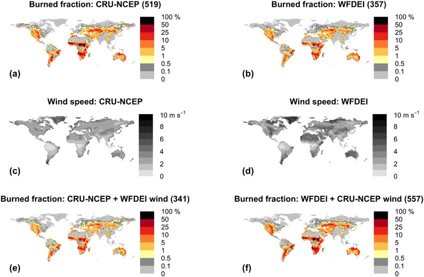
The models were spun up to a pre-industrial equilibrium
that from the WATCH data (Weedon et al., 2011), modeled
state. For these spin-up runs, population density and land
burned area decreases by ca. 27 % with important spatial
use were set to their values in 1700 CE, and atmospheric
changes in regional patterns. Because the use of different in-
CO2 concentration was set to its year 1750 CE value of
put data – in this case wind speed – can produce such major
277.33 ppm. Climate and lightning forcings from 1901–1920
differences in outputs, participating groups were allowed to
were used, being recycled until carbon values in the slowest
re-parameterize their fire models to adjust for the idiosyn-
soil carbon pool varied by less than 1 % between consecutive
crasies of the FireMIP-standardized input data.
50-year periods for every grid cell (Fig. 2). Note that for var-
Annual data from 1700 to 2013 at 0.5◦ resolution on the
ious reasons some modeling groups may not be able to use
fractional distribution of cropland, pasture, and wood har-
1700 CE as the beginning of their run, with CLM-Li prefer-
vest – as well as transitions among land-use types – were
ring 1850 and CTEM preferring 1861.
taken from the dataset developed by Hurtt et al. (2011). This
The historic simulations were run from 1700 through
dataset is based on gridded maps of cropland and pasture
2013. Population and land use were changed annually from
from version 3.1 of the History Database of the Global En-
the beginning of this simulation, and CO2 values were
vironment (HYDE; Klein Goldewijk et al., 2010), which are
changed annually from 1751 onwards. However, because the
generated based on country-level FAO statistics of agricul-
CRU-NCEP and lightning forcing data were not available for
tural area in combination with algorithms to estimate popu-
1700–1900, the 1901–1920 forcings were recycled for the
lation, land use, and settlement patterns into the past. HYDE
first 200 years of the simulation; this allowed natural climate
also provides gridded maps of historical population density,
variability to be captured while incorporating only minimal
which participating FireMIP groups used if needed.
human influence. From 1901 to 2010, time-varying values
A global, time-varying dataset of monthly cloud-to-
of all variables were used. Finally, the lightning dataset did
ground lightning was developed for this study at 0.5◦
not include 2011–2013, so the 2010 values were used for the
and monthly resolution (J. Kaplan, personal communica-
last three years of the experiment. A visualization of the time
tion, 2015), comprising global lightning strike rate (strikes
periods covered by each input in the spinup and historical
km−2 day−1 ), for the period 1871–2010. This dataset incor-
model runs can be found in Fig. 2.
porates interannual variability in lightning activity using the
Although agriculture (cropland and pasture) were speci-
method described by Pfeiffer et al. (2013) by scaling a mean
fied inputs, each model calculated natural vegetation accord-
monthly climatology of lightning activity (covering 2005–
ing to its standard set-up and no attempt was made to stan-
dardize this. The biogeography of natural vegetation, rep-
Geosci. Model Dev., 10, 1175–1197, 2017 www.geosci-model-dev.net/10/1175/2017/Table 2. List of models participating in FireMIP, including contact person’s email and key references. Also included is information relating to the configuration to be used in this phase
of FireMIP. Note that “Resolution” refers to spatial and temporal resolution of the fire model only; the associated land or vegetation may update more frequently.
Fire model Land/vegetation model Dynamic vegetation N cycle? No. PFTs No. soil layers No. litter Resolution Contact
classes
Physiology LAI, Biogeography
biomass
CLM-Li fire module (Li CLM4.5–BGC (Oleson Yes Yes Yes, but not Yes 17 15 1 ∼ 1.9◦ lat. Fang Li (lifang@mail.iap.ac.cn)
et al., 2012, 2013, 2014) et al., 2013) in FireMIP × 2.5◦ long.
(F19), half-
hourly
CTEM fire module CTEM Yes Yes Yes, but not No 9 3 1 2.8125◦ , daily Joe Melton (joe.melton@canada.ca)
(Arora and Boer, 2005; (Arora and Boer, 2005; in FireMIP
Melton and Arora, 2016) Melton and Arora,
2016)
www.geosci-model-dev.net/10/1175/2017/
Fire Including Natural LM3 Yes Yes Yes No 5 20 3 2◦ lat. Dan Ward (dsward@princeton.edu)
S. S. Rabin et al.: FireMIP phase 1 protocol
& Agricultural Lands (Shevliakova et al., × 2.5◦ long.,
model LM3-FINAL; 2009; Milly et al., half-hourly
(Rabin, 2016; Rabin 2014; Sulman et al.,
et al., 2017) 2014)
Interactive Fire and JULES (Best et al., Yes Yes Yes, but No 9 4 4 ∼ 1.2414◦ lat. Stéphane Mangeon
Emission Algorithm 2011; Clark et al., without fire ×1.875◦ long., (stephane.mangeon12@imperial.ac.uk)
for Natural Environ- 2011) feedback half-hourly
ments (JULES-
INFERNO; Mangeon
et al., 2016)
JSBACH-SPITFIRE JSBACH Yes Yes Yes, but not No 12 5 2 1.875◦ , daily Gitta Lasslop
(Lasslop et al., 2014; in FireMIP (gitta.lasslop@mpimet.mpg.de)
Hantson et al., 2015a)
LPJ-LMfire (Pfeiffer LPJ (Sitch et al., 2003) Yes Yes Yes No 9 2 (plus O- 3 0.5◦ , daily Jed Kaplan (jed.kaplan@unil.ch)
et al., 2013) horizon)
LPJ-GUESS-SIMFIRE- LPJ-GUESS (Smith Yes Yes Yes Yes 19 2 3 0.5◦ , annual Stijn Hantson (stijn.hantson@kit.edu),
BLAZE et al., 2001, 2014; Lars Nieradzik
Lindeskog et al., 2013) (lars.nieradzik@cec.lu.se)
LPJ-GUESS-GlobFIRM LPJ-GUESS (Smith Yes Yes Yes Yes 19 2 2 0.5◦ , annual Stijn Hantson (stijn.hantson@kit.edu)
et al., 2001; Lindeskog
et al., 2013; Smith
et al., 2014)
LPJ-GUESS-SPITFIRE LPJ-GUESS (Smith Yes Yes Yes No 13 2 2 0.5◦ , daily Matthew Forrest
(Lehsten et al., 2009; et al., 2001; Sitch et al., (matthew.forrest@senckenberg.de)
Thonicke et al., 2010; 2003; Ahlström et al.,
Lehsten et al., 2016) 2012)
MC-Fire MC2 (Bachelet et al., Yes Yes Yes Yes 39 Depends on to- 5 0.5◦ , monthly Dominique Bachelet
2015; Sheehan et al., tal soil depth (dominique@consbio.org)
2015)
ORCHIDEE-SPITFIRE ORCHIDEE Yes Yes Yes, but not No 13 2 2 0.5◦ , daily Chao Yue
(Yue et al., 2014, 2015) in FireMIP (chao.yue@lsce.ipsl.fr)
Geosci. Model Dev., 10, 1175–1197, 2017
11791180 S. S. Rabin et al.: FireMIP phase 1 protocol
Figure 1. Comparing the effect of different wind forcing data on burned area simulated by JSBACH-SPITFIRE (Lasslop et al., 2014) over
the years 1997–2005. (a–b) Annual burned fraction (%) modeled by JSBACH-SPITFIRE using (a) the CRU-NCEP forcing data (Wei et al.,
2014) and (b) the WATCH (WFDEI) forcing data (Weedon et al., 2011). (c–d) Mean wind speed over the simulated period from (c) the
CRU-NCEP and (d) WFDEI datasets. (e–f) Annual burned fraction (%) modeled by JSBACH-SPITFIRE with switched wind forcing: (e)
CRU-NCEP except with WFDEI wind, (f) WFDEI except with CRU-NCEP wind. Numbers in sub-figure titles give mean annual global
burned area (Mha) for each run.
Spinup 1701 1749 1750 1900 1901 2010 2011 2013
Climate Rptd. 1901– 20 Rptd. 1901– 20 Historical
CO₂ 1750 val. 1750 val. Historical
Lightning Rptd. 1901– 20 Rptd. 1901– 20 Historical 2010 val.
Pop. dens.,
1701 val. Historical
land use
Figure 2. Timelines describing how the different input datasets were used in the spinup and historical model runs. The x axis is not to scale.
“Historical”: Time series of observation-based data. “Rptd. 1901–20”: Repeated time series of values from 1901 to 1920. “YEAR val.”:
Variable held constant at value for year YEAR.
resented by plant functional types (major global vegetation total fire emissions per year from the period 1700 to 2013 are
classes; PFTs), was either prescribed by modeling groups or to be provided in ASCII format.
simulated dynamically (Table 2).
3 Participating models
2.4 Output variables
A total of 11 models are running the phase 1 FireMIP sim-
A basic set of gridded outputs (Table 3) covering the pe- ulations (Table 2). All simulate fire in “natural” ecosystems,
riod 1950–2013 is required for model comparison and eval- which are composed of a variety of PFTs representing ma-
uation. An additional set of output variables (Table A1) is jor vegetation classes around the world. Some models also
provided for diagnostic purposes. All outputs are to be pro- simulate cropland, pasture, deforestation, and peat fire (Ta-
vided in NetCDF format at the native spatial resolution of ble S3 in the Supplement). Figures 3–5 use the metaphor
the model, and at either monthly or annual temporal resolu- of a flowchart to illustrate the differences among the fire
tion (Tables 3, A1). In addition to the gridded outputs, global models in terms of structural organization and process in-
Geosci. Model Dev., 10, 1175–1197, 2017 www.geosci-model-dev.net/10/1175/2017/S. S. Rabin et al.: FireMIP phase 1 protocol 1181
Fire occurs Fire count
Prob. of fire 0 to ∞ 0 or 1
Fuel size classes
Moisture
Fuel moisture
Soil moist. RH Nesterov index
Fuel size
class distribution
Fuel
Function Thresh-
old
Suppression
Ignitions or prob.:
Explicit Implicit
human
Effect per person
Fixed Spatially-varying
Population density
Ignitions or prob.:
x C2G
frac. Efficiency
lightning
Scale
to
total
Cloud-to-ground (C2G) frac.
LPJG-SPITFIRE
ORCHIDEE
LPJ-LMfire
INFERNO
MC-FIRE
JSBACH
CLM-Li*
FINAL*
CTEM
SPITFIRE
Figure 3. Modeled processes leading to fire starts for the participating models. Beginning at the bottom, models explicitly simulate processes
that their colored line passes through, with the end result being the calculation of fire count (which in most models can be any nonnegative
number, but in MC-FIRE can only be zero or one) or probability of fire. (LPJ-GUESS-SIMFIRE-BLAZE and LPJ-GUESS-GlobFIRM are
not included here because they do not calculate fire count or probability.) Fire occurrence depends on three factors: ignitions, fuel availability,
and fuel moisture. Lightning ignition count or probability are functions of the flash rate multiplied in some models by the “cloud-to-ground
fraction” (which the input data for FireMIP already includes and is thus not calculated here; dashed box) and/or by an “Efficiency” term
describing what fraction of cloud-to-ground strikes actually serve as potential ignitions. (ORCHIDEE-SPITFIRE scales cloud-to-ground flash
rate to total flash rate, then multiplies by a coefficient representing both cloud-to-ground fraction and ignition efficiency.) Human ignition
count or probability are influenced by an “effect per person” parameter, which can either be “fixed” globally or “spatially varying.” Population
density can also contribute to “suppression.” Suppression as a function of population density can be either “explicit” (i.e., calculated by a
specific function) or “implicit” (i.e., included in the initial calculation of ignitions/probability). Fuel load affects fire occurrence either as a
simple “threshold” or by the use of some more complex “function” such as a logistic curve. Some models use several “fuel size classes,”
which can be important for both fuel loading and moisture terms.
www.geosci-model-dev.net/10/1175/2017/ Geosci. Model Dev., 10, 1175–1197, 20171182 S. S. Rabin et al.: FireMIP phase 1 protocol
Table 3. Standard output variables. See Table A1 for additional, optional output variables.
Category Name Units Dimensions Time period
Fire Fire emissions: total C kgC m−2 s−1 long. lat. PFT month 1700–2013
Fire emissions: CO2 −C kgC m−2 s−1 long. lat. month 1700–2013
Fire emissions: CO−C kgC m−2 s−1 long. lat. month 1950–2013
Burned fraction of grid cell – long. lat. PFT month 1700–2013
Fireline intensity* kW m−1 long. lat. month 1950–2013
Fuel loading kgC m−2 long. lat. month 1700–2013
Fuel combustion completeness – long. lat. month 1950–2013
Fuel moisture* – long. lat. month 1950–2013
Number of fires* count m−2 yr−1 long. lat. month 1950–2013
Fire-caused frac. tree mortality – long. lat. month 1950–2013
Fire size: Mean* m−2 long. lat. month 1950–2013
Fire size: 95th percentile* m−2 long. lat. month 1950–2013
Physical properties Total soil moisture content kg m−2 long. lat. month 1950–2013
Total runoff kg m−2 s−1 long. lat. month 1950–2013
Total evapotranspiration kg m−2 s−1 long. lat. month 1950–2013
Carbon fluxes Gross Primary Production (grid cell) kgC m−2 s−1 long. lat. month 1950–2013
Gross primary production (by PFT) kgC m−2 s−1 long. lat. PFT month 1950–2013
Autotrophic respiration kgC m−2 s−1 long. lat. month 1950–2013
Net primary production (grid cell) kgC m−2 s−1 long. lat. month 1950–2013
Net primary production (by PFT) kgC m−2 s−1 long. lat. PFT month 1950–2013
Heterotrophic respiration kgC m−2 s−1 long. lat. month 1950–2013
Net biospheric production (grid cell) kgC m−2 s−1 long. lat. month 1950–2013
Net biospheric production (by PFT) kgC m−2 s−1 long. lat. PFT month 1950–2013
Land-use change C flux: to atmosphere (as CO2 ) kgC m−2 s−1 long. lat. month 1950–2013
Land-use change C flux: to products kgC m−2 long. lat. month 1950–2013
Carbon pools Carbon in vegetation kgC m−2 long. lat. month 1700–2013
Carbon in aboveground litter kgC m−2 long. lat. month 1700–2013
Carbon in soil (incl. belowground litter) kgC m−2 long. lat. month 1700–2013
Carbon in vegetation, by PFT kgC m−2 long. lat. PFT month 1700–2013
Vegetation structure Fractional land cover of PFT – long. lat. PFT year 1700–2013
Leaf area index m2 m−2 long. lat. PFT year 1950–2013
Tree height m long. lat. PFT year 1950–2013
* If calculated by model. “Crop harvesting to atmosphere” and “grazing to atmosphere” refer to carbon that is removed from the land system, but which may be emitted over
an extended time period to represent the residence time of different pools.
clusion. Whereas LPJ-GUESS-GlobFIRM and LPJ-GUESS- Some models define constant combustion and mortality fac-
SIMFIRE-BLAZE use relatively simple empirical models tors to calculate the fraction of vegetation burned or killed
to estimate grid-cell burned area directly, the other models in a fire, whereas the rest – JSBACH-SPITFIRE, LPJ-
use a process-based structure to separately simulate fire oc- GUESS-SIMFIRE-BLAZE, LPJ-GUESS-SPITFIRE, LPJ-
currence (Fig. 3) and burned area per fire (Fig. 4). Even LMfire, MC-Fire, and ORCHIDEE-SPITFIRE – vary frac-
within the process-based models, however, a wide range tional mortality and combustion based on estimated fire in-
of complexity is evident. For example, the calculation of tensity, PFT-specific plant architecture and fire resistance,
burned area per fire (Fig. 4) can be as simple as the PFT- and other factors.
specific constants used in JULES-INFERNO, or can be so The models also differ in the order in which fire-
complex as to consider factors such as human population affected live biomass is combusted (transferred to the
density and economic status, fuel moisture and loading, atmosphere) and killed (transferred to soil and/or litter
and wind speed. Translating from burned area to effects pools; Fig. 5, Tables S12–S13). CLM-Li, LM3-FINAL,
on the ecosystem shows a similar variation in model strat- LPJ-GUESS-SPITFIRE, and ORCHIDEE-SPITFIRE com-
egy, although models tend to fall into two groups (Fig. 5). bust live biomass first, then apply fire mortality to the re-
Geosci. Model Dev., 10, 1175–1197, 2017 www.geosci-model-dev.net/10/1175/2017/S. S. Rabin et al.: FireMIP phase 1 protocol 1183
Area burned
Constant
by PFT
Rothermel
ROS
Max PFT
spread rate
Wind speed
Fuel load
Duration &/or ROS
Fuel structure
Fuel moisture
RH Soil moisture Nesterov index
Duration
Const.
or dur.
Supp.
Population density
Crop frac.
Suppression
LPJG-SIMFIRE-BLAZE
GDP
LPJG-SPITFIRE
ORCHIDEE
Glob-FIRM
LPJ-LMfire
INFERNO
MC-FIRE
JSBACH
CLM-Li*
FINAL*
CTEM
SPITFIRE
Probability 0 to ∞ 0 or 1
of fire Fire count
Figure 4. Modeled processes leading from fire starts (bottom; Fig. 3) to the calculation of burned area (top). The main processes include
suppression, duration, and rate of spread (ROS). (Some variables can contribute to more than one of these processes; dark gray overlap
areas.) “Suppression” refers to the reduction of burned area per fire. Some models apply this after the calculation of other terms (as in CLM-
Li*, LM3-FINAL, LPJ-LMfire, and LPJ-GUESS-SIMFIRE-BLAZE) or it can affect fire duration (as in CTEM and JSBACH-SPITFIRE).
Suppression can be a function of “GDP,” crop fraction (“crop frac.”), or “population density.” “Fuel structure” refers to the distribution of
fuel among different size classes. The “Rothermel” equations (Rothermel, 1972) are used by some models to determine rate of spread based
on fire intensity and other factors. The LPJ-GUESS models convert burned area to a probability of fire (dotted lines), burning individual
patches stochastically. LPJ-GUESS-GlobFIRM and LPJ-GUESS-SIMFIRE-BLAZE are denoted with white stripes to indicate that they are
using purely empirical formulas to calculate grid-cell-level burned area instead of simulating fire spread.
www.geosci-model-dev.net/10/1175/2017/ Geosci. Model Dev., 10, 1175–1197, 20171184 S. S. Rabin et al.: FireMIP phase 1 protocol
Bare ground
Combusted biomass Killed biomass
All biomass Constant
"affected" but not Tissue-spec.
combusted
PFT-specific
Fuel
load Intens-
ity
Combustion
Mortality
Tissue-/size- specific
Constant
Tissue-specific Fuel moisture
PFT-specific
INFERNO (live)
PFT- Crown Crown
vs.
spec. ground scorch
Cambial
(live)
(live)
(live)
Affected
damage
Dead biomass
Bulk litter Multiple
litter classes
(dead)
(dead)
(dead)
(dead)
(dead)
(dead)
(dead)
(dead)
(dead)
(dead)
(live)
(live)
(live)
(live)
(live)
(live)
(live)
LPJG-SIMFIRE-BLAZE
LPJG-GlobFIRM
CTEM
FINAL
CLM-Li
MC-Fire
LPJG-SPITFIRE
ORCHIDEE-SPITFIRE
JSBACH-SPITFIRE
LPJ-LMfire
SPITFIRE
Area burned
Figure 5. Modeled processes leading from burned area (bottom; Fig. 4) to fire combustion and mortality (top). We distinguish between
combusted and killed biomass based on whether it is transferred to the atmosphere or to litter/soil pools, respectively. For live biomass, the
order in which combustion and fire mortality are simulated differs among the models (Sect. 3); this is illustrated by the location at which lines
diverge and where they are reduced in size. In some models, the amount of biomass “affected” by fire depends on simulated “crown scorch”
and “cambial damage.” The fraction of biomass combusted is either a constant by vegetation type (“combustion factors”) or a “tissue-/size-
specific” function dependent on “fuel moisture,” “fuel load,” and/or fire “intensity.” The fraction of biomass killed is sometimes simply all
affected biomass that was not combusted. In other models, constant “mortality factors” for each vegetation type give the fraction of vegetation
killed in burns. LPJ-GUESS-SPITFIRE and CTEM can both then simulate the creation of “bare ground” as a result of fire death, although this
will be turned off for CTEM in this phase of FireMIP (dashed line). JULES-INFERNO (cross-hatched line) does not calculate fire mortality
and only calculates fire emissions diagnostically (i.e., material is not actually transferred from vegetation to the atmosphere).
maining non-combusted biomass. JSBACH-SPITFIRE, LPJ- to litter or soil pools (i.e., experiences mortality as defined
GUESS-GlobFIRM, LPJ-GUESS-SIMFIRE-BLAZE, LPJ- here). CTEM calculates both combustion and mortality as
LMfire, and MC-Fire, on the other hand, first “kill” biomass, fractions of pre-burn biomass.
then apply combustion to that killed fraction; the remaining A more detailed and mathematical description of the fire
non-combusted fraction of “killed” biomass is transferred models can be found in Tables S1–S28. In these, to the ex-
Geosci. Model Dev., 10, 1175–1197, 2017 www.geosci-model-dev.net/10/1175/2017/S. S. Rabin et al.: FireMIP phase 1 protocol 1185
tent possible, we have included all the equations and param- ural and human-influenced fires. The original fire parameter-
eters used by each model to calculate burned area and fire ef- ization is described in Arora and Boer (2005), with Melton
fects. Based on model descriptions available in the literature, and Arora (2016) describing recent changes and its imple-
combined with unpublished descriptions, model code, and mentation in CTEM v. 2.0. The only changes between the
extensive conversations with developers, these tables repre- version of the model used here and that described by Melton
sent the most complete description yet of the inner work- and Arora (2016) are for the vegetation biomass thresholds
ings of several fire models. Units have been standardized, for fire initiation (SL ; Table S4) and the PFT-specific frac-
variable names have been harmonized, and analogous pro- tional combustion of leaves (FC \ \
l,leaf ), stems (FCl,stem ), and
cesses have been grouped together. We have also included \
litter (FCd,litter ; see Table S16).
PFT-specific parameters and equations in Tables S17–S28;
these were prescribed by the modeling groups during the de- 3.3 JULES-INFERNO
velopment of their respective fire models either due to lim-
itations of their vegetation models or intentionally based on The Interactive Fire And Emission Algorithm For Natural
development plans and priorities. Together with Figs. 3–5, Environments (INFERNO; Mangeon et al., 2016) was devel-
the tables enable the straightforward comparison of mod- oped for the UK Met Office’s Unified Model (UM) and has
els whose published descriptions often do not adhere to the been integrated within the Joint UK Land Environment Sim-
same conventions, and will be important tools in interpreting ulator (JULES; Best et al., 2011; Clark et al., 2011). JULES-
inter-model variation in the results of the experiments de- INFERNO focuses on offering a simple, stable parameteri-
scribed in this paper. They will also prove useful for other re- zation to diagnose fire occurrence, burned area, and biomass
searchers interested in how global fire models work and how burning emissions in the context of an Earth system model.
they differ from each other. It should be noted, however, that It builds upon the fire parameterization proposed by Pechony
most of these models are under continuous development; it and Shindell (2009). It is an empirical scheme that uses vapor
should not be assumed that the descriptions given here apply pressure deficit (Goff and Gratch, 1946), precipitation, and
to anything except the model versions used for this phase of soil moisture to diagnose burned area and subsequent emis-
FireMIP. sions. Within JULES-INFERNO, humans only explicitly im-
In this section, we briefly describe each participating pact biomass burning through the number of fires. The algo-
model, including details of how the model versions used for rithm foregoes physical calculations for the rate of spread, in-
FireMIP differ from any published versions. stead assigning a vegetation-dependent average burned area:
0.6, 1.4, and 1.2 km2 for fires in trees, grasses, and shrubs,
3.1 CLM fire module respectively. Because of this specificity, no outputs for fire
counts and fireline intensity are provided. Furthermore, fire-
The fire model described by Li et al. (2012, 2013, 2014), with induced tree mortality and vegetation carbon removal have
adjusted fuel moisture parameters (Li and Lawrence, 2017), not been included. The FireMIP simulations were run on a
was used in the NCAR CLM4.5-BGC land model (Oleson relatively coarse N96 grid (192 cells longitude by 145 cells
et al., 2013) to provide outputs for FireMIP. This model in- latitude).
cludes empirical and statistical schemes for modeling burned
area of and emissions from crop fires, peat fires, and de- 3.4 JSBACH-SPITFIRE
forestation and degradation fires in tropical closed forests.
A process-based fire model of intermediate complexity sim- The SPITFIRE model (Thonicke et al., 2010) was imple-
ulates non-peat fires outside croplands and tropical closed mented in the JSBACH land surface component of the MPI
forests. CLM4.5-BGC does not output fire counts and fire Earth System Model (MPI-ESM; Giorgetta et al., 2013) to
size because the two variables are not used in the schemes for account for the effect of fire on vegetation, the carbon cycle,
crop fires, peat fires, and deforestation and degradation fires and the emissions of trace gases and aerosols into the atmo-
in tropical closed forests. Note that this fire model does not sphere. The resulting JSBACH-SPITFIRE model (Lasslop
simulate fireline intensity. In addition, CLM4.5-BGC does et al., 2014) runs on a daily time step and can be applied in
not distinguish between above-ground and below-ground lit- a coupled MPI-ESM model setup as well as an offline model
ter (Koven et al., 2013). For simplicity, this model may be forced with meteorological input data. Differences between
referred to as CLM-Li, or CLM-Li* when only referring to JSBACH-SPITFIRE and the original SPITFIRE model de-
the model for non-peat fires outside croplands and tropical scribed by Thonicke et al. (2010) include a modification of
closed forests. the effect of wind speed on fire spread rate, changes to pa-
rameters related to human ignitions and fuel drying, and a
3.2 CTEM fire module dependence of fire duration on population density (Lasslop
et al., 2014). There have been several as-yet-unpublished
The Canadian Terrestrial Ecosystem Model (CTEM v. 2.0; changes to JSBACH. The conversion factor from biomass to
Melton and Arora, 2016) represents disturbance as both nat- carbon was changed from 0.45 to 0.5 to ensure consistency
www.geosci-model-dev.net/10/1175/2017/ Geosci. Model Dev., 10, 1175–1197, 20171186 S. S. Rabin et al.: FireMIP phase 1 protocol
with emission factors. The definition of the green pool was scape fragmentation, assuming that agricultural land is not
revised to include only 1 h fuel, while previously it also in- subject to wildfire. LPJ-LMfire was used to simulate the im-
cluded sapwood. Finally, combustion completeness has been pact of humans on continental-scale landscapes during the
changed to match to that used by ORCHIDEE-SPITFIRE Last Glacial Maximum (Kaplan et al., 2016) and in late
(Yue et al., 2014), which are based on a recent collection of preindustrial time (Hopcroft et al., 2017). In contrast to LPJ-
field measurements (van Leeuwen et al., 2014). GUESS-SPITFIRE, LPJ-LMfire runs in “population mode”,
where vegetation is represented by “average individuals” as
3.5 LM3-FINAL opposed to cohorts. This necessitated some enhancements to
LPJ beyond the fire model itself, including a simplified rep-
The Fire Including Natural & Agricultural Lands model (FI- resentation of vegetation structure achieved by disaggregat-
NAL; Rabin, 2016; Rabin et al., 2017) simulates global fires ing average individuals into height classes. For the FireMIP
within the Geophysical Fluid Dynamics Laboratory Land experiments described in this paper, we used LPJ-LMfire
Model version 3 (LM3; Shevliakova et al., 2009; Milly et al., v1.0 as described in Pfeiffer et al. (2013) without modifica-
2014; Sulman et al., 2014). FINAL follows the structure tions. However, to provide a bracketing scenario of anthro-
of Li et al. (2012, 2013) closely for prediction of wild- pogenic ignitions, contrasting simulations were performed
land fires with lightning and human ignition, but does not where farmers and pastoralists either ignited fire according
have special modules for deforestation and peatland fires. to our standard preindustrial formulation, or did not ignite
Previous work (Magi et al., 2012; Rabin et al., 2015) esti- any fire at all.
mated the amount of burned area from cropland, pasture, and
non-agricultural fires based on total observed burned area 3.7 LPJ-GUESS-GlobFIRM
from the Global Fire Emissions Database version 3 includ-
ing small fires (GFED3s; Randerson et al., 2012). The non- The Lund–Potsdam–Jena General Ecosystem Simulator
agricultural burned area estimates from Rabin et al. (2015) (LPJ-GUESS) dynamic global vegetation model includes the
serve as the basis for parameter estimation in FINAL, which GlobFIRM fire model (Thonicke et al., 2001) to estimate
is accomplished using an implementation of the Levenberg– global fire disturbance. GlobFIRM simulates fire once per
Marquardt method (Rabin, 2016; Rabin et al., 2017). Crop- year if enough fuel is available, with annual fire probability
land and pasture fires are computed on a monthly basis, based based on the daily water status of the upper soil layer over
on regional climatologies of burned fraction derived from a the previous year. Fuel consumption and vegetation mortal-
statistical analysis of observed burning and land cover dis- ity then depend on fire probability and a PFT-specific fire
tributions (Rabin et al., 2015). The version of FINAL used resistance parameter. (As LPJ-GUESS-GlobFIRM estimates
here enhances rate of spread in crown fires relative to sur- burned area directly, it does not generate outputs of fire count
face fires; these are distinguished using predictions of fire- or size.) While LPJ-GUESS shares many core ecophysiolog-
line intensity and vegetation height. In addition, this version ical features with the other models in the LPJ family (Sitch
of FINAL uses fire termination conditions to determine fire et al., 2003), its distinguishing feature is that it also includes
duration; whereas fire duration was previously fixed at 1 day, detailed representations of stand-level vegetation dynamics
that is now the minimum. Lastly, parameters are optimized (Smith et al., 2001). In LPJ-GUESS, these are simulated as
separately for boreal climate zones and non-boreal climate the emergent outcome of growth and competition for light,
zones. Similarly to CLM-Li*, here LM3-FINAL* will refer space, and soil resources among annual cohorts of woody
to the fire model on non-agricultural land. plants and an herbaceous understory (Smith et al., 2001).
These processes are simulated stochastically by using mul-
3.6 LPJ-LMfire tiple “patches”, each representing random samples of each
simulated locality or grid cell and which correspond to differ-
The LPJ-LMfire model (Pfeiffer et al., 2013) is based on the ent histories of disturbance and stand development (succes-
SPITFIRE model (Thonicke et al., 2010) with a number of sion). Recently, the nitrogen cycle and N limitations on pri-
modifications to improve the simulation of fire starts, fire mary production were included in LPJ-GUESS (Smith et al.,
behavior, and fire impacts. LPJ-LMfire was specifically de- 2014), as well as land management for pastures and crop-
signed for the simulation of fire in preindustrial time, and lands (Lindeskog et al., 2013).
specifies the ways in which humans use fire based on their
subsistence livelihood, breaking populations into three cate- 3.8 LPJ-GUESS-SIMFIRE-BLAZE
gories: hunter-gatherers, pastoralists, and farmers. The model
accounts for feedbacks between human agency and biogeog- The new Blaze-Induced Land–Atmosphere Flux Estimator
raphy, in particular in the way that hunter–gatherers can in- (BLAZE; Nieradzik et al., 2017) was recently implemented
crease the carrying capacity of their environment through the into the latest version of LPJ-GUESS (Lindeskog et al., 2013;
managed application of fire, i.e., niche construction. LPJ- Smith et al., 2014). Burned area is generated once per year
LMfire also simulates passive fire suppression due to land- by the empirical fire model SIMFIRE (Knorr et al., 2014,
Geosci. Model Dev., 10, 1175–1197, 2017 www.geosci-model-dev.net/10/1175/2017/S. S. Rabin et al.: FireMIP phase 1 protocol 1187
2016) based on fire weather, fuel continuity, and human pop- to a woody product carbon pool with a 25-year residence
ulation density. This annual burned area is distributed to each time (following Lindeskog et al., 2013). In cropland and pas-
month of the year based on mean observed seasonality (cli- ture patches, tree establishment is forbidden, so only grass
matology) of burned area from GFED3 (Giglio et al., 2010). PFTs are present. Lightning ignitions occur in both cropland
Fuel consumption and tree mortality are then estimated us- and pasture, but human ignitions were forbidden in crop-
ing the BLAZE module, which computes fireline intensities lands. One further change to the model compared to previ-
from existing fuel load and fire weather parameters which ous versions is that fuel moisture was taken as the average
are translated into height-dependent survival probabilities as of the standard SPITFIRE fuel moisture (calculated per fuel
described in the Population-Order-Physiology (POP) tree de- class based on a fire danger index) and soil moisture. This
mography model (Haverd et al., 2014). Mortality functions was done to take into account the vertical moisture gradient
for different biomes are derived from the literature (Hickler through the fuel bed from the topmost fuel (whose moisture
et al., 2004; van Nieuwstadt and Sheil, 2005; Kobziar et al., will equilibrate with the air moisture) and the bottommost
2006; Bond, 2008; Dalziel and Perera, 2009). The fluxes be- fuel (which will be in contact with the soil and therefore
tween live and litter pools and the atmosphere are then com- will tend to equilibrate with soil moisture). This improved
puted accordingly. the timing and magnitude of simulated burned area in devel-
opment simulations.
3.9 LPJ-GUESS-SPITFIRE
3.10 MC-Fire
The SPITFIRE model (Thonicke et al., 2010) was originally
added to the LPJ-GUESS vegetation model (Ahlström et al., The MC-Fire module (Conklin et al., 2015; Lenihan and
2012) by Lehsten et al. (2009, 2016). This implementation Bachelet, 2015) simulates fire occurrence, area burned, and
generally followed the original SPITFIRE formulation, but fire impacts including mortality, consumption of above-
initial applications employed prescribed fire regimes and did ground biomass, and nitrogen volatilization. Mortality and
not use the full set of burned area calculations in SPITFIRE. consumption of overstory biomass are simulated as a func-
This initial version also included modifications to account for tion of fire behavior and the canopy vertical structure. Fire
the detailed representation of stand-level vegetation dynam- occurrence is simulated as a discrete event, with an ignition
ics in LPJ-GUESS. For example, because many patches are source assumed to always be present and generating at most
smaller than many individual fires, each patch burns stochas- one fire per year in a grid cell. Fire return interval varies be-
tically at each time step, with the probability of a patch burn- tween minimum and maximum values for each vegetation
ing set equal to the grid-cell burned fraction in that time type, based on fuel loading and moisture. The version of MC-
step. The version of LPJ-GUESS-SPITFIRE used here ex- Fire run here is identical to the version described by Conklin
tends the version of Lehsten et al. (2009, 2016) by incorpo- et al. (2015) and Lenihan and Bachelet (2015).
rating the complete burned area calculation from SPITFIRE
(Thonicke et al., 2010), including lightning ignitions, burned 3.11 ORCHIDEE-SPITFIRE
area, fire intensity, residence time, and trace gas emissions.
However, human ignitions have been recalibrated to match The ORCHIDEE-SPITFIRE model was developed by incor-
global burned area data, and the effect of wind speed on rate porating the SPITFIRE model (Thonicke et al., 2010) into
of spread has been modified (Lasslop et al., 2014). The rain- the land surface model ORCHIDEE. All equations as de-
green phenology follows Lehsten et al. (2009, 2016) and the scribed in Thonicke et al. (2010) were implemented, except
PFT parameterization follows Forrest et al. (2015), but some for changes to lightning ignitions and combustion complete-
important parameters for post-fire mortality and biomass of ness, as well as the addition of a fuel-dependent ignition ef-
tropical trees have been updated since those publications. ficiency term (as described in Yue et al., 2014, 2015). Com-
These are as follows: tree allometry (Feldpausch et al., 2011; bustion completeness values were updated to those in Yue
Dantas and Pausas, 2013), bark thickness (Mike Lawes, un- et al. (2014, 2015), based on data published in van Leeuwen
published data), fuel bulk density (from Hoffmann et al., et al. (2014). Regional scaling factors for burned area were
2011), and maximum crown area (increased to 300 m2 based also introduced, to adjust simulated regional burned area
on Seiler et al., 2014, but taking a more conservative value for 1997–2009 to agree with that reported in version 3 of
appropriate for a global parameterization). For details see Ta- the Global Fire Emissions Database (GFED3; Giglio et al.,
ble S22. Furthermore, a simple land-use scheme was imple- 2010). The regions used were the 14 GFED regions (van der
mented for compliance with the FireMIP protocol. A time- Werf et al., 2006). Finally, the standard FireMIP lightning
evolving fraction of patches was designated as pasture or dataset was adjusted to account for the fact that the origi-
cropland based on the HYDE land-use dataset (Klein Gold- nal model (Yue et al., 2014, 2015) was calibrated using the
ewijk et al., 2010). When natural patches were converted to LIS/OTD lightning flash rate climatology (Cecil et al., 2014,
cropland or pastures, 90 % of the aboveground carbon was http://gcmd.nasa.gov/records/GCMD_lohrmc.html). Specifi-
immediately respired to the atmosphere and 10 % was added cally, the cloud-to-ground numbers provided were scaled to
www.geosci-model-dev.net/10/1175/2017/ Geosci. Model Dev., 10, 1175–1197, 20171188 S. S. Rabin et al.: FireMIP phase 1 protocol
total (i.e., cloud-to-ground plus within-cloud) flashes, so that Following the procedure described by Kelley et al. (2013)
the mean annual global lightning flash rate during 1997–2009 will help quantify the spatial and temporal biases in mean and
was the same as that given in the LIS/OTD data. variability of a range of variables important to the Earth sys-
tem. Diagnosing the ultimate causes of those biases is prob-
lematic due to the myriad interactions between fire, vege-
tation, and the atmosphere. Only targeted experiments will
4 Model evaluation allow sufficient process isolation to provide controlled tests
of the importance of different mechanisms. The SF2 experi-
4.1 Benchmarking protocol ments, in which certain processes are fixed or disabled, rep-
resent a first step in this direction. The analysis described for
The mean and variance of global agreement between model this first phase of FireMIP will likely highlight other inter-
and observations provide basic measures of model perfor- model differences that have significant impacts on perfor-
mance. Model outputs will be compared to observations us- mance, with the purpose of serving as a jumping-off point
ing the metrics devised by Kelley et al. (2013) to quantify for further experimentation and development.
model performance for individual processes. This system The complete set of observational datasets to be used in
uses normalized mean error (NME) and normalized mean this phase of FireMIP can be found in Table 4, and a descrip-
squared error (NMSE) to evaluate geographic patterns of to- tion of the criteria for choosing datasets is given in Sect. 4.3
tal values, annual averages, and interannual variability. Spa- below.
tial performance of variables measuring relative abundance
(i.e., cases where the sum of items in each cell must be equal 4.2 Comparison to empirical relationships
to one, as in the case of vegetation cover) are evaluated us-
ing the Manhattan Metric (MM) or squared chord distance Benchmarking will establish the degree to which a model
(SCD). Kelley et al. (2013) also developed metrics to assess is able to reproduce key temporal and spatial patterns in
temporal performance – for example, comparing the timing fire regimes and drivers of fire regimes, including vegetation
and length of the simulated fire season, and the magnitude of and hydrology. However, it is important to establish that the
differentiation between seasons – with observations. These model reproduces these patterns for the right reasons rather
standardized statistics allow straightforward comparison of than because it is highly tuned. Analyses involving process
model performance with regard to variables that may have evaluation focus on assessing the realism of model behavior
differences in units of many orders of magnitude. rather than simply model response, a necessary step in estab-
Kelley et al. (2013) also introduced the idea of creating lishing confidence in the ability of a model to perform well
a kind of statistical control for putting these metric scores under substantially different conditions from the present. The
into context. The “mean model” consists of a dataset of the basis of such analyses is the identification of relationships be-
same size as the observations, where every element is re- tween key processes and potential drivers, based on analyses
placed with the observational mean. Similarly, the “random of observations using tools such as generalized linear mod-
model” is produced by bootstrap resampling of the obser- els (GLMs) to isolate meaningful relationships (e.g., Daniau
vations. These datasets allow the performance of the actual et al., 2012; Bistinas et al., 2014). Model outputs can then
models to be compared against external standards in addition be interrogated to determine whether the model reproduces
to each other for individual processes of interest. If a model these relationships (e.g., Lasslop et al., 2014; Li et al., 2014).
does not perform significantly better than one using the mean We plan to apply GLMs to both observational datasets and
or random data, its usefulness may be limited. Additionally, to the corresponding model forcing variables and model out-
as the metrics used represent normalized “distance” between puts to identify relationships between fire activity and po-
models and observations, a comparison of scores shows how tential climatic, vegetative, and socio-economic drivers. This
much closer to reality one model is than another. For exam- will allow us to analyze the sensitivity of the simulated fire
ple, a model’s score of 0.5 is exactly 33 % closer to the obser- activity to various controls, as well as to evaluate how well
vations than another of 0.75 (0.5/0.75 = 33 %). Conversely, the models recreate emergent relationships seen in observa-
the second model would need to improve by 33 % in order to tional data.
provide as good a match to observations as the first.
This benchmarking system can be used to evaluate model 4.3 Observational data
performance with regard to aspects of land and vegetation
other than fire. In addition to burned area and fire emissions, The observational database assembled for FireMIP consists
we will use observational datasets of vegetation properties of a collection of datasets selected to allow systematic eval-
and hydrology to evaluate how well the models simulate the uation of a range of model processes. The system is an up-
land–vegetation system as a whole. This is especially impor- dated and extended version of that presented by Kelley et al.
tant because burning affects a wide range of Earth system (2013). As in Kelley et al. (2013), the site-based and remotely
processes, often in a non-linear manner. sensed observational datasets were chosen to fulfill a num-
Geosci. Model Dev., 10, 1175–1197, 2017 www.geosci-model-dev.net/10/1175/2017/You can also read