The Effect of Mission Duration on LISA Science Objectives
←
→
Page content transcription
If your browser does not render page correctly, please read the page content below
Noname manuscript No.
                                               (will be inserted by the editor)

                                               The Effect of Mission Duration on LISA Science
                                               Objectives

                                               Pau Amaro Seoane · Manuel Arca
                                               Sedda · Stanislav Babak · Christopher
                                               P. L. Berry · Emanuele Berti ·
                                               Gianfranco Bertone · Diego Blas ·
                                               Tamara Bogdanović · Matteo Bonetti ·
                                               Katelyn Breivik · Richard Brito ·
                                               Robert Caldwell · Pedro R. Capelo ·
arXiv:2107.09665v2 [astro-ph.IM] 12 Jan 2022

                                               Chiara Caprini · Vitor Cardoso · Zack
                                               Carson · Hsin-Yu Chen · Alvin J. K.
                                               Chua · Irina Dvorkin · Zoltan Haiman ·
                                               Lavinia Heisenberg · Maximiliano
                                               Isi · Nikolaos Karnesis · Bradley J.
                                               Kavanagh · Tyson B. Littenberg ·
                                               Alberto Mangiagli · Paolo Marcoccia ·
                                               Andrea Maselli · Germano Nardini ·
                                               Paolo Pani · Marco Peloso · Mauro
                                               Pieroni · Angelo Ricciardone · Alberto
                                               Sesana · Nicola Tamanini · Alexandre
                                               Toubiana · Rosa Valiante · Stamatis
                                               Vretinaris · David J. Weir · Kent Yagi ·
                                               Aaron Zimmerman
                                               Received: date / Accepted: date

                                               Pau Amaro Seoane
                                               Institute of Multidisciplinary Mathematics, Universitat Politècnica de València, Spain
                                               DESY Zeuthen, Germany
                                               Institute of Applied Mathematics, Academy of Mathematics and Systems Science, CAS,
                                               Beijing, China
                                               Kavli Institute for Astronomy and Astrophysics, Beijing, China
                                               Manuel Arca Sedda
                                               Astronomisches Rechen-Institut, Zentrüm     für   Astronomie,   Universität   Heidelberg,
                                               Mönchofstr. 12-14, Heidelberg, Germany
                                               Stanislav Babak
                                               Université de Paris, CNRS, Astroparticule et Cosmologie, F-75006 Paris, France
                                               Moscow Institute of Physics and Technology, Dolgoprudny, Moscow region, Russia
                                               Christopher P. L. Berry
                                               Center for Interdisciplinary Exploration and Research in Astrophysics (CIERA), Depart-
                                               ment of Physics and Astronomy, Northwestern University, 1800 Sherman Ave, Evanston, IL
                                               60201, USA
                                               SUPA, School of Physics and Astronomy, University of Glasgow, Kelvin Building, University
2                                                                 Pau Amaro Seoane et al.

Ave, Glasgow G12 8QQ, UK
Emanuele Berti
Department of Physics and Astronomy, Johns Hopkins University, 3400 N. Charles St, Bal-
timore, Maryland 21218, USA
Gianfranco Bertone
Gravitation and Astroparticle Physics in Amsterdam (GRAPPA), and Institute for The-
oretical Physics, University of Amsterdam, Science Park 904, 1098 XH Amsterdam, The
Netherlands
Diego Blas
Theoretical Particle Physics and Cosmology Group, Department of Physics, King’s College
London, Strand, WC2R 2LS London, UK
Grup de Fı́sica Teòrica, Departament de Fı́sica,
Universitat Autònoma de Barcelona, 08193 Bellaterra, Spain
Institut de Fisica d’Altes Energies (IFAE),
The Barcelona Institute of Science and Technology, Campus UAB, 08193 Bellaterra , Spain
Tamara Bogdanović
Center for Relativistic Astrophysics and School of Physics, Georgia Institute of Technology,
Atlanta, GA 30332, USA
Matteo Bonetti
Università degli Studi di Milano-Bicocca, Piazza della Scienza 3, Milano 20126, Italy
Katelyn Breivik
Center for Computational Astrophysics, Flatiron Institute, New York, NY 10010, USA
Richard Brito
CENTRA, Departamento de Fı́sica, Instituto Superior Técnico – IST, Universidade de Lis-
boa – UL, Avenida Rovisco Pais 1, 1049 Lisboa, Portugal
Robert Caldwell
Department of Physics and Astronomy, HB6127 Wilder Lab, Dartmouth College, Hanover,
New Hampshire 03755, USA
Pedro R. Capelo
Center for Theoretical Astrophysics and Cosmology, Institute for Computational Science,
University of Zurich, Winterthurerstrasse 190, CH-8057 Zürich, Switzerland
Chara Caprini
Laboratoire Astroparticule et Cosmologie, CNRS UMR 7164, Université Paris-Diderot, 10
rue Alice Domon et Léonie Duquet, 75013 Paris, France
Vitor Cardoso
CENTRA, Departamento de Fı́sica, Instituto Superior Técnico – IST, Universidade de Lis-
boa – UL, Avenida Rovisco Pais 1, 1049 Lisboa, Portugal
Zack Carson
Department of Physics, University of Virginia, P.O. Box 400714, Charlottesville, VA 22904-
4714, USA
Hsin-Yu Chen
LIGO Laboratory, Massachusetts Institute of Technology, Cambridge, Massachusetts 02139,
USA
Alvin J. K. Chua
Theoretical Astrophysics Group, California Institute of Technology, Pasadena, CA 91125,
U.S.A.
Irina Dvorkin
Institut d’Astrophysique de Paris, Sorbonne Université & CNRS, UMR 7095, 98 bis bd
Arago, 75014 Paris, France
The Effect of Mission Duration on LISA Science Objectives                                3

Zoltan Haiman
Department of Astronomy, Columbia University, 550 W. 120th St., New York, NY, 10027,
USA
Lavinia Heisenberg
Institute for Theoretical Physics, ETH Zurich, Wolfgang-Pauli-Strasse 27, 8093, Zürich,
Switzerland
Maximiliano Isi
LIGO Laboratory, Massachusetts Institute of Technology, Cambridge, Massachusetts 02139,
USA
Nikolaos Karnesis
Department of Physics, Aristotle University of Thessaloniki, Thessaloniki 54124, Greece
APC, AstroParticule et Cosmologie, Université de Paris, CNRS, Astroparticule et Cosmolo-
gie, F-75013 Paris, France
Bradley J. Kavanagh
Instituto de Fı́sica de Cantabria (IFCA, UC-CSIC), Av. de Los Castros s/n, 39005 San-
tander, Spain
Tyson B. Littenberg
NASA Marshall Space Flight Center, Huntsville, Alabama 35811, USA
Alberto Mangiagli
Laboratoire Astroparticule et Cosmologie, CNRS UMR 7164, Université Paris-Diderot, 10
rue Alice Domon et Léonie Duquet, 75013 Paris, France
Department of Physics, University of Milano - Bicocca, Piazza della Scienza 3,I20126 Mi-
lano, Italy
National Institute of Nuclear Physics INFN, Milano - Bicocca, Piazza della Scienza 3, 20126
Milano, Italy
Paolo Marcoccia
University of Stavanger, N-4036 Stavanger, Norway
Andrea Maselli
Gran Sasso Science Institute (GSSI), I-67100 L’Aquila, Italy
INFN, Laboratori Nazionali del Gran Sasso, I-67100 Assergi, Italy
Germano Nardini
University of Stavanger, N-4036 Stavanger, Norway
Paolo Pani
Dipartimento di Fisica, “Sapienza” Università di Roma & Sezione INFN Roma1, Piazzale
Aldo Moro 5, 00185, Roma, Italy
Marco Peloso
Dipartimento di Fisica and Astronomia, Università di Padova & Sezione INFN Padova, Via
Marzolo 8, I-35131 Padova, Italy
Mauro Pieroni
Blackett Laboratory, Imperial College London, SW7 2AZ, UK
Angelo Ricciardone
1Dipartimento di Fisica e Astronomia “G. Galilei”, Universitá degli Studi di Padova, via
Marzolo 8, I-35131 Padova, Italy
Alberto Sesana
Department of Physics, University of Milano - Bicocca, Piazza della Scienza 3,I20126 Mi-
lano, Italy
Nicola Tamanini
Laboratoire des 2 Infinis - Toulouse (L2IT-IN2P3), Université de Toulouse, CNRS, UPS,
F-31062 Toulouse Cedex 9, France
4                                                                Pau Amaro Seoane et al.

Abstract The science objectives of the LISA mission have been defined under
the implicit assumption of a 4-yr continuous data stream. Based on the perfor-
mance of LISA Pathfinder, it is now expected that LISA will have a duty cycle
of ≈ 0.75, which would reduce the effective span of usable data to 3 yr. This
paper reports the results of a study by the LISA Science Group, which was
charged with assessing the additional science return of increasing the mission
lifetime. We explore various observational scenarios to assess the impact of
mission duration on the main science objectives of the mission. We find that
the science investigations most affected by mission duration concern the search
for seed black holes at cosmic dawn, as well as the study of stellar-origin black
holes and of their formation channels via multi-band and multi-messenger ob-
servations. We conclude that an extension to 6 yr of mission operations is
recommended.
Keywords General Relativity · Gravitational Waves · Black Holes

Alexandre Toubiana
Université de Paris, CNRS, Astroparticule et Cosmologie, F-75006 Paris, France
Institut d’Astrophysique de Paris, CNRS & Sorbonne Universités, UMR 7095, 98 bis bd
Arago, 75014 Paris, France
Rosa Valiante
INAF-Osservatorio Astronomico di Roma, via di Frascati 33, I-00078 Monteporzio Catone,
Italy
INFN, Sezione di Roma I, P.le Aldo Moro 2, I-00185 Roma, Italy
Stamatis Vretinaris
Department of Physics, Aristotle University of Thessaloniki, University Campus, 54124,
Thessaloniki, Greece
David J. Weir
Department of Physics and Helsinki Institute of Physics, PL 64, FI-00014 University of
Helsinki, Finland
School of Physics and Astronomy, University of Nottingham, Nottingham NG7 2RD, U.K.
Kent Yagi
Department of Physics, University of Virginia, P.O. Box 400714, Charlottesville, VA 22904-
4714, USA
Aaron Zimmerman
Center for Gravitational Physics, University of Texas at Austin, Austin, TX 78712, USA
The Effect of Mission Duration on LISA Science Objectives                      5

1 Introduction

The Laser Interferometer Space Antenna (LISA) [1]1 is a space-borne gravita-
tional wave (GW) observatory selected to be ESA’s third-large class mission,
addressing the science theme of the Gravitational Universe [2]. It consists of
three spacecraft trailing the Earth around the Sun in a triangular configura-
tion, with a mutual separation between spacecraft pairs of about 2.5 million
kilometres. The laser beams connecting the three satellites are combined via
time delay interferometry (TDI) [3] to construct an equivalent pair of two
Michelson interferometers. Thanks to its long armlength, LISA will be most
sensitive in the millihertz frequency regime, which is anticipated to be the
richest in terms of astrophysical (and possibly cosmological) GW sources, in-
cluding coalescing massive black hole binaries (MBHBs) across the Universe,
millions of binaries of compact objects within our Milky Way, and stochastic
GW backgrounds (SGWBs) produced in the early Universe (see Ref. [2,4] and
references therein).
    The science objectives (SOs) and science investigations (SIs) of the LISA
mission have been defined under the implicit assumption of a 4-yr continuous
stream of data, implying that during mission operations, the downtime of
the detector is negligible compared to the effective time of data taking. If we
define Telapsed to be the time of mission operation (from first light to final
shut down) and Tdata to be the total time of effective data taking, then one
can define a duty cycle D = Tdata /Telapsed ≤ 1. The LISA proposal assumed a
duty cycle D > 0.95 [1]. Based on the performance of LISA Pathfinder (which
started scientific operations on March 8, 2016 and took data for almost sixteen
months), it is now expected that LISA will have a duty cycle D ≈ 0.75, which,
for a 4-yr mission, reduces the effective span of usable data to 3 yr.
    As we move towards mission adoption by ESA, it is necessary to define a
mission design that will fulfill the SOs spelled out in the LISA Science Require-
ments Document (SciRD) [5]. In particular, it is of paramount importance to
consider the actual condition of data taking and processing, including a real-
istic duty cycle. In this study we answer the following questions: are the SOs
formulated assuming a 4-yr continuous data stream still achieved with a duty
cycle D = 0.75? If they are not, can we achieve them through an extension of
the mission duration with the same duty cycle D = 0.75?
    Under the assumption of a duty cycle significantly smaller than D = 1,
some confusion can arise in the definition of mission duration. Therefore, we
start by clarifying the conventions adopted in this study:
 – Telapsed denotes the nominal mission duration, i.e. the time elapsed since
   LISA is first turned on, until it is turned off for the last time. The LISA
   SciRD [5] assumed Telapsed = 4 yr.
 – Tdata denotes the actual length of the usable data stream. If we have a duty
   cycle D, then Tdata = D×Telapsed . The current best estimate is Tdata = 3 yr,
   given the estimated D = 0.75.
 1   All acronyms are defined in Table 5.
6 Pau Amaro Seoane et al.
– Tsignal is the typical lifetime of a specific signal in band. Depending on
whether this is longer or shorter than Telapsed , sources are affected by mis-
sion duration in different ways.
According to the above definitions, the LISA proposal SciRD assumed D = 1,
corresponding to Telapsed = Tdata = 4 yr.
In this paper we investigate the potential science impact of increasing the
current lifetime of the LISA mission by considering the following scenarios:
– SciRD: The SciRD configuration from the LISA proposal, i.e. Telapsed =
4 yr with D = 1.
– T4C: Continuous data for 3 yr (Telapsed = 4 yr with D = 0.75, the current
baseline);
– T5C: Continuous data for 3.75 yr (Telapsed = 5 yr with D = 0.75);
– T6C: Continuous data for 4.5 yr (Telapsed = 6 yr with D = 0.75).
The above scenarios can be thought as if there were only a single long gap in
the data lasting (1 − D) × Telapsed , occurring either before or after a continuous
stretch of data taking.
Besides these continuous-data scenarios, we will also consider scenarios
where the (1 − D) × Telapsed downtime is distributed in short-duration gaps.
Assuming that the gaps have a probability distribution R p(T ) = r exp(−rT ),
such that the expected time between gaps is hT i = dT T p(T ) = 1/r, we can
define several gapped scenarios depending on the rate r as:2
– T4G5: Data for 4 yr with gaps of length 5 days such that 25% of the data
is lost (i.e. total data stream duration 3 yr), with the time between gaps
T following a distribution with r = 1/(15 days);
– T6G5: Data for 6 yr with gaps of length 5 days such that 25% of the data
is lost (i.e. total data stream duration 4.5 yr), with the time between gaps
distributed with r = 1/(15 days);
– T4G1: Data for 4 yr with gaps of length 1 day such that 25% of the data
is lost (i.e. total data stream duration 3 yr), with the time between gaps
distributed with r = 1/(3 days);
– T6G1: Data for 6 yr with gaps of length 1 day such that 25% of the data
is lost (i.e. total data stream duration 4.5 yr), with the time between gaps
distributed with r = 1/(3 days).
Since the main scope of the study is to assess how a duty cycle D = 0.75 due
to the presence of random gaps affects LISA’s capabilities to reach its SOs,
we have primarily focused on the comparison between Cases T4G5, T4G1,
T6G5, and T6G1 and the LISA-proposal assumption of 4 yr of continuous
data (SciRD).
The paper is organized as follows. The SOs identified in the SciRD docu-
ment are divided into three main science investigation domains: astrophysics,
2 In all these scenarios the duty cycle must remain D = 0.75. This means that the average
spacing between gaps must be three times longer than the chosen gap duration Tgap . For
example if Tgap = 1 day, 1/r = 3 days, and so on.The Effect of Mission Duration on LISA Science Objectives 7
cosmology, and fundamental physics. Within astrophysics, we further sepa-
rate SOs according to the relevant GW sources, and we investigate separately
MBHBs (Sec. 2); stellar-mass compact objects, both in the Milky Way and
at cosmological distances (Sec. 3); and extreme mass-ratio inspirals (EMRIs;
Sec. 4). For cosmology, we consider separately the SOs defining LISA’s poten-
tial to perform standard sirens-based cosmography (Sec. 5) and those related
to the detection of putative SGWBs of cosmological origin (Sec. 6). In fun-
damental physics, we investigate separately LISA’s capabilities to constrain
dark matter (Sec. 7), test general relativity (Sec. 8), and explore the nature
of black holes (Sec. 9). We summarize our main findings in Sec. 10. A detailed
mapping of SOs and SIs to the sections of this paper can be found in the
summary Table 4 in Sec. 10.
We caution that our simulations are not always homogeneous across SOs.
For some signals (e.g. strictly monochromatic or stochastic), to first order,
the important quantity to be considered is Tdata , regardless of the duty cycle.
Therefore, in the absence of tools for analyzing data with gaps, we some-
times consider continuous streams of length Tdata . These details are specified
case-by-case in each section below. Moreover, when gaps are included in the
calculations, those are assumed to be lost chunks of the data stream that only
affect the source signal-to-noise ratio (SNR) calculations. In reality, gaps will
also modify the properties of the noise, which can in turn further affect detec-
tion statistics and parameter reconstruction of specific sources. More detailed
parameter estimation studies (adopting e.g., the data analysis techniques de-
veloped in Ref. [6, 7]) are beyond the scope of this paper.
2 Formation, evolution, and electromagnetic counterparts of
massive black hole mergers
In this section we consider the impact of the mission lifetime on SOs related to
the formation, evolution, and electromagnetic (EM) counterparts of MBHBs.
We first examine the effect of the mission lifetime (Telapsed ) and then focus on
the impact of gaps of different length given a duty cycle D = 0.75. Our results
will be formulated in terms of three timescales: Tsignal , Telapsed , and Tdata .
Most MBHBs stay in the LISA band for a period of time (weeks, at most
months) much shorter than LISA’s lifetime, hence Tsignal
Telapsed . This
means that the number of observed sources scales linearly with Telapsed . It
is therefore important to investigate the effect of gaps of different lengths
on the resulting number of detections and compare it to a scenario with a
continuous data stream. We thus focus on comparing the SciRD, T4G1, and
T4G5 scenarios, with the understanding that results scale linearly for longer
mission duration.
We run the light seed (hereafter popIII, since the seeds originate from
Population III stars) and heavy seed models used in Ref. [8].3 The two models
3 The heavy seed model is equivalent to the model Q3d in Sec. 5.8 Pau Amaro Seoane et al.
Fig. 1 SNR distribution for MBHBs in the popIII (left) and heavy seed (right) cases. In both
scenarios we assume Telapsed = 4 yr. We compare observational scenarios with continuous
data (SciRD) and data with gaps of different length and D = 0.75 (T4G1, T4G5), as labeled
in the figure. The legends show the number of sources observed with SNR > 8.
describe the co-evolution of MBHBs with their host galaxies assuming that
MBH progenitors are either light (∼ 100 M ; popIII remnants) or heavy
(105 M ) seeds forming at redshifts 15 < z < 20. In both models, MBHBs
are driven to coalescence via interactions with stars, gas, and/or a third black
hole, and the evolution of their orbital eccentricity is followed self-consistently
(see Ref. [8] for details).
Using these fiducial models, in which binary merger timescales (of the
order of millions to billions of years) depend on the host galaxy properties,
we first assess the impact of gaps on the overall number of detections. We
thus generate a Monte Carlo sample of 100 yr of MBHB mergers and consider
either continuous observations or data with 1 day or 5-day gaps resulting in
D = 0.75. To assess the global impact of gaps, we divide this set in 25 chunks of
4 yr each and compute the number and SNR distribution of detected systems
for the cases SciRD, T4G1, and T4G5. We assume SNR = 8 as a detection
threshold.
The results reported in Fig. 1 show that the impact of gaps depends on
the nature of MBH seeds. In the heavy seeds case, compared to the SciRD
scenario, there is no loss of detections (> 99% detections) in the T4G1 scenario,
whereas in the T4G5 scenario 95% of the systems are still detected. Gaps have
a stronger impact in the popIII case where, compared to SciRD, 88% and 85%
of the sources are still detected in the T4G1 and T4G5 scenarios, respectively.
The first thing to notice is that those fractions are always larger than the 75%
duty cycle. This is because MBHBs stay in band for weeks or more, as shown
by the SNR accumulation depicted in Fig. 2 (from Ref. [9]) for systems of
total mass 3 × 10⁵ M , 3 × 10⁶ M , and 107 M at z = 1. Random gaps of
few days will remove portions of the signal, but in the vast majority of the
cases there will still be enough SNR build-up to guarantee detection. ThisThe Effect of Mission Duration on LISA Science Objectives 9
is especially true if gaps are short and sources have high SNR, which is the
case for heavy seeds and T4G1. The longer are the gaps and the lower is the
typical source SNR, the higher are the chances that sources end up below the
detection threshold. This is why gaps are more detrimental if they last 5 days
and in the popIII scenario.
Despite introducing a duty cycle has a sub-linear effect on the overall num-
ber of detections, there are specific types of sources that might be more severely
affected, jeopardizing some of the LISA mission goals. In the following, we fo-
cus on the opposite ends of the MBHB spectrum, namely low-mass seeds at
high redshift and low-redshift massive systems. Again, we fix Telapsed = 4 yr
and compare configurations SciRD, T4G5, and T4G1.
The number of observed high-redshift (z > 10), low-mass (M < 103 M )
systems is severely impacted by the presence of gaps reducing the duty cycle
to D = 0.75. This is due to a combination of features that are unique to those
systems: they are often close to the SNR observability threshold (SNR = 8, for
MBHBs), they have Tsignal
Telapsed , but at the same time Tsignal
Tgap .
Therefore, gaps affect pretty much all of these sources and including gaps in
the data causes many of them to drop below the SNR threshold.
More specifically, in the SciRD case we expect ≈ 25 observable sources
with M < 103 M in the popIII scenario. This number drops to . 10 when we
consider configurations T4G5 and T4G1, as shown in the left panel of Fig. 3.
These results are qualitatively consistent with the findings of Ref. [10], specif-
ically their Light Seed noSN models, which are similar to the one used here,
and the unscheduled gaps scenario with 3-day gaps. For this configuration,
Ref. [10] finds that the number of observed sources is reduced by ∼ 50% rela-
tive to the case without gaps. However, Ref. [10] used a more pessimistic gap
scenario than the one considered here, which led to an effective duty cycle of
D ' 0.65, compared with D ' 0.75 in our case.
To quantify uncertainties due to model assumptions, we carry out a similar
investigation for alternative (more pessimistic) popIII seed models including
supernova feedback and other effects that dramatically reduce the number of
potential LISA sources (see Ref. [11] for details). We find that the number
of detected low-mass (M < 103 M ) systems drops from ≈ 10 in the SciRD
case to . 6 in the T4G5 and T4G1 scenarios. It is therefore clear that includ-
ing a 75% duty cycle into a four year mission operation baseline is severely
detrimental to the observation of seed black holes.
At the other end of the MBHB spectrum, several relatively massive (M >
105 M ), nearby (z < 2) sources might experience a significant SNR drop
due to gaps, as shown in the top- and bottom-right panels of Fig. 3. About
30% of these sources experience SNR drops by more than a factor of 10. This
is more severe for 5-day gaps, in which the merger–ringdown phase of loud
signals can be lost entirely. This is emphasized in Fig. 2; especially for massive
systems, the SNR is accumulated in a relatively short period at the end of
the binary’s lifetime, which can be down to few days only. If the detection
threshold is SNR = 8, then 1-day gaps should not affect the detection of any
of these systems, whereas 5-day gaps would hinder the detection of some of10 Pau Amaro Seoane et al.
104
Mtot = 3 × 10⁵M Mtot = 3 × 10⁶M Mtot = 107M
103
SNR
102
101
th
1 week
3 days
1 day
5 hourrs
s
m r
1 meorgner
th
1 week
3 days
1 day
5 hourrs
s
m r
1 meorgner
th
1 week
3 days
1 day
5 hourrs
s
merger
r
1 hou
1 hou
1 hou
10 hou
10 hou
10 hou
1 mon
Fig. 2 SNR evolution as a function of time to merger for selected MBHBs at z = 1. In
each panel we show the median and the 68% and 95% confidence regions for a sample of
104 simulated binaries with the indicated total mass and otherwise randomized parameters
(sky location, inclination, polarization, etc.). The mass ratios are randomly drawn in the
range [0.1, 1]. (Adapted from Ref. [9].)
Fig. 3 Left: Mass and redshift distribution of sources detected assuming Telapsed = 4 yr
and continuous data (Telapsed = Tdata = 4 yr, i.e. the SciRD configuration) or data with
gaps (T4G5 and T4G1 configurations), as indicated in the figure. The bottom insets show
the relative drop in the number of detections for data with gaps compared to the SciRD
configuration. Right: The top panel shows the SNR distribution of sources with M > 105 M
and z < 2 under the same assumptions made in the left-hand plot. The bottom panel
shows the distribution of SNR ratios of continuous observations vs. observations with gaps,
highlighting the presence of a long tail of sources for which gaps imply a significant loss in
SNR.
the more massive binaries with mass above ∼ 107 M . The sources in the
figure are at z = 1, and increasing the source redshift will inevitably shorten
the effective SNR accumulation timescale, exacerbating this potential issue.
In practice, this also means that, effectively, a 6-yr mission with 1-day gaps
(T6G1) is almost equivalent to a 6-yr mission with 100% duty cycle and no
gaps (i.e. Telapsed = Tdata = 6 yr), except for a reduced SNR. However, a drop
in SNR also carries a penalty, as it implies a proportional deterioration inThe Effect of Mission Duration on LISA Science Objectives 11
parameter estimation and (most importantly) sky localization, which might
have consequences when searching for EM counterparts.
We also expect that gaps will lead to selection effects in terms of certain
spin configurations. We did not quantify this bias, but we can make some qual-
itative considerations. The spin–orbit coupling in spinning black hole binaries
can delay (hasten) the onset of the plunge phase compared when the spins are
aligned (antialigned) with the orbital angular momentum, respectively. This
is often called the orbital hang-up effect [12], and it is more pronounced for
highly spinning binaries. Therefore, gaps will introduce an observational selec-
tion effect: highly spinning binaries with aligned spins will be more likely to
be detected relative to other configurations with shorter lifetimes (antialigned,
non-spinning, etc.). The highly spinning binaries with aligned spins are also
more luminous in GWs, so the two effects would presumably be compounded.
This selection effect is expected to be more severe for longer gaps.
Finally, besides considering randomly distributed gaps, which are scheduled
or happen without external input, we also propose the following scenario for
consideration. Assume a long-lived GW event has already been discovered a
month prior to a MBHB merger. Unfortunately, the SNR is too low, and the
source can not be localized on the sky, but at some point well in advance
of the merger (e.g., weeks earlier) the merger time can be predicted with
an accuracy of a day or so. Within this final day it can become possible to
localize the source, issue alerts, and enable precursor EM observations, or
observations of the merger itself. This detection can be unaffected by gaps
if LISA has the capability to adaptively reschedule gaps, when they coincide
with the final day of a merger that can be predicted sufficiently in advance.
This could significantly mitigate, or eliminate, the deleterious impact of gaps
on precursor observations.
These findings have important implications for SO2 (“Trace the origin,
growth and merger history of massive black holes across cosmic ages”), and
in particular SI2.1 (“Search for seed black holes at cosmic dawn”) and SI2.3
(“Observation of EM counterparts to unveil the astrophysical environment
around merging binaries of the LISA mission”):
– With respect to SI2.1, the loss of M < 103 M sources at z > 10 caused by
gaps is substantial. For the popIII model investigated, the detection rate of
such sources is reduced from ≈ 5 yr−1 for continuous observation streams
(Telapsed = Tdata ) to ≈ 2 yr−1 in the case of the observations with gaps
and a duty cycle of 75%. Numbers can be as low as ≈ 1 yr−1 for more
pessimistic scenarios. It is therefore clear that configurations T4G5 and
T4G1 imply a significant loss of detections compared to the SciRD LISA
baseline. The only way to mitigate the effect of gaps is by extending the
mission duration. Therefore, in order to collect a large enough sample of
such sources to ascertain the origin of seed MBHs, an extension to a 6-yr
mission requirement (i.e. cases T6G5 and T6G1) is warranted.
– With respect to SI2.3, the detection rate of M > 105 M sources at z < 2
is of the order of 2 yr−1 in the investigated models. Because of gaps, about12 Pau Amaro Seoane et al.
30% of them will suffer a significant loss of SNR compared to continuous
collection of data throughout the mission lifetime, making parameter es-
timation and, particularly, sky localization problematic. In light of these
considerations and in order to maximize the multi-messenger potential of
MBHBs, an extension to a 6-yr mission requirement is warranted.
Conversely, gaps have a minor impact on SI2.2 (“Study the growth mechanism
of MBHs before the epoch of reionization”) and SI2.4 (“Test the existence of
intermediate-mass black holes”), as they do not pose a critical risk to the
detection of the sources relevant for achieving those scientific goals.
3 Stellar-mass compact objects
In this section we will study the impact of mission duration on resolved and
unresolved stellar-mass sources (Sec. 3.1) and on the observability of stellar-
origin black holes (SOBHs) similar to those detected by the LIGO Scientific
& Virgo Collaboration (Sec. 3.2).
3.1 Stellar-mass sources
Maximizing the number of detectable binaries is important to reduce the level
of the confusion noise, which further improves the detectability and measure-
ment accuracy of extra-Galactic sources at those same frequencies. This is
true even of transients which might occur during the first years of observa-
tions, as the improved understanding of the Galactic foreground can be applied
retroactively when reanalyzing data from early in the mission.
3.1.1 Resolved Sources
Most of the resolved Galactic and extra-Galactic sources at low frequency
will be nearly monochromatic, with evolution times much greater than both
Tdata or Telapsed . Thus, gaps will not have strong effects on the majority of the
resolved Galactic sources. However, in the cases where the frequency evolution
occurs on similar timescales to the duty cycle, e.g., SOBHs (see Sec. 3.2), gaps
can reduce the fidelity of the parameter estimation of these sources.
The Galactic binary signals qualitatively scale as
1 2
h ∝ Tdata exp iπ f Telapsed + f˙Telapsed
p
+ ... . (1)
2
√
For an isolated binary the SNR scales as ∝ Tdata regardless of duty cycle
when not considering losses of data due to windowing or TDI interpolation
kernels. Therefore, longer observations are better, but the growth slows down
as the observing time increases: the number of resolved Galactic binaries will
increase much more quickly between years 1 and 2 of observing than betweenThe Effect of Mission Duration on LISA Science Objectives 13
√
Fig. 4 Left: The number of detectable UCBs scales between Tdata and Tdata due to
the combined effects of the increased SNR and frequency resolution. Right: The number of
detected binaries with measurable f˙ (used for breaking degeneracy between chirp mass and
luminosity distance, and for identifying interacting binaries) scales more dramatically with
2
elapsed time Telapsed , because it enters the GW phase as Telapsed .
years 5 to 6. However, in the confusion-dominated regime, the ability to distin-
guish resolvable binaries from the foreground depends on improved frequency
resolution, which scales as ∝ 1/Tdata . As a result, the number of detectable
binaries grows more rapidly than the simple SNR scaling predicts. √ The actual
number of detections lands somewhere in the middle between Tdata and Tdata
(see Fig. 4, left panel).
Detailed studies of the Galactic binary population, and the dynamics of
individual binaries, depend on measuring the time derivatives of the orbital
period. These time derivatives introduce stronger time dependence, but im-
portantly, it is the elapsed time that matters most. The first time derivative of
the frequency f˙ is used to distinguish between systems that are likely evolving
primarily due to GW emission vs. astrophysical interactions (e.g., mass trans-
fer [13–15]). In cases where the orbital evolution is dominated by GW emission,
f˙ can break degeneracies in the GW amplitude to determine the sources’ chirp
mass and luminosity distance. Ref. [16, 17] show that the characterization of
f˙ with mission durations of 4 and 8 yr leads to an increase from ∼ 1100 to
∼ 2800 double white dwarfs (DWDs) and 4 to 10 binary black holes (BBHs)
with measured masses.
The f˙ contribution to the GW phase scales as Telapsed
2
, thus at fixed Tdata
the science requirements for Galactic binaries benefit from lower duty cycles
(see Fig. 4, right panel). The second derivative of frequency depends even more
3
dramatically on observing time, scaling as Telapsed . The second derivative of the
orbital period encodes further details about dynamics (e.g., tidal interactions
between binaries! [18]) and gives an independent measure of chirp mass as
a consistency test in the case of assumed GR-dominated period evolution.
Systems with measurable f¨ will be comparatively rare, with O(10) sources
providing constraints to better than ∼ 20% after Telapsed ∼ 8 yr.
While a longer observing time from a longer mission duration will yield
more resolved sources, in the case where duty cycles are being considered,14 Pau Amaro Seoane et al.
maximizing Telapsed is more impactful to SI1.1 (“Elucidate the formation and
evolution of Galactic binaries by measuring their period, spatial and mass
distributions”) and SI1.2 (“Enable joint gravitational and electromagnetic ob-
servations of Galactic binaries to study the interplay between gravitational
radiation and tidal dissipation in interacting stellar systems”), than maximiz-
ing Tdata alone.
3.1.2 Unresolved foreground
The unresolved foreground confusion noise can be characterized as [19]
fknee − f
A −(f /f1 )α −7/3
Sgal = e f 1 + tanh (2)
2 f2
where f is the frequency, f1 and f2 are the break frequencies, fknee is the knee,
A is the overall amplitude, and α is a smoothing parameter.
This reduced empirical model was adopted after performing the analysis
described above in this section, on the same catalog of sources, but considering
different durations of the mission. Based on simulated LISA TDI time series
data with total observation duration of Tdata, max = 10 yr, and estimated
confusion noise for different fractions of Tdata, max , the parameters f1 and fknee
of Eq. (2) are related to the observation duration Tdata as:
log10 (f1 )= a1 log10 (Tdata ) + b1 ,
(3)
log10 (fknee )= ak log10 (Tdata ) + bk ,
where the parameters a1 , ak , b1 , and bk depend on the SNR threshold for de-
tectability of Galactic binaries. One of the most relevant characteristics of this
unresolved foreground is fknee , which roughly indicates the boundary between
−0.4
the stochastic and resolvable parts of the signal and scales as fknee ∼ Tdata ,
a rather mild function of the observation time. However, the reduction in the
stochastic foreground has an important impact on the SNR of other sources.
3.2 Stellar-origin black holes (SOBHs)
For the purpose of investigating the impact of mission duration on SOBHs, we
considered: Tdata = Telapsed = {3, 3.75, 4.5} yr of continuous data (T4C, T5C,
T6C); and Telapsed = {4, 5, 6} yr with a duty cycle D = 0.75 (T4G1/T4G5,
T6G1/T6G5).
SOBHs generally have observable signal durations such that Tsignal >
Telapsed . This makes the assessment of the impact of mission duration less
straightforward compared to, e.g., MBHBs. The signal duration Tsignal is also
much longer than the duration of typical gaps thus, to first order, gaps will
simply cause the SNR of the source to diminish by D1/2 . To simulate the im-
pact of data with gaps, we therefore artificially reduce the amplitude of the
GW signal by D1/2 , where D = 0.75; because of this, configuration T4C isThe Effect of Mission Duration on LISA Science Objectives 15
essentially equivalent to T4G1/T4G5, and configuration T6C is equivalent to
T6G1/T6G5.
To investigate the effects of changes in mission duration, a SOBH popu-
lation was simulated with a comoving merger rate density of 35 Gpc−3 yr−1 ,
with masses distributed flat in log space and a maximum mass cut for the
primary BH of M1 = 50M . We show the results of 1000 realizations of LISA
observations for two scenarios (continuous data or data with gaps) in Fig. 5.
We find that the number of SOBHs that can be identified with SNR> 8 in-
creases from an average of 10, for 3 years of continuous data to an average of
3/2
19, for 4.5 years of data. This corresponds to a N ∝ Tdata scaling. The number
of SOBHs observed by LISA depends on Tdata rather than Telapsed . In practice,
4.5 yr of continuous observations yield the same number of detections as 6 yr
of observations with 75% duty cycle, since the gap duration of both the T6G1
and T6G5 scenarios are much shorter than Tsignal . The number of potential
multiband sources observable by ground-based detectors within 10 years of
LISA observation also roughly doubles when increasing Tdata by 50% in sce-
narios T6C/T6G1/T6G5, going from ≈ 1.5 to ≈ 3, again assuming SNR> 8.
By increasing Tdata from 3 yr to 4.5 yr, the chance of a simulated Universe
realization yielding zero multiband sources with SNR> 8 (fbad , shown at the
bottom of Fig. 5) decreases from ≈ 20% to ≈ 5%.
These findings have an impact on SO4 (“Understand the astrophysics of
stellar origin black holes”), both SI4.1 (“Study the close environment of SOBHs
by enabling multi-band and multi-messenger observations at the time of coa-
lescence”) and SI4.2 (“Disentangle SOBH binary formation channels”) of the
LISA proposal. The possibility of observing extra-Galactic SOBHs with LISA
has been realized following the detection of GW150914. Early investigations
suggested that LISA might observe up to several hundreds such sources, with
few tens of them qualifying as multiband sources [20]. Subsequent downward
revisions of SOBH merger rates, together with the relaxation of the LISA high-
frequency sensitivity requirement, severely affected the expected numbers of
SOBHs, jeopardizing the achievement of SOs listed in the LISA proposal.
A 4 year mission with a 75% duty cycle (T4C, T4G1, T4G5) will observe on
average between 1 and 2 multiband sources with SNR > 8, with a 20% chance
of observing none, thus completely failing the the SI4.1 science objective. Ex-
tending the mission requirement to 6 yr (T6C, T6G1, T6G5) will result in a
rough doubling of multiband sources, reducing the risk of getting zero such
sources to ≈ 5%. Disentangling competitive SOBH formation channels based
on eccentricity measurements for science objective SI4.2 requires a sizable
number of detections. For example, based on calculations from Ref. [21], the
≈ 10 detections expected for Tdata = 3 yr (T4C, T4G1, T4G5) will not even
allow us to distinguish between the main field and cluster formation scenarios
at a 2σ level. Already with ≈ 20 observations, allowed by Tdata = 4.5 yr (T6C,
T6G1, T6G5), the discriminating power will increase to > 3σ.
The detection numbers reported above are ultimately very sensitive to the
intrinsic SOBH rate and to the maximum BH mass allowed by the pair in-
stability gap. In particular, the existence of SOBHs with M > 50M would16 Pau Amaro Seoane et al.
Fig. 5 Upper plot: average number (with standard deviation) of detected SOBHs as a
function of Tdata . All sources with SNR> 8 are shown by the cyan marks, and the multi-
band subset is shown by the dark-blue marks, as indicated in figure. Thick marks are for
continuous data (T4C, T5C, T6C) and thin marks for data with gaps and a duty cycle
of 75% (T4G1/T4G5, T6G1/T6G5). Thin marks have been slightly shifted to the left (by
3/2
0.005 dex) for readability. Black dotted lines show N ∝ Tdata for comparison. Lower plot:
fraction of SOBH realizations resulting in no multiband source detected with SNR> 8 as a
function of time. Thick and thin lines are for continuous data (T4C, T5C, T6C) and data
with gaps (T4G1/T4G5, T6G1/T6G5), respectively.
significantly increase the number of LISA detections. The SOBH landscape
will become clearer with the release of the complete catalog of LIGO–Virgo
O3 data. Given our current knowledge, extending the mission duration re-
quirement to 6 years might be crucial to achieve SO4 of the LISA proposal.
3.2.1 Detecting SOBHs from O1/O2 LIGO–Virgo catalogs
For concreteness, we consider the three loudest BBH systems in the LISA
band from the O1/O2 LIGO–Virgo catalog [22]: GW150914, GW170104 and
GW170823. For each of these three systems we find the best (for LISA) sky
position and polarization. We estimate the SNR distribution based on posterior
samples from the Gravitational Wave Open Science Center [23], assuming that
the system merges in 10 yr from the moment of observation. By considering
an observation time Tdata and a 100% duty cycle, we find the SNR valuesThe Effect of Mission Duration on LISA Science Objectives 17
summarized in Table 1. In addition, given the distribution of SNR we give the
probability (in percentage) of the source being above the detection threshold
(SNR > 8). As an example, for GW150914 optimally positioned on the sky, we
find a best SNR of 12.34 (for 6 years of observation), a mean SNR of 7.21 (based
on the parameters uncertainties inferred by the LIGO–Virgo Collaboration),
and a probability of having SNR > 8 after 6 yr of observation of ≈ 25%.
Table 1 LISA SNRs for the three loudest systems from the O1/O2 LIGO–Virgo catalog:
GW150914, GW170104 and GW170823.
Tdata =4 yr Tdata =5 yr Tdata =6 yr
max SNR max SNR max SNR
GW Event mean SNR mean SNR mean SNR
p(SNR > 8) p(SNR > 8) p(SNR > 8)
9.71 11.04 12.34
GW150914 5.68 6.46 7.21
2.27 12.21 25.50
6.26 6.83 7.62
GW170104 1.76 2.0 2.23
0.0 0.0 0.0
6.64 7.13 7.97
GW170823 1.57 1.78 2.0
0.0 0.0 0.0
We now consider how parameter estimation for the three systems above is
affected by the observation time. We vary the merger time between 7 yr and
20 yr from the start of LISA observation. Because these results are obtained
using a Fisher matrix analysis, small fluctuations due to numerical evaluation
of derivatives and inverting badly conditioned matrices are possible.
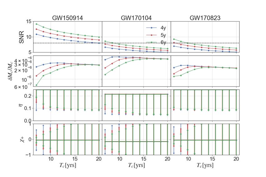
For each source, in Fig. 6 we show the SNR, the relative error on the chirp
mass Mc , and the absolute errors on the symmetric mass ratio η and on the
well-measured effective inspiral spin combination χ+ = (m1 χ1 + m2 χ2 )/(m1 +
m2 ), where χ1 is the spin aligned with the orbital angular momentum of the
primary, and χ2 is for the secondary. The chirp mass is always well determined,
while the mass ratio and spins are well determined only for systems which are
not far from merging. With 4 yr of observation we can hardly constrain the
mass ratio and spins, whereas with 6 yr of observation we can constrain the
parameters of chirping systems. The black dashed line corresponds to our
(optimistic) detection threshold SNR = 8. Because these results are obtained
assuming 100% duty cycle, a lack of data from smaller duty cycles affects the
SNR roughly as the square root of the duty cycle, so all reported errors will
increase in the same proportion.
The above results have direct impact on the detectability of GW150914-
like systems as defined by science requirement SI4.1 and on evaluation of
binary parameters for disentangling competitive SOBH formation channels
defined by science requirement SI4.2. They support the recommendation that
an extension of the mission lifetime to 6 years (T6C, T6G1, T6G5) is desirable.18 Pau Amaro Seoane et al. Fig. 6 Parameter estimation evolution as a function of the time to coalescence Tc and of the observational time. 4 Extreme- and intermediate-mass ratio inspirals: detection, characterization, population Extreme mass-ratio inspirals (EMRIs) consist of a stellar-mass compact object inspiralling into a MBH. The mass ratio is typically expected to be ∼ 10−4 – 10−6 , meaning that the system completes many orbits emitting GWs in LISA’s frequency band. Tracking the orbital evolution hence enables precision mea- surements of the system’s properties and a characterization of the spacetime of the MBH. For this reason EMRIs are important for understanding the as- trophysics of MBHs and their environments and for testing the Kerr nature of black holes. More extreme mass-ratio systems, such as those composed of a substellar-mass brown dwarf and massive black hole, are known as extremely large mass-ratio inspirals (XMRIs). These evolve even slower than EMRIS, negligibly changing over the lifetime of the LISA mission. Less extreme mass- ratio systems, such as either an intermediate-mass black hole and a MBH, or a stellar-mass compact object and an intermediate-mass black hole, are known as intermediate mass-ratio inspirals (IMRIs). These evolve quicker than EM- RIs, and are more comparable to MBHBs or SOBHBs. We concentrate here on canonical EMRIs. Changes to observing time, mission duration and gaps can effect the mea- sured SNR (Sec. 4.1), make it more difficult to track the phase (Sec. 4.3), and affect the total phase across the observations (Sec. 4.3). These effects can
The Effect of Mission Duration on LISA Science Objectives                              19

                            EMRImodel1,   gappy data
                            EMRImodel1,   continuous data
                            EMRImodel2,   gappy data
                    400     EMRImodel2,   continuous data

                    350
                N

                    300

                    250

                    200
                          3.0                 3.5                4.0   4.5
                                                    Tdata [yr]

Fig. 7 Number of EMRIs observed with SNR> 8 as a function of Tdata for two representa-
tive models from [24]. The plot shows that Tdata sets the number of detections, regardless
                                                                         3/2
of the presence of gaps, and that the number of detections is roughly ∝ Tdata .

change the number of detections and the precision to which we can perform
measurements.

4.1 Changes in SNR

EMRIs are long-lived signals that accumulate their SNR over the observable
lifetime of the inspiral. The number of detectable events increases faster than
linearly with observing time Tdata . This is because while the number of EMRIs
merging goes linearly with time, we also integrate for longer, meaning that
quieter signals can accumulate sufficient SNR to become detectable.
    The presence of gaps will decrease the SNR: to first order, the presence of
a gap is effectively equivalent to changing the mission lifetime. The final parts
of the signal are the loudest, so gaps during these times have the greatest cost.
    To support these statements, we ran representative models from Ref. [24]
with the same assumptions made for SOBHs in Sec. 3. Results are shown in
Fig. 7. Similarly to the SOBH case, the number of observations is set by Tdata ,
                                                         3/2
regardless of the presence of gaps, and we find N ∝ Tdata .
    Maximizing the potential for detection is extremely important if EMRIs
are rare. This could be the case if tightly bound low-mass objects like brown
dwarfs around MBHs are common [25,26]. These XMRI systems would not be
detectable at cosmological distances, but they could disrupt the evolution of
20 Pau Amaro Seoane et al.
EMRIs, leading to scattering of the EMRI compact object before it enters the
LISA band.
4.2 Missing phase
As EMRIs are long-lasting and slowly evolving signals, we should be able to
track the GW phase across interruptions, enabling us still to perform matched
filtering to dig the signals out of the noise. Complications arise if there is a
more sudden and distinctive change in phase during a gap.
A significant change in the phase evolution could happen if the EMRI
passes through a transient resonance. These can occur due to radiation re-
action in completely isolated systems (self-force resonance [27]), or the tidal
perturbation from a small third body (tidal resonance [28]). Transient reso-
nances are common, but only a few should have a noticeable impact [29–31].
While missing the observation of a transient resonance would mean that we
would not have the data at the time of the phase jump, this need not be a
significant problem for detection or parameter estimation.
Even though the change in phase is extremely sensitive to the orbital pa-
rameters on resonance, templates that account for resonance will still allow
coherent filtering of the pre- and post-resonance data. This could be done
in a fully modeled and self-consistent way [32, 33], or through the addition
of phenomenological resonance parameters [34]. An alternative approach is
semicoherent analysis, which could enable the phase jump to be reconstructed
without the use of resonance models.
4.3 Extra phase
Extending the mission lifetime Telapsed means that there is potentially a greater
observable phase change across the observing window. Assuming that the evo-
lution can be tracked across the entire mission (even if semicoherent methods
are used for initial detection, it may be possible to perform a coherent follow-
up analysis), we can measure the total phase evolution, tracking its change
with time even if there are gaps.
The extended baseline gives greater sensitivity to quantities which affect
the phase. This means greater measurement precision for parameters at a given
SNR, which are essential for meaningful tests of relativity and the Kerr solution
if the number of observed EMRIs is low. Measurements of environmental effects
may also benefit from this extra observation time, as the phase change can
increase superlinearly: for EMRIs in accretion disks, the scaling may be ∼
2 4
Telapsed –Telapsed [35].
Overall, since EMRIs are long-lived signals, data gaps are unlikely to cause
a significant loss in scientific performance for astrophysics, provided that wave-
forms and analysis algorithms are developed to account for gaps. However, the
presence of gaps will reduce the overall observing time, which could have anThe Effect of Mission Duration on LISA Science Objectives 21
impact on the measurement precision. Long gaps might also discard valu-
able information about transient effects such as resonances, or potential high-
frequency effects such as quasinormal bursts [36, 37]. An increase in mission
lifetime enables observation of a greater change in phase, enabling more pre-
cise measurements at a given SNR, assuming that the phase can be tracked
coherently across the entire duration.
In summary, although LISA’s SO3 (“Probe the dynamics of dense nuclear
clusters using EMRIs”) can likely be achieved by a 4-yr mission, several aspects
of EMRI observations have superlinear scaling, indicating a clear preference
for an extension of the mission lifetime requirement to 6 yr.
5 Estimation of cosmological parameters
We report here on the impact of data stream duration with and without the
presence of gaps on SI6.1 (“Measure the dimensionless Hubble parameter by
means of GW observations only”) and SI6.2 (“Constrain cosmological param-
eters through joint GW and EM observations”).
5.1 Measurement of the Hubble parameter with EMRIs
In the SciRD, SI6.1 concerns the capability of LISA to constrain the Hubble
parameter today, H0 , by using SOBHB and EMRIs as luminosity distance
indicators, together with a statistical technique to identify the redshift, based
on the cross-correlation of the GW measurement with galaxy catalogs. Prelim-
inary results using only EMRIs as distance indicators hinted to the fact that
with 4 years of continuous data it is possible to constrain the Hubble param-
eter today to about 1.7% at 1σ (cf. Fig. 8). The analysis also considers 10 yr
of continuous data, finding in that case the 1σ uncertainty ∆H0 /H0 ' 1.3%.
These results have since been confirmed by the analysis of Ref. [38], in the
context of the most optimistic scenario for the EMRIs formation.
Interpolating between
√ these two results with a scaling of the relative error
proportional to 1/ Tdata one would obtain that a 5-year mission with D =
0.75, corresponding to 3.75 yr of continuous data stream, is necessary to fulfill
SI6.1, i.e. providing a measurement of H0 to better than 2% at 1σ.
5.2 Measurement of the cosmological parameters with MBHBs
We now turn to SI6.2, which refers to the capability of LISA to constrain cos-
mological parameters using MBHB as luminosity distance indicators, together
with EM counterparts to determine the redshift.
For this analysis, we adopt the methodology developed in Ref. [39]. The
technique to identify the counterpart can be either direct observation of the
host galaxy (in particular, we modeled detection with the LSST), or connecting
the GW source with a transient occurring at the moment of the MBHB merger,22 Pau Amaro Seoane et al.
0.025
EMRIs
PRELIMINARY
H0 /H0 [68% C.L.]
0.020 0.0363738
H0 /H0 =
Tobs
data
0.015
0.010
2 4 6 8 10
Tdata
obs [yrs] (no gaps)
Fig. 8 Relative error on the Hubble parameter today, as a function of Tdata , from a pre-
liminary analysis using EMRIs as distance indicators. The blue points show the two results
obtained for 4 years of continuous data stream and 10 years √ of continuous data stream.
The purple, dashed line shows the scaling proportional to 1/ Tdata that has been used to
extrapolate the results for different data stream duration (3 yr, 3.75 yr and 4.5 yr, as shown
by the dotted grey lines.)
e.g., a radio jet. In this last case, we have implemented sky localization with
the SKA and redshift identification from the host galaxy with the ELT [39].
We analyzed three astrophysical models for the formation of the MBH, two
with high-mass seeds (Q3d, which provides the lowest number of sources, and
Q3nd, which provides the highest one) and one with low-mass seeds (popIII,
giving an intermediate number of sources) [39].
We analyzed the following duration scenarios, all with D = 0.75: continuous
data stream of 4 yr, 5 yr and 6 yr (T4C, T5C and T6C); 4 yr data stream with
1-day and 5-day gaps (T4G1, T4G5); and 6 yr data stream with 1-day and
5-day gaps (T6G1, T6G5). Figure 9 shows the distribution of standard sirens
as a function of redshift for the different duration scenarios. The majority of
standard sirens resides in the redshift range 1 < z < 3 (the more optimistic
astrophysical model Q3nd presents a significant number of sources also at
z < 1). The number of standard sirens scales linearly with the data stream
duration, and the scenario providing the highest number of standard sirens
is T6G5. In scenarios with gaps, it is less likely to completely miss a source,
while shorter and more frequent gaps lead to the highest SNR loss.
In Fig. 10 and Table 2 we present the 1σ relative uncertainties on h and
Ωm , where h = H0 /(100km s−1 Mpc−1 )) and Ωm is the relative fraction of
(dark) matter energy density today, for all 3 MBHB astrophysical formation
channels and all data stream duration scenarios, The uncertainties naturally
scale inversely to the square root of the number of standard sirens: therefore,
the best case scenario is the one with 6 yr data stream, and 5-day gaps.
We adopt as a Figure of Merit a threshold error on H0 less than 4% for
at least two formation channels. This is met by two of the duration scenarios:
6 yr data stream with 1-day and 5-day gaps, T6G1 and T6G5. The error on
H0 strongly depends on the MBHB formation channel. In the best case (Q3nd,The Effect of Mission Duration on LISA Science Objectives 23
Pre-merger(5h) - pop3 - SciRD
4
4yrs NoGaps
MBHBs with EM counterpart
5yrs NoGaps
3
6yrs NoGaps
4yrs 1dGaps
6yrs 1dGaps
2
4yrs 5dGaps
6yrs 5dGaps
1
0
0 1 2 3 4 5 6 7
z
Pre-merger(5h) - Q3d - SciRD
4
4yrs NoGaps
MBHBs with EM counterpart
5yrs NoGaps
3
6yrs NoGaps
4yrs 1dGaps
6yrs 1dGaps
2
4yrs 5dGaps
6yrs 5dGaps
1
0
0 1 2 3 4 5 6 7
z
Pre-merger(5h) - Q3nd - SciRD
4
4yrs NoGaps
MBHBs with EM counterpart
5yrs NoGaps
3
6yrs NoGaps
4yrs 1dGaps
6yrs 1dGaps
2
4yrs 5dGaps
6yrs 5dGaps
1
0
0 1 2 3 4 5 6 7
z
Fig. 9 Number of standard sirens as a function of redshift for the 7 mission duration/gaps
scenarios, from left to right in the low mass seed MBHB formation channel (popIII), and in
the two high mass seeds ones (Q3d and Q3nd).
featuring high-mass seeds with no delay in the binary formation) it is always
smaller than 3.5%, while in the worst case (PopIII, featuring low-mass seeds)
it can grow to as much as 65% for the T4C mission configuration.
As a consequence of the lack of a full parameter-estimation analysis in-
cluding merger and ringdown on the MBHB catalogs considered here [39],24 Pau Amaro Seoane et al.
0.74 LCDM 0.74 LCDM 0.74 LCDM
0.72
NoGaps (75%dc) 0.72
NoGaps (75%dc) 0.72
NoGaps (75%dc)
SciRD SciRD SciRD
0.70 pop3 0.70 Q3d 0.70 Q3nd
0.68 0.68 0.68
h
h
h
0.66 LISA Tobs : 0.66 LISA Tobs : 0.66 LISA Tobs :
4 yrs 4 yrs 4 yrs
0.64 0.64 0.64
5 yrs 5 yrs 5 yrs
0.62 6 yrs 0.62 6 yrs 0.62 6 yrs
0.20 0.25 0.30 0.35 0.40 0.45 0.20 0.25 0.30 0.35 0.40 0.45 0.20 0.25 0.30 0.35 0.40 0.45
Ωm Ωm Ωm
0.74 LCDM 0.74 LCDM 0.74 LCDM
Tobs =4yrs Tobs =4yrs Tobs =4yrs
0.72 0.72 0.72
SciRD SciRD SciRD
0.70 pop3 0.70 Q3d 0.70 Q3nd
0.68 0.68 0.68
h
h
h
0.66 Gap Scenario: 0.66 Gap Scenario: 0.66 Gap Scenario:
NoGaps NoGaps NoGaps
0.64 0.64 0.64
1dGaps 1dGaps 1dGaps
0.62 0.62 0.62
5dGaps 5dGaps 5dGaps
0.20 0.25 0.30 0.35 0.40 0.45 0.20 0.25 0.30 0.35 0.40 0.45 0.20 0.25 0.30 0.35 0.40 0.45
Ωm Ωm Ωm
0.74 LCDM 0.74 LCDM 0.74 LCDM
Tobs =6yrs Tobs =6yrs Tobs =6yrs
0.72 0.72 0.72
SciRD SciRD SciRD
0.70 pop3 0.70 Q3d 0.70 Q3nd
0.68 0.68 0.68
h
h
h
0.66 Gap Scenario: 0.66 Gap Scenario: 0.66 Gap Scenario:
NoGaps NoGaps NoGaps
0.64 0.64 0.64
1dGaps 1dGaps 1dGaps
0.62 0.62 0.62
5dGaps 5dGaps 5dGaps
0.20 0.25 0.30 0.35 0.40 0.45 0.20 0.25 0.30 0.35 0.40 0.45 0.20 0.25 0.30 0.35 0.40 0.45
Ωm Ωm Ωm
Fig. 10 Estimated 1σ ellipses of the relative uncertainties on the cosmological parameters,
h and Ωm , with 75% duty cycle. Top row: continuous data stream of 4, 5 and 6 yr; middle
row: 4 yr data stream with no gap, 1-day, and 5-day gaps; bottom row: 6 yr data stream
with no gap, 1-day, and 5-day gaps. From left to right, different columns refer to different
MBHB formation channels: popIII, Q3d, and Q3nd.
the results presented above are based on the estimation of the MBHB event
parameters performed accounting for the inspiral phase only (cut 5 hours be-
fore merger). This approach underestimates the number of available standard
sirens, and consequently also the instrument performance. On the other hand,
in the absence of catalogs produced with the SciRD sensitivity in the frequency
range 10−4 Hz < f < 0.1 Hz, we have used those produced with SciRD, but
extended down to 10−5 Hz. This might overestimate the number of detected
standard sirens, although measurements at low frequency are not expected to
strongly affect the present analysis (cf. the low-frequency study [40]).You can also read