The central dogma and cosmological horizons
←
→
Page content transcription
If your browser does not render page correctly, please read the page content below
Published for SISSA by       Springer
                                                                 Received: November 18, 2021
                                                                  Accepted: January 11, 2022
                                                                 Published: January 24, 2022

The central dogma and cosmological horizons

                                                                                               JHEP01(2022)132
Edgar Shaghoulian
 David Rittenhouse Laboratory, University of Pennsylvania,
 Philadelphia, PA 19104, U.S.A.

 E-mail: eshag@sas.upenn.edu

Abstract: The central dogma of black hole physics — which says that from the outside
a black hole can be described in terms of a quantum system with exp(Area/4GN ) states
evolving unitarily — has recently been supported by computations indicating that the
interior of the black hole is encoded in the Hawking radiation of the exterior. In this
paper, we probe whether such a dogma for cosmological horizons has any support from
similar computations. The fact that the de Sitter bifurcation surface is a minimax surface
(instead of a maximin surface) causes problems with this interpretation when trying to
import calculations analogous to the AdS case. This suggests anchoring extremal surfaces
to the horizon itself, where we formulate a two-sided extremization prescription and find
answers consistent with general expectations for a quantum theory of de Sitter space:
vanishing total entropy, an entropy of A/4GN when restricting to a single static patch,
an entropy of a subregion of the horizon which grows as the region size grows until an
island-like transition at half the horizon size when the entanglement wedge becomes the
entire static patch interior, and a de Sitter version of the Hartman-Maldacena transition.

Keywords: Gauge-Gravity Correspondence, Models of Quantum Gravity, AdS-CFT Cor-
respondence

ArXiv ePrint: 2110.13210

Open Access, c The Authors.
                                                     https://doi.org/10.1007/JHEP01(2022)132
Article funded by SCOAP3 .
Contents
1 Introduction 1
2 CFT entropy in de Sitter spacetime 3
2.1 Monotonicity of matter entropy of annulus in plane 3
2.2 Generalized entropy 5
2.3 Mapping to de Sitter 5
JHEP01(2022)132
3 Central dogma for cosmological horizons 6
3.1 dS3 8
3.2 dS4 8
3.3 Inconsistency 9
4 Anchoring on the horizon 11
4.1 Physical interpretation 13
4.2 Examples 14
4.3 Encoding the exterior with one side 17
4.4 Bulk reconstruction 18
4.5 Quantum extremal surface prescription 18
5 Discussion 19
A Extremal surfaces 20
B Observer dependence 23
C Extremal surfaces on the horizon 24
1 Introduction
The gravitational path integral has provided many powerful insights since its incarna-
tion [1]. It seems both self-consistent and supported by various microscopic calculations,
beginning with [2]. It is not universally valid, motivating the conjecture that its application
is correct if and only if the gravitational theory under consideration is holographic [3]. If
this is true, then one may hope that application of the gravitational path integral in the
cosmological context can provide clues about a holographic description.
Recently, the central dogma of black hole physics — the claim that a black hole can
be described from the outside as a unitary quantum system with exp(Area/4G) states —
–1–has been supported by computations from the gravitational path integral [4, 5], build-
ing on [6–11]. Extrapolating to the cosmological context, one might hope that the cos-
mological horizon can be described from the inside as a unitary quantum system with
exp(Area/4G) states [1].
This conjecture is on much shakier ground for multiple reasons. One reason is that
there is little microscopic support for the Gibbons-Hawking entropy of cosmological hori-
zons as coming from a Hilbert space of states (although see e.g. [12–23] for holographic
perspectives). Another reason is that the zero-point entropy, which is the piece that is
interestingly fixed by the gravitational path integral, is more mysterious in the cosmolog-
ical context. This is related to the fact that you can’t create a cosmological horizon the
JHEP01(2022)132
way you can a black hole horizon. Finally, while it’s natural that the cosmological horizon
encodes the exterior (for example, when you throw something past the cosmological hori-
zon, it grows) the way a black hole encodes the interior, that leaves open some puzzles.
First, what encodes the interior of the cosmological horizon?1 Second, projecting informa-
tion using the covariant entropy bound [27] does not seem to lead to the inflating region
being encoded on the horizon [28], at least not in a conventional way. Finally, different
observers’ exteriors can overlap, leading to redundant encoding of a nature not encountered
in AdS/CFT; it would be akin to an observer in the right exterior of the eternal black hole
being able to decode the interior without access to any of the left exterior. How is this
supposed to be reconciled?
In this paper we will focus on de Sitter spacetime and do various computations of
entanglement entropy to see if the exterior of the horizon is encoded in the interior. Do-
ing something precisely analogous to the black hole context is difficult because we don’t
naturally have an asymptotic region where gravity is weak and we have infinite volume. 2
Physically, the de Sitter horizon reabsorbs its own Hawking radiation, and we can only
collect so much of it without backreacting on the spacetime. And the typical wavelength
is of the size of the observable universe. Practically, we will nevertheless assume we can
“freeze” gravity far from the de Sitter horizon, allowing us to define regions which do not
fluctuate and whose entropy we will compute. The results do not support a picture of
the interior encoding the exterior and instead suggest anchoring extremal surfaces to the
horizon itself, which we will also explore.
Summary. We use a conformal map between de Sitter and flat spacetime to constrain
computations of entanglement entropy in de Sitter. When we freeze gravity in the interior
of a piece of the static patch (and a similar antipodal region), we will show that generalized
entropy computations in de Sitter space have a natural quantum extremal surface [7, 33],
stemming from the classical extremal surface (the bifurcation surface) [34, 35], which is a
minimum in time and a maximum in space, i.e. a minimax surface instead of a maximin
surface. This leads to violations of entanglement wedge nesting, a basic consistency prin-
1
One way to try to address this is to embed a de Sitter horizon in a spacetime with a timelike bound-
ary [17, 18, 24–26].
2
In this sense, computations of entropy at I + [29, 30], or after exiting from inflation, are more analogous
to the black hole computations. Such reasoning also motivates the introduction of a “census taker” [31, 32].
–2–ciple of any such picture. The only other extremal surface is the degenerate one which sits
right on the boundary between the frozen and unfrozen regions. This leads us to consider-
ing anchoring extremal surfaces on the horizon itself, for which we formulate a two-sided
extremization procedure inspired by a similar situation in AdS/CFT. This gives sensible
results:
• The entropy of a subregion of one horizon theory grows with twice the size of the
subregion. This threatens the bound set by a quantum system with exp(A/4G) states,
but a transition occurs at half the horizon size and we remain pegged at S = A/4G
as the region size increases. The entanglement wedge transitions from none of the
JHEP01(2022)132
interior to the entire interior at this point. These features mimic the island transition
in an eternal black hole [10, 11, 36].
• The entropy of the union of the two horizons vanishes.
• The entropy of similar cuts on each horizon has a transition like that of Hartman-
Maldacena [37], switching between a connected surface which goes through the in-
flating region and a disconnected one which sits on the two horizons. This transition
stops the entanglement from exceeding the amount allowed by a horizon theory with
exp(A/4G) states.
• Entanglement wedge nesting is satisfied.
The nature of the horizon theory — in particular, its locality properties and coupling to
gravity, how it depends on the choice of horizons, and how it responds to the dynamical
nature of the horizon — will not be addressed in this work.
Entanglement entropy in de Sitter space based on horizon-anchoring was recently dis-
cussed in [38, 39] (see also [40, 41] for previous work on anchoring to the horizon).3 Al-
though the framework in [38, 39] was not explicitly two-sided extremization the results
appear similar.
2 CFT entropy in de Sitter spacetime
In this section we will use the monotonicity of matter entropy to derive some constraints
on the CFT entropy in de Sitter spacetime by conformally mapping to the plane. An
annulus in the plane will map to an angular section θ ∈ (θi , θf ) on the spatial sphere of the
t = 0 time slice. This is the entropy we want to compute. The constraints on the annulus
entropy have been worked out in e.g. [42].
2.1 Monotonicity of matter entropy of annulus in plane
Let’s begin by considering the plane, ds2 = dρ2 + ρ2 dΩ2d−2 , and radii ρ0 < ρ1 < ρ2 < ρ3 .
The entanglement entropy for an annulus between ρ ∈ (ρi , ρj ) will be denoted S(ρi , ρj ),
3
It was also discussed by the present author at a seminar at MIT in March.
–3–while the entropy for a sphere of radius ρi will temporarily be denoted S(ρi ). Strong
subadditivity S(A) + S(B) ≥ S(A ∪ B) + S(A ∩ B) says
S(ρ0 , ρ2 ) + S(ρ1 , ρ3 ) ≥ S(ρ1 , ρ2 ) + S(ρ0 , ρ3 ) (2.1)
If we take the limit ρ3 → ∞ we get
S(ρ0 , ρ2 ) ≥ S(ρ1 , ρ2 ) + S(ρ0 ) − S(ρ1 ) , (2.2)
while if we take ρ0 → 0 we get
S(ρ1 , ρ2 ) ≤ S(ρ1 , ρ3 ) + S(ρ2 ) − S(ρ3 ) . (2.3)
JHEP01(2022)132
So far this is true for an arbitrary QFTd , but for the rest of this section we consider
a CFTd>2 . Defining the finite part of the entropy as S0 , we have S0 (ρi ) = S0 (ρj ) and
S0 (ρi , ρj ) = S0 (ρj /ρi ).4 Since all divergences cancel in these expressions, we get
S0 (ρ0 , ρ2 ) ≥ S0 (ρ1 , ρ2 ) , S0 (ρ1 , ρ2 ) ≤ S0 (ρ1 , ρ3 ) (2.4)
Defining ρj /ρi = R gives
S00 (R) ≥ 0 (2.5)
for the annulus entanglement entropy, where now the single argument refers to the ratio
of radii of the annulus. In other words, the entanglement entropy of the annular region
increases as you thicken the annulus.
We can also get a constraint on the second derivative of the entropy of the annulus.
Take ρ3 = ρ2 (1 + /R), ρ0 = ρ1 (1 − /R) with R = ρ2 /ρ1 to rewrite (2.1) as
S0 (R + 2) − 2S0 (R + ) + S0 (R) ∝ S000 (R) ≤ 0 . (2.6)
We also have that
Area(S d−2 )
S0 (R → 1) ≈ −κ , S0 (R → ∞) ≈ −2F , κ > 0. (2.7)
(R − 1)d−2
The former exression comes from approximating the thin annulus as a parallel plate ge-
ometry with plates of area Area(S d−2 )ρd−2
2 and separation ρ2 − ρ1 . The sign of κ is fixed
by the constraint S0 (R) ≥ 0. The latter expression comes from computing the entropy in
0
the complement region, which should factorize into the sum of the entropies of two spheres
of radii ρ1 and ρ2 , each of which contributes −F . In three dimensions F is related to the
F -theorem and we have F > 0. In even dimensions the quantity (including its sign) is
scheme-dependent.
Altogether, we see that the function is monotonically non-decreasing from −∞ to −2F
and remains concave throughout. In particular, the first derivative decreases from +∞ all
the way to zero, by continuity taking all values inbetween.
4
Recall that the finite part of the entropy in even dimensions is scheme-dependent due to pollution from
the logarithmic divergence; we assume a position-independent scheme so that this constant ambiguity falls
out of the derivative relations below. In particular, the finite piece does not include any terms like log ρi ,
which will make an appearance in the next subsection.
–4–2.2 Generalized entropy
In our applications we will want to consider the generalized entropy:
Area
Sgen = + SCFT . (2.8)
4G
In three and four dimensions the full entropy for an annular region is given by
(3d) 2π(ρ1 + ρ2 ) (3d) (4d) 4π(ρ21 + ρ22 ) ρ1 ρ2 (4d)
SCFT = γ + S0 , SCFT = γ − 4a log 2 + S0 . (2.9)
2
The renormalization of Newton’s constant leads to divergences that cancel against the ones
JHEP01(2022)132
in the matter entropy, and the generalized entropy is expected to be a finite quantity:
Area (3d) Area (4d)
(3d)
Sgen = + S0 , (4d)
Sgen = − 4a log(ρ1 ρ2 ) + S0 , (2.10)
4G 4G
where we now have a dimensionless ρ, normalized in terms of an arbitrary length scale. We
define Sb as
(3d) (4d)
Sb(3d) = S0 , Sb(4d) = −4a log(ρ1 ρ2 ) + S0 . (2.11)
It can heuristically be thought of as the “matter” part of the generalized entropy, although
the split into the matter piece and the gravitational piece is not meaningful, since only
the combination is finite. Sb(3d) is monotonic and concave from the relations in section 2.1,
while Sb(4d) has the anomaly term to deal with. As ρ1 → ρ2 the anomaly piece contributes
(4d)
a finite amount, so we still have Sb(4d) (R → 1) ≈ S0 (R → 1). On the other hand, due to
the anomaly, the behavior under thickening the annulus depends on whether we make ρ1
smaller or ρ2 bigger. In our applications we will be concerned with making ρ1 smaller, in
which case we have
4a
− ∂ρ1 Sb(4d) (ρ1 , ρ2 ) ≥ 0 , ∂ρ21 Sb(4d) (ρ1 , ρ2 ) = + S000 (R) . (2.12)
ρ21
So the sign of the second derivative is not fixed.
2.3 Mapping to de Sitter
Let’s say we want to compute the entropy on de Sitter spacetime,
ds2 = −dt2 + cosh2 t(dθ2 + sin2 θdΩ2d−2 ) , t ∈ (−∞, ∞), θ ∈ (0, π) (2.13)
for a belt-like region θ ∈ (θ1 , θ2 ) at t = 0. Since we are at t = 0 we can do a Euclidean
computation on the sphere ds2 = dτ 2 + cos2 τ (dθ2 + sin2 θdΩ2d−2 ) at τ = 0. In Euclidean
signature the full sphere is conformally related to the plane, as can be seen by the stereo-
graphic projection:
4dx2i 1+
Pd 2
i=1 xi
ds2 = = Ω−2 dx2i , Ω= . (2.14)
(1 + i=1 xi )
2
Pd 2 2
A natural way to interpret this stereographic projection is to have Euclidean time τ run
from the south pole to the north pole. Then the (d − 1)-spheres foliated by τ map to
–5–JHEP01(2022)132
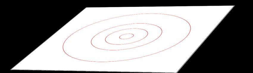
Figure 1. Two different stereographic projections. The one on the left foliates the sphere by
lower-dimensional spheres from north to south, which get projected onto the plane as spheres of
increasing radius. The one on the right foliates the sphere by lower-dimensional spheres from west
to east, which get projected onto the plane as two sets of spheres surrounding two points. The
sphere passing through the north and south poles gets mapped to a lower-dimensional plane. The
bottom line shows a direct view of the parameterization of the plane, radial coordinates on the left
and owl coordinates on the right.
(d − 1)-spheres foliated in the plane by radius. This projects the south pole to the origin
and the north pole to infinity, see the left-hand-side of figure 1.
Another interpretation is to have Euclidean time τ run from the “west” pole to the
“east” pole, while keeping the stereographic projection fixed, see the right-hand-side of
figure 1. The rest of the stereographic projection we interpret in the earlier fashion: the
(d − 2)-dimensional spheres on our τ = 0 (d − 1)-dimensional sphere map to (d − 2)-
dimensional spheres in the Euclidean plane foliated by radius. Thus, a belt like region
θ ∈ (θ1 , θ2 ) maps to an annular region ρ ∈ (ρ1 , ρ2 ) in the plane. To relate these quantities,
consider de Sitter spacetime in static patch coordinates:
dr2
ds2 = −(1 − r2 )dt2 + + r2 dΩ2d−2 = − cos2 θdt2 + dθ2 + sin2 θdΩ2d−2 (2.15)
1 − r2
In the latter coordinates, where r = sin θ, we see that θ ∈ [0, π/2] covers one static patch,
although we can continue to θ ∈ (π/2, π] to enter the neighboring static patch.
In these coordinates, a belt-like region r ∈ (r1 , r2 ) maps into an annular region
ρ ∈ (ρ1 , ρ2 ), with the relation between the two being given by the Weyl factor (or some
trigonometry)
2ρ
r= . (2.16)
1 + ρ2
3 Central dogma for cosmological horizons
Consider de Sitter spacetime again in static patch coordinates,
dr2
ds2 = −(1 − r2 )dt2 + + r2 dΩ2d−2 . (3.1)
1 − r2
–6–Pair of QM theories
=
Figure 2. The de Sitter region is replaced by a pair of quantum-mechanical theories, each described
JHEP01(2022)132
by a Hilbert space of eA/4G degrees of freedom.
This spactime has a horizon at r = 1, which has a thermodynamic entropy given by
Area(S d−2 )
S= , (3.2)
4G
similar to the thermodynamic entropy of black holes.
For the ensuing analysis we will consider an observer limited to some region r < rc ,
with rc < 1, where we freeze gravity.5 In analogy to the black hole case we will refer to
this region as the “bath” [11, 43, 44]. We will assume that the de Sitter horizon, as viewed
from the observer’s vantage point, can be thought of as a quantum system with eA/(4G)
degrees of freedom. This is represented in figure 2, where the blue curves are at r = rc . In
this exact quantum-mechanical description, we would like to compute the entropy of one
of the quantum-mechanical theories plus a small part of the bath region at time t = 0. We
will be using the QES prescription [7, 33–35], which requires extending the region into the
bulk and extremizing the generalized entropy with respect to the endpoint of the region,
see the right-hand-side of figure 3. Interestingly, we can show that there is a nontrivial
quantum extremal surface for this computation.
Before exhibiting the quantum extremal surface, let’s consider some aspects of the
classical problem. There is an obvious classical extremal surface, which is simply the
bifurcation point in the Penrose diagram. This point lies at t = 0 and therefore does not
spontaneously break the Z2 time-reflection symmetry of the problem. Notice that this
surface is quite peculiar as compared to surfaces usually considered in these problems: it
is maximal in space and minimal in time. These means that in the Euclidean computation
it will be a maximum of the action instead of a minimum. Assuming that it contributes to
the path integral, it implies that the entropy of our quantum-mechanical theory is given
precisely by A/(4G). This is simply the Gibbons-Hawking answer.
Now we consider the quantum version of the problem. First let’s remember what
happens in the case of an eternal black hole. The quantum extremal surface lives slightly
outside the horizon. This is because the area is decreasing as the horizon is approached,
5
As discussed in the introduction it is not clear that this is a sensible approximation, although the
general lesson regarding the minimax surface will apply in more reasonable spacetimes where we can freeze
gravity, e.g. embedding de Sitter in asymptotically AdS spacetime or after exiting inflation.
–7–while the matter entropy is increasing. At the bifurcation point the first derivative of the
area vanishes, so the two terms must balance somewhere before this point is reached. Thus,
the quantum extremal surface is in the right asymptotic region. For de Sitter spacetime,
as mentioned above, the area increases as the horizon is approached, which will make a
profound difference below.
We consider Einstein gravity with a positive cosmological constant coupled to CFT d .
We consider the Hartle-Hawking state for the matter on dSd . The region I˜ is a belt-like
region on the sphere S d−1 at time t = 0, with left and right endpoints given by r1 and r2 ,
respectively. By restricting to t = 0 we are assuming the Z2 time-reflection symmetry is
not spontaneously broken. The generalized entropy for this region is
JHEP01(2022)132
Area(S d−2 )r1d−2 ˜ .
Sgen = + Sbmat (I) (3.3)
4G
We now restrict to d = 3 and d = 4.
3.1 dS3
In three dimensions there is no conformal anomaly, so we have
˜ = S0 (ρ2 /ρ1 ) ,
Sbmat (I) (3.4)
where S0 (ρ2 /ρ1 ) is the finite piece of the entanglement entropy in the plane between circles
of radii ρ1 and ρ2 , as discussed in section 2. Thus the generalized entropy is
πr1
Sgen = + S0 (ρ2 /ρ1 ) , (3.5)
2G
where we can use (2.16) to go between the coordinates on the sphere and the plane. Let’s say
r2 is chosen such that there exists some rf > rc in the left static patch for which the annulus
entanglement entropy S0 (ρ2 /ρf ) factorizes into approximately −2F (see equation (2.7)).
This means there exists some r1 in the left static patch for which we have an extremum
with respect to an r1 variation, see figure 3. This is because the r1 derivative of the
gravitational entropy is positive at rf while the derivative of the matter entropy vanishes.
The derivative of the gravitational entropy approaches zero as r1 → 1, i.e. as the horizon
is approached, while the r1 derivative of the matter entropy is non-positive as it makes the
annulus thinner. This means at some point as the horizon is approached the two terms
will have equal magnitude and opposite signs. The second derivative of the gravitational
and matter entropies are both non-positive, indicating that the extremum is a maximum
in space.
By the monotonicity of the matter entropy we also know there cannot be an extremum
in the right static patch, since the sign of the derivative of the gravitational entropy flips
and matches the sign of the derivative of the matter entropy.
3.2 dS4
In four dimensions we have
˜ = S0 (ρ2 /ρ1 ) − 4a log 2ρ1 − 4a log 2ρ2 ,
Sbmat (I) (3.6)
1 + ρ21 1 + ρ22
–8–Minimax surface
x x
= x x
JHEP01(2022)132
Figure 3. The fine-grained entropy for regions specified in the exact quantum-mechanical de-
scription (left side of equality) would equal the generalized entropy for the regions specified in the
semiclassical spacetime (right side of equality) if the minimax surface shown was an acceptable
quantum extremal surface.
where the logarithmic terms have picked up a contribution from the trace anomaly, → Ω
with Ω given in (2.14). So we have
˜ = ∂ S0 (ρ2 /ρ1 ) − 4a 1 − ρ1 .
∂ b 2
Smat (I) (3.7)
∂ρ1 ∂ρ1 ρ1 + ρ31
The sign of the first term is negative by monotonicity and matches the sign of the second
term for ρ1 < 1, i.e. if we are in the left static patch. But we cannot use the same trick as
above, since starting off in the “factorized” channel where ∂ρ1 S0 (ρ2 /ρ1 ) = 0, the derivative
of the matter entropy can still have a large negative contribution from the anomaly term.
Thus it is possible that the derivative of the matter entropy is bounded above by some
negative constant −k, while the derivative of the gravitational entropy is bounded above by
O(1)/GN . If the parameters are such that k > O(1)/G then there will not be an extremum.
We can avoid these issues by making the matter entropy a small perturbation on top of
the gravitational entropy by taking a
1/G, so that a quantum extremal surface continues
to exist (its precise location will not be important to us in the following).
3.3 Inconsistency
A basic consistency check on the region defined by the quantum extremal surface is entan-
glement wedge nesting. In other words, as we move r2 to the right, we should find that r1
moves to the left. This is actually false for our putative QES above, which is related to
the fact that it is a minimax (minimum in time, maximum in space) surface instead of a
maximin surface.
Let’s consider this first in 3d. We begin with the QES at some point in the left static
patch. Moving r2 to the right decreases the first derivative of the matter entropy; it cannot
result in moving r1 to the left because this increases both the first derivative of the matter
entropy (decreasing its magnitude, since it is negative) and of the gravitational entropy,
so they can no longer cancel. Another way to think about it is to move r2 so far to the
right that the EE factorizes for r1 in the right static patch. This means the r1 derivative of
–9–the matter entropy vanishes, and will balance against the r1 derivative of the gravitational
entropy right at the bifurcation surface. In general dimension dSd>3 we can run the same
argument; in even dimensions the part of the anomaly term from ρ1 satisfies ∂ρ1 Sanom = 0
at the bifurcation surface, so we reach the same conclusion.
We can check these expectations explicitly in JT gravity in dS2 coupled to a CFT2
where we can compute the entanglement entropy analytically. The solution we will consider
is global dS obtained by an s-wave reduction of pure gravity in dS3 . We find
k
x±
1 ∼ (3.8)
x∓
2
JHEP01(2022)132
for the extremal surface, with k > 0 a semiclassical expansion parameter and x± = t ± x.
The bifurcation point is x± = 0, so x1 lives in the left static patch. We increase the size
− −
of the interval by increasing x+ 2 and decreasing x2 . This leads to x1 increasing and x1
+
decreasing, i.e. the QES also moves to the right.
A related problem with the QES reaching into the neighboring static patch is that
the purported island region of the right system will overlap with the island region of the
left system. These issues are also related to the fact that perturbations make the dS
Penrose diagram grow taller [45, 46]. At a minimum this means these two systems should
be thought of as interacting. Even interacting holographic systems, however, should obey
entanglement wedge nesting, which is violated in this setup.
The root of these various problems seems to be the inclusion of minimax surfaces in
our entanglement entropy prescription. In the context of AdS/CFT, the surfaces which
compute entanglement entropy and give reasonable behavior are always maximin surfaces.
In particular, assuming the quantum focusing conjecture, entanglement wedge nesting, and
strong subadditivity imply that the extremal surface is maximal in time [30], so it is not
a surprise that entanglement wedge nesting is violated for our minimax surface. 6 Surfaces
which are maximal in space have instead recently been interpreted as being related to
restricted complexity [49]. That is one possible role of the de Sitter bifurcation surface,
although the covariantization of maximal surfaces would have to be generalized to include
miniminimax surfaces analogous to the maximinimax surfaces of [49].7
If we exclude this surface, then the only remaining possible surface is the degenerate
one which sits right at rc as in figure 4. It is degenerate in the sense that if we minimize then
the surface runs to the boundary and can’t go any further due to the boundary conditions
6
Other arguments showing that the quantum focusing conjecture implies entanglement wedge nesting
assume asymptotically AdS boundary conditions or a maximin prescription as the definition of the extremal
surface (or both) [47, 48], so our result does not imply any problem for quantum focusing.
7
The maximinimax prescription of [49] is that on every Cauchy slice you perform a minimax procedure,
which is to sweep through all spatial slicings of the Cauchy slice, for each spatial slicing find the maximal
area surface, and then minimize this over all spatial slicings. Finally, you maximize this over all Cauchy
slices. The minimax part of the procedure is inspired by complexity in tensor networks. The maximization
in time is not something coming from tensor networks but instead provides a covariantization which gives
a nontrivial surface in e.g. the case of evaporating black holes, where a minimization would run into the
singularity. Depending on how one sets up the problem in de Sitter spacetime, both miniminimax surfaces
and maximinimax surfaces can give nontrivial answers.
– 10 –QES
x x
= x x
JHEP01(2022)132
Figure 4. The QES is given as the degenerate surface which sits right on the cutoff surface.
on the problem. In our problem rc was somewhat arbitrary, so the value implied for the
entropy inherits this ambiguity. In some sense, this is the right answer, but it is not very
useful. A natural rc to pick is the horizon, in which case the degenerate minimal surface
ends up landing on the horizon itself, giving S = A/4G, a satisfying answer. Motivated by
this, we will consider a slightly different prescription in the next section, where we anchor
extremal surfaces to the horizon itself and consider a two-sided extremization.
4 Anchoring on the horizon
Placing a holographic dual to de Sitter space on the horizon itself has a long prece-
dent [13, 28, 40, 56–58].8 There are serious questions about such a construction which
we will not address, foremost being the dynamical nature of the horizon and the properties
of the theory on the horizon: gravity does not obviously decouple there, so it seems the
holographic dual would itself be gravitational, as in [13]. In the rest of this work we will
compute entanglement entropy for cuts of the horizon as if it were a (possibly nonlocal)
quantum system. In computing entanglement entropy, however, we are faced with another
issue, which is that there is spacetime to both sides of the horizon. A similar issue has been
explored in AdS/CFT, using Karch-Randall branes [67, 68] in what has been coined “wedge
holography” [55, 69–72]. In the context of wedge holography, one has a (d − 1)-dimensional
CFT which is dual to a “wedge” in AdSd+1 bounded by two gravitating branes. However,
another description is that the (d − 1)-dimensional CFT is dual to two d−dimensional
CFTs coupled to gravity. See figure 5. These two systems are on either side of the (d − 1)-
dimensional CFT. The prescription for computing entanglement entropy for a subregion A
of the (d − 1)-dimensional CFT is to find all (d − 1)-dimensional extremal surfaces in the
(d + 1)-dimensional wedge whose boundary contains ∂A, which is (d − 3)-dimensional. The
boundaries of these extremal surfaces are (d − 2)-dimensional so will also sit somewhere on
the branes. Their location on the branes also needs to be an extremum. The entanglement
entropy is computed by the area of the minimal such surface.
8
The other natural place is I + /I − [59–62]; see [63] for a review of various approaches and e.g. [64–66]
for anchoring extremal surfaces to these boundaries.
– 11 –JHEP01(2022)132
Figure 5. We represent wedge holography as a series of modifications to the familiar example of
the top line [5, 36, 50–52]. On the top left we have the spacetime for the eternal black hole in AdS d
coupled to two flat space baths. There is a holographic CFTd everywhere in the spacetime. The top
middle represents the microscopic description, where we have a holographic CFT d−1 (represented
by a red dot) coupled to a d-dimensional bath hosting the holographic CFTd , and this joint system’s
thermofield double partner. The top right illustrates the emergent (d + 1)-dimensional description
(the thermofield double part is not represented for simplicity). In the middle line we have the
same representations, except we now have a finite bath and an additional holographic CFT d−1
(represented by a blue dot) which is also coupled to the bath CFTd (and their thermofield double
partners) [53, 54]. The Penrose diagram is identified at the left and right. The final line shrinks the
bath size to zero, so the interacting CFT’s sit right on top of one another [4, 55]. Notice in this case
the boundary dual has spacetime to both sides. In our de Sitter analogy this will be the primary
feature we are interested in, as our “boundary dual” is on the cosmic horizon and has spacetime to
both sides. The analog of the doubly emergent AdSd+1 will not play a role.
If we think only of the duality between the CFTd−1 and the two d-dimensional bulks,
this extremization can be thought of as a “two-sided” extremization which occurs on both
sides of the CFTd−1 . We no longer have a (d + 1)-dimensional bulk and a minimal surface
there, but we can understand what was being captured by that surface. Heuristically, its
boundary on the gravitating d-branes captures the d-dimensional gravitational entropy,
while its bulk piece captures the matter entropy of the theory on the d-branes (recall again
that this division is ambiguous and only the combination is expected to be finite in the
ultraviolet theory). Thus, we can dispense with this surface and simply extremize the
generalized entropy on the d-branes.
To compute extremal surfaces in global de Sitter, we therefore have the following
minimization problem. We pick a region on the union of the two horizons. We perform
a simultaneous “two-sided” extremization on both horizons with the boundary condition
defined by the chosen region. The full entanglement wedge is the region whose boundary
– 12 –JHEP01(2022)132
Figure 6. A global time slice of de Sitter, with the horizons HL and HR . The entropy of a
subregion h on HL ∪ HR is computed by an extremal surface which contains ∂h and whose interior
includes h and no other piece of HL ∪ HR . This is equivalent to breaking up the sphere into three
pieces as in the right image, and doing a single extremization where each surface is anchored to
∂h as in ordinary AdS/CFT. Thinking of the horizons as AdS boundaries makes the homology
rule identical to that case. In the classical case with topology fixed as above we can perform three
independent extremizations for each region.
is the union of the extremal surfaces found by the procedure above, and which contains
the pieces of the horizon whose entropy we are computing. In the classical case with fixed
sphere topology, this can be broken up into three independent extremizations: one for each
of the two static patch interiors, and one between the two horizons. We will allow our
extremal surfaces to have kinks across the horizons. See figure 6. (For a distinct proposal
for dealing with the other side of the horizon, see [73].)
4.1 Physical interpretation
In wedge holography, the CFTd−1 can be thought of as two CFTd−1 systems interacting
through a shared d-dimensional bath region, in the limit that the bath region shrinks to zero
size, see figure 5. We will think of our theory on the de Sitter horizon in a similar way, as
two interacting theories (not necessarily CFTd−1 ’s), one nominally describing the interior
of the horizon (we will call this the interior theory) and the other nominally describing the
exterior (we will call this the exterior theory). The word “nominally” is used here because
determining which theory describes which region of the spacetime is a dynamical question
that needs to be answered by computing entanglement wedges, and in any case the two
theories here are interacting. The interior and exterior theories are jointly in a mixed state,
purified by the partner theories on the other horizon. The exterior theories are connected
“through the bulk”, so it is like they are in a deconfined state. The interior theories are
not connected through the bulk (for empty de Sitter), so it is like they are in a confined
state. The spatial sphere caps off in the interior and does not cap off in the exterior. In
the AdS/CFT analogy we can modify the bottom row of figure 5 so that one of the two
interacting thermofield double pairs is below its Hawking-Page transition and therefore
dual to two independent thermal AdS geometries. This way the geometry caps off at either
end, like in the case of de Sitter. Alternatively, the interior theories in the case of de Sitter
can (temporarily) deconfine, as represented by the Schwarzschild-de Sitter solution, which
– 13 –has a wormhole going from one interior to the other one. This is more like the bottom
row of figure 5. These horizon theories need not have any spatial locality, so the cuts of
the horizon on which we will be anchoring our extremal surfaces need not correspond to
spatial divisions of the system. In fact, in the next subsection we will see a “volume law”
for the growth of entropy of a cut on the horizon, indicative of nonlocal behavior.
The exterior cuts across many horizons, while the interior contains just one horizon
— in the AdS/CFT analogy this would mean the exterior should be described by field
theory degrees of freedom while the interior should be described by the matrix degrees of
freedom. Studies of the entanglement properties of such matrix degrees of freedom can be
found in [69, 74–76]; our interior extremization is akin to the prescription in these papers.
JHEP01(2022)132
4.2 Examples
Let us pick a few cases to apply our proposal. We will begin by only computing classical
extremal surfaces in pure de Sitter spacetime, without any corrections from matter. In this
case the extremization problem discussed above can be broken up into three pieces: an
extremization that occurs in the interior of each static patch, and an extremization that
occurs between the two horizons.
Both horizons: S(HL ∪ HR ) = 0. If we pick the entire boundary region, i.e. both
horizons, then the extremization gives the trivial surface. To see it break up into three
pieces we have the following: if we extremize a surface homologous to either horizon and
contained in its interior, we see that it can shrink and slip off, giving the trivial surface.
Similarly, between the two horizons, the two surfaces can coalesce and again give the trivial
surface. We get S = 0 and the entanglement wedge is the entire spacetime.
One horizon: S(HL ) = S(HR ) = A/4G. If we pick one of the two horizons, then
the extremization gives the horizon we chose, with the entanglement wedge being its inte-
rior. Let’s see this from the three independent extremizations. Extremizing to the chosen
horizon’s interior gives the trivial surface with the entanglement wedge being the entire
interior, while the extremization between horizons gives the degenerate surface which sits
exactly on the chosen horizon, thus encoding none of the exterior. (There is a degenerate
surface which corresponds to the other horizon, but in such cases we are instructed to pick
the surface with the smaller entanglement wedge.) Since no region was chosen on the other
horizon no extremization is required to its interior; the entanglement wedge there is trivial.
The fact that altogether we encode only one static patch is sensible since — like with black
holes — having access to only one side restricts the reconstructible region to lay within
the corresponding horizon. (We will assume in this section that the horizons are of equal
size; see section 4.3 for a discussion of the situation where they are unequal.) An allowed
possibility which does not occur is that the chosen horizon’s interior extremization leads
to an extremal surface in the interior of the partner horizon, with the entanglement wedge
being everything to the interior of this extremal surface and everything within the original
horizon.
– 14 –S(h)
size(h)
Figure 7. Left: there are two extremal surfaces for the entropy of a subregion h of one horizon,
JHEP01(2022)132
marked as red and blue above. The minimal one exhibits a transition: the entropy of a subregion
grows as twice its size (solid red curve) until the halfway point, where it saturates at the horizon
area (solid blue curve) and the entanglement wedge becomes the interior of the horizon. This
transition will be smoothened out by anchoring at the stretched horizon. Right: the red saddle
and blue saddle drawn for configurations where they are minimal, with the entanglement wedge
shaded. (These extremal surfaces do not live at fixed global time — they are drawn that way above
for simplicity, see appendix C for a discussion.) This is reminiscent of the island transition in an
eternal black hole.
Subregion on one horizon: S(h ⊂ HL ). Subregions on the horizon are a little more
subtle. Say we choose a subregion on just one of the horizons. There are two extremal
surfaces, one with area equal to the area of the surface itself and one with area equal to
the area of the surface’s complement (restricted to the horizon).9 The smaller of the two
is clearly the minimal one for the interior extremization.
This is not quite true for the exterior extremization due to the homology constraint;
the appropriate extremal surface will always live on the horizon and have area equal to
the area of the region we are considering. The surface with area equal to the area of
the complement of our region on the horizon violates the homology constraint since the
entanglement wedge will have the partner horizon as a boundary. This leads to the following
intriguing situation. For a subset of the horizon h which is smaller than half, none of the
bulk interior or exterior is encoded, and S = 2 Area(h). This is a “volume law” growth of
the entropy, indicative of nonlocality of the dual theory. This threatens to violate unitarity
when h is half the system size and S = A/4G for A the total horizon area, but at this
point there is a transition. The exterior extremization continues to give Area(h) while the
interior extremization flips to Area(h̄). The entanglement wedge is now the entire interior
(to see this we can regulate the horizon into the stretched horizon and anchor our surfaces
there), and the entropy stays pegged at S = A/4G. This transition at half the system size
and the subsequent encoding of the interior seems tantalizingly like the island transition,
see figure 7.
We can smoothen this transition by putting our anchoring surface at the stretched
horizon. This breaks the degeneracy and for an interior extremization of a subregion on
9
These extremal surfaces do not live at fixed global time even though they will be drawn as if they do
for simplicity, see appendix C for a discussion.
– 15 –JHEP01(2022)132
Figure 8. The extremal surfaces which connect a piece of one horizon to the same piece of the
other horizon. They cease to exist past σ = π/4, before which a transition to the disconnected
surface which sits on the two horizons occurs; this is like the Hartman-Maldacena transition in
AdS/CFT. The area of this saddle diverges as σ → π/4 for all dSd>3 . For dS3 if we pick the same
interval on each horizon the length of this saddle approaches a single horizon length 2π.
the horizon produces entanglement wedges of increasingly bigger size as the subregion size
is increased.
Subregions on both horizons and a Hartman-Maldacena transition: S(hL ∪ hR ).
We can also consider similar subregions on each horizon.10 The interior extremizations
remain the same as we discussed above, although now we have a competition between
three saddles for the exterior extremization. The first two saddles are disconnected and
live on the horizon, with area equal to the area of the region we are considering or its
complement (restricted to the horizon). Any time the regions on the two horizons have
a summed area A > AdS , then the outer extremization picks the complements on the
horizon, with area 2AdS − A < AdS . In this case the entanglement wedge is the entire
inflating region, otherwise it is none of the inflating region. The third saddle is connected
across the inflating region, represented in figure 8. At early times the connected saddle
will dominate, due to the short distance between the two horizons. The entropy implied by
this saddle grows without bound for dSd>3 , threatening the bound set by finite quantum
systems with exp(A/4G) states. A transition to the disconnected saddle occurs before any
violation, and the entropy becomes time-independent. This is a de Sitter version of the
Hartman-Maldacena transition [37]. Computational details can be found in appendix A.
Notice that the exterior extremization is necessary not only to answer the question of
how the inflating region is encoded, but also to get S = A/4G in the limit where we take
one entire horizon as in the above example.
Necessity of joint extremization. The example of de Sitter-Schwarzschild simply il-
lustrates why our proposed extremization does not generically break up into separate ex-
tremizations. In particular, the two static patch interiors are now connected by a wormhole.
As usual, if we compute the full entropy, i.e. that of both cosmological horizons, we expect
to get S = 0. If we performed the interior extremizations independently then each extrem-
10
This calculation was suggested by Leonard Susskind.
– 16 –ization would land on the black hole horizon and give S = ABH /4 for ABH the area of
the black hole. Performing a joint extremization shows that the extremal surfaces can go
through the black hole wormhole and coalesce, giving S = 0 and an entanglement wedge
which covers the entire spacetime. So we see that connections between regions, either
through classical bridges or quantum entanglement (this will be introduced in section 4.5),
necessitates a joint extremization.
If we compute the entropy of one of the two cosmological horizons, we find S =
ABH /4 + ACH /4, where ACH is the area of the cosmological horizon.
As in the pure de Sitter case, the exterior extremizations for symmetric regions hL ∪hR
in this case have connected surfaces which cut across the inflating region, as long as we
JHEP01(2022)132
are not at late times. The interior extremization for Schwarzschild-de Sitter can also have
connected surfaces which cut across the black hole interior, analogous to the Hartman-
Maldacena surface for eternal black holes in AdS/CFT. In certain regimes — for example
big black holes close to the Nariai bound at early times — the dominant surface will cut
across the inflating de Sitter region and the crunching black hole region.
The quantum-mechanical problem will have to deal with the instability of de Sitter-
Schwarzschild black holes, which will greatly change the nature of the problem.
4.3 Encoding the exterior with one side
Most of the solutions we consider in dS, if starting from one static patch and analytically
extended, lead to equal-size horizons. For example if you put a particle in one static patch
to make the horizon smaller, the extended Schwarzschild solution implies a particle in the
other static patch which makes its horizon smaller as well. One way to think about this
is that one needs to recover vanishing energy on compact slices, and the time translation
Killing vector runs in opposite directions in the two patches. If we do not insist on this
symmetry, however, we can have solutions with horizons of different sizes. In particular
we can imagine sending some matter into the past lightcone of one observer but not her
antipodal partner’s past lightcone.
If such solutions are allowed and consistent in the full theory, then our prescription
above implies that the theory living on the bigger horizon, say HL , can encode the entire
exterior by itself. This is simply because if we do the exterior extremization for HL , the
extremal surface will want to sit on the smaller horizon HR and the entire exterior will be
encoded. For smaller regions h ⊂ HL , the exterior extremization can give the “complement”
surface given by HR and a region on the left horizon with area equal to the area of h̄.
Notice that in the thermofield double black hole analogy this type of encoding is
impossible: none of the interior of the black hole is encoded if we restrict to just one of the
two CFT’s. The interior is instead encoded in the entanglement between the two. This
means that the horizon theories in the case of de Sitter spacetime must be interacting.
Notice that even if the bigger horizon encodes the entire exterior, its reconstruction is very
likely complex. For HL the true minimal surface for the extremization of HR , we have
HR as a subleading minimal surface and the waist of the sphere inbetween as a maximal
surface. This leads to a Python’s lunch situation, where everything in the exterior is
exponentially complex to encode with only the data of the bigger horizon theory. This
– 17 –is like the island that appears inside an evaporating black hole. Interactions between
the quantum system describing the black hole and a bath where the Hawking radiation
escapes allow the entanglement wedge of the bath to include the interior of the black hole,
although the reconstruction of the interior is exponentially more complex with only access
to the Hawking radiation. Here interactions between the two horizon theories can allow
one of them to encode their shared exterior, although the reconstruction of the exterior is
exponentially more complex with only access to one of the two horizon theories.
4.4 Bulk reconstruction
For entanglement wedges to correspond to regions that are reconstructible from the dual
JHEP01(2022)132
theory’s degrees of freedom, there are two things we will want to be true: (a) entanglement
wedges of smaller Hilbert spaces in the boundary theory are contained within the entangle-
ment wedges of larger Hilbert spaces, (b) causal wedges, defined as the intersection of the
past and future of the domain of dependence of the horizon region A, are always contained
within entanglement wedges.
Although it is not clear that (b) need be true in our situation, it is nevertheless trivially
true. The causal wedge of any piece of the horizon reduces to the piece itself, so it has no
extent into the interior or exterior. So causal wedges will at least be weakly contained within
entanglement wedges, and as we saw above generically we have nontrivial entanglement
wedges which can probe the interior and exterior.
Given that the horizons make up suitable holographic screens for this spacetime, en-
tanglement wedge nesting is expected to hold for extremal surfaces anchored to them [40].
In particular our interior extremization obeys entanglement wedge nesting (to make it non-
trivial we should regulate to the stretched horizon so that the extremal surfaces do not
simply sit on the horizon but instead sweep out an increasingly larger portion of the inte-
rior). So let’s focus on the more peculiar exterior extremization. In the simple case of S(hL )
the extremal surface and entanglement wedge are just hL , so nesting is trivially satisfied.
In the case of S(hL ∪ hR ) at some fixed global time σ > 0 and small region size, we begin
with the entanglement wedge as hL ∪ hR . As we grow the region size we can transition
to the connected surface which cuts through the inflating region. Let’s say hL and hR are
symmetric regions on the horizons with azimuthal angle θ ∈ [(π − θc )/2, (π + θc )/2]. The
area of the connected and disconnected surfaces both grow as sind−2 θc , so the connected
surface will remain dominant until the area of hL becomes smaller than the area of the
connected surface. At this point we transition to the complement region hL ∪ hR , and the
entanglement wedge is the entire exterior.
4.5 Quantum extremal surface prescription
The full prescription for computing the entropy is proposed to be an extremization of the
generalized entropy
A
Sgen = + Smatter . (4.1)
4G
This becomes interesting in situations where we have entangled particles, with one in the
interior of a static patch and its partner in the exterior. An example where the partner is
– 18 –in the inflating region can be prepared simply by entangling two qubits and throwing one
past the horizon. An example where the partner is in the neighboring static patch can be
prepared by a path integral which inserts entangled qubits, one in each static patch. (The
Schwarzschild-de Sitter black hole is a classical version of this).
As a simple application, we can consider an observer within one of the static patches
creating a large black hole out of pure state matter. We take `dS
rBH
`P l , i.e. a
semiclassically large black hole which is much smaller than the horizon scale. We wait
until a time well after the Page time and collect all the Hawking radiation from the black
hole. This Hawking radiation encodes the interior of the black hole, and we can now throw
it past the cosmological horizon such that the exterior Hawking quanta which encode the
JHEP01(2022)132
interior of the black hole have fallen past the cosmological horizon. In such a situation, the
exterior extremizations are going to be important in recovering the interior of the black
hole, since the exterior behaves as a “bath” for the interior.
5 Discussion
We have investigated whether there is evidence for a cosmological central dogma and high-
lighted a few puzzles with such a picture, including the one of redundant encoding (where
completely distinct regions can encode the same piece of spacetime) and the nature of the
minimax bifurcation surface in de Sitter space. The inclusion of this surface leads to vio-
lations of entanglement wedge nesting in a conventional extremization problem. We view
this as a crucial difference with the case of the eternal black hole, where the bifurcation
surface is instead a maximin surface and gives sensible results. In particular, this makes one
question the Gibbons-Hawking entropy as being related to a microscopic count of states.
An alternative role for the de Sitter bifurcation surface may be as a measure of complexity
instead of entropy. In particular, de Sitter space provides the most pristine example of a
Python’s lunch: every time slice is a sphere, the constrictions are of vanishing size and the
lunch is the entire spatial manifold.
This problem led us to consider anchoring extremal surfaces to the horizon itself, which
allowed the horizon to act as a maximin surface since its location was pinned. This pre-
scription reproduced some features expected of a quantum description of de Sitter space,
including vanishing total entropy and an entropy of A/4G when restricting to a single
static patch. It also exhibited some novel transitions: when considering a subregion on one
horizon we had a transition where the entanglement wedge went from covering none of the
interior to covering all of the interior as we grew the subregion, and when considering sub-
regions on both horizons we had a de Sitter version of the Hartman-Maldacena transition as
we evolved in time. Both these transitions save us from violating the entanglement bound
set by assuming the horizon theories are finite quantum systems with exp(A/4G) states.
The most exotic feature seemed to be the ability of one of the two horizon theories to encode
the entire exterior, which must mean that the two horizon theories are interacting. This
seems natural from the perspective that perturbations make the de Sitter Penrose diagram
grow taller [45, 46]. Notice that the extremal surface moving from the larger horizon to
the smaller horizon also keeps us from violating the entanglement bound just discussed.
– 19 –The nature of each horizon theory is unclear, although we tried to draw an analogy
with wedge holography in AdS/CFT. The description of the exterior is likely to follow more
conventional ideas from AdS/CFT since it probes super-horizon physics, whereas for the
interior the matrix degrees of freedom will have to play a crucial role since it must probe
sub-horizon physics, something that is not well understood even in AdS/CFT.
Altogether, this is suggestive of a trivial global Hilbert space (unpinned extremal sur-
faces always want to vanish if gravity is fluctuating everywhere) and a rich local picture
once we try to split the space into pieces, which in our construction was done by pinning
extremal surfaces to the horizons.
If an observer can decode what is beyond their horizon, then distinct observers who
JHEP01(2022)132
do not interact can independently decode beyond their horizons, which overlap with one
another. This is akin to entanglement wedges of disjoint regions overlapping in AdS/CFT,
which would lead to various paradoxes. As formulated, the prescription in this paper
evades this conceptual puzzle since it has complementary recovery built in. However, the
dynamical nature of the horizon, its dependence on a choice of observer (see appendix B for
some discussion on the observer-dependence of horizons in the black hole and cosmological
cases), and the lack of a gravitational decoupling limit remain as important challenges for
developing this picture.
Acknowledgments
I would like to thank Leonard Susskind for useful conversations and sharing a draft of [38] on
August 30. I would like to thank Raghu Mahajan for collaboration on related subjects and
many useful discussions/comments on a draft. I would also like to thank Dionysios Anninos,
Tom Hartman, and Adam Levine for useful conversations. This work was supported by the
Simons Foundation It from Qubit collaboration (385592) and the DOE QuantISED grant
DESC0020360.
A Extremal surfaces
Here we compute the extremal surfaces relevant for the exterior extremization in pure de
Sitter space, i.e. the extremal surfaces which connect one horizon to the partner horizon.
We will begin with the case of pure dS3 :
dr2
ds2 = −(1 − r2 )dt2 + + r2 dφ2 (A.1)
1 − r2
We will be using this metric for r > 1, where r is the timelike coordinate and t is the
spacelike one. We pick symmetric regions on the two horizons, φ ∈ [φ1 , φ2 ]. The surface
we are looking for will connect φ1 on one horizon to φ1 on the other horizon (without
any winding around the φ circle), and similarly for φ2 . This means we can set φ̇ = 0,
since otherwise the final φ value will be different than the initial value. The value of φ is
immaterial, and we parameterize our surface as r(t) to write the length functional:
s
ṙ2
Z Z
Length = dtL[r, ṙ] = dt −(1 − r2 ) + (A.2)
1 − r2
– 20 –You can also read