Technical note: Extending the SWAT model to transport chemicals through tile and groundwater flow
←
→
Page content transcription
If your browser does not render page correctly, please read the page content below
Hydrol. Earth Syst. Sci., 27, 159–167, 2023
https://doi.org/10.5194/hess-27-159-2023
© Author(s) 2023. This work is distributed under
the Creative Commons Attribution 4.0 License.

Technical note: Extending the SWAT model to transport
chemicals through tile and groundwater flow
Hendrik Rathjens1 , Jens Kiesel1 , Michael Winchell1 , Jeffrey Arnold2 , and Robin Sur3
1 Stone Environmental, 535 Stone Cutters Way, 05602 Montpelier (VT), USA
2 USDA-ARS,    Grassland Soil and Water Research Laboratory, 808 East Blackland Rd., 76502 Temple (TX), USA
3 Bayer AG, Research & Development Crop Science, Environmental Safety Ass. & Strategy,

Building 6692 2.14, 40789 Monheim, Germany

Correspondence: Jens Kiesel (jkiesel@stone-env.com)

Received: 15 April 2022 – Discussion started: 1 June 2022
Revised: 10 October 2022 – Accepted: 19 December 2022 – Published: 9 January 2023

Abstract. The Soil and Water Assessment Tool (SWAT) is            and transport pathways. It is also the only approach to an-
frequently used to simulate the transport of water-soluble        alyze “what-if” scenarios for assessing anthropogenic pes-
chemicals in the environment such as pesticides and their         ticide inputs (Arabi et al., 2008), best management practices
metabolites originating from agricultural applications. How-      (Zhang and Zhang, 2011), and mitigation strategies to reduce
ever, the model does not simulate the transport of chemicals      pesticide concentrations in the environment (Holvoet et al.,
through subsurface tile drains and groundwater. This limita-      2007). Many models have been developed that are consid-
tion is particularly significant in lowland regions and when      ered appropriate for watershed-scale simulation of pesticides
simulating stable chemicals that can leach into and accu-         (Quilbe et al., 2006), of which the Soil and Water Assess-
mulate in groundwater. To fill this gap, the publicly avail-      ment Tool (SWAT) was selected as one of three that were
able SWAT code was modified to complement the simula-             most suitable. SWAT (Arnold et al., 1998), a semi-distributed
tion of chemicals by adding transport capabilities through        model, is well known for a wide range of hydrologic and
tile and groundwater flow. The extended model was tested          water quality applications in catchments encompassing very
in two agricultural catchments with a typically used pesti-       small to very large areas worldwide (Gassman et al., 2007,
cide and one of its metabolites. Results show that the trans-     2014). The use of the SWAT model in simulating pesticide
port of the pesticide is mainly governed by surface runoff        transport at the catchment-scale has been reported in the lit-
and that shallow surface tile flow contributions can be signif-   erature since at least 2005. An overview of peer-reviewed
icant. Metabolite concentrations in streamflow are, however,      publications is provided in Winchell et al. (2018), who list
driven by a complex spatiotemporal interplay of all surface       studies conducted in North America (e.g., Vazquez-Amabile
and subsurface transport components. This highlights the ad-      et al., 2006), Europe (e.g., Fohrer et al., 2014), and Asia (e.g.,
vantages of applying the modified code in catchment-scale         Bannwarth et al., 2014).
environmental exposure studies and for developing best man-          The standard SWAT model routes nutrients through all
agement practices or mitigation strategies. The new code is       flow components. However, it simulates pesticide contribu-
made available as an electronic supplement to this technical      tions to streams from surface runoff and erosion, as well as
note.                                                             lateral subsurface flow only, and does not account for trans-
                                                                  port through subsurface tile drains and groundwater flow to
                                                                  streams. This simplification was made as many pesticides are
                                                                  mobilized by surface runoff and erosion, decayed on foliage
1   Introduction                                                  and in soil, or moved out of the soil profile via lateral flow
                                                                  before they are expected to contribute to tile and groundwa-
Pesticide modeling on the watershed scale has evolved to          ter flow. However, those additional transport pathways are
significantly support the understanding of pesticide origin

Published by Copernicus Publications on behalf of the European Geosciences Union.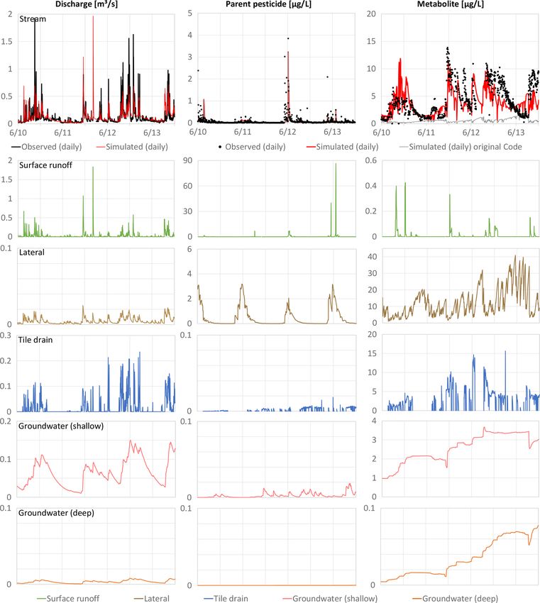
160                                   H. Rathjens et al.: Technical note: Extending the SWAT model to transport chemicals

relevant when simulating more stable, soluble, and mobile            2.2   Description of the new subsurface transport
pesticides or metabolites (or other stable and mobile con-                 functionality
stituents and tracers), when working in environments with a
strong interaction between surface water and groundwater, in         SWAT’s source code (publicly available at https://bitbucket.
regions with shallow groundwater tables, and in areas where          org/blacklandgrasslandmodels/swat_development, last ac-
tile drains exist.                                                   cess: 5 January 2023; this study is based on version 681) con-
   The model extension presented here fills this gap by con-         sists of around 300 individual Fortran subroutines in which
sidering pesticide transport through tiles and groundwater re-       the processes and the functional modeling workflow are im-
turn flow to surface waterbodies in SWAT.                            plemented. This modular structure allows the implementa-
                                                                     tion of new functionalities through adding new routines or
                                                                     the modification of single subroutines.
2     Software description                                              Figure 1 shows a schematic representation of the newly
                                                                     implemented SWAT pesticide routing scheme. The current
2.1    SWAT model structure                                          version of the SWAT model prevents soluble pesticides from
                                                                     leaching out of the soil profile (which includes the root zone
The structure of the SWAT model allows for the prediction
                                                                     below the maximum soil depth). Chemicals are prevented to
of flow, sediment, nutrients, and pesticide fluxes at multi-
                                                                     flow through tile drains or entering the groundwater. While
ple scales and locations throughout a watershed. The SWAT
                                                                     the tile and groundwater flow along with several loadings
model divides the catchment into multiple subbasins. Sub-
                                                                     (e.g., nutrients) are simulated, the pesticide load is not routed.
basin delineation is based on the size of the catchment and
                                                                     Thus, subroutines simulating subsurface flow and transport
the density of the stream network. Subbasins are created
                                                                     processes were modified to enable pesticide flux together
when two streams merge and can manually be added to rep-
                                                                     with the tile flow and groundwater flows. The tile drain pes-
resent each point where model predictions are required. A
                                                                     ticide routing calculations were implemented in the pesticide
subbasin is divided into multiple hydrologic response units
                                                                     leaching routine (pestlch.f) and a newly introduced subrou-
(HRUs), which are representative of unique combinations
                                                                     tine (pestgw.f) contains the algorithms to simulate pesticide
of land use, soils, and slope within a subbasin. Each HRU
                                                                     transport via shallow and deep groundwater flows.
is considered an independent land unit within SWAT, and
each HRU can have different parameterizations and agro-              2.3   Tile drain flow pesticide implementation
nomic practices, including tile drains. Within the soil lay-
ers of an HRU, fluxes are distinguished into surface runoff,         Vertical and lateral pesticide movement within the soil layer
lateral flow, and tile flow (if tile drains are present) that con-   as well as percolation out of the soil layer is calculated in sub-
tribute to streams. Additionally, evaporation and recharge to        routine pestlch.f. For adding the capability of routing pesti-
groundwater occur. In up to two groundwater aquifers, the            cide through tile drains, corresponding equations were added
incoming water is partitioned into capillary rise (re-entering       to this subroutine. First, if tile drains are implemented in the
the soil profile from the shallow groundwater layer), storage,       respective soil layer, tile flow is added to the water that is
percolation, or outflow to streams. The second aquifer can           leaving the layer (Eq. 1):
either be unconnected (fluxes are lost from the system) or
connected (fluxes are routed back to the streams). All out-          qlyr = qtile + qprk + qlat ,                                   (1)
going HRU fluxes enter the streams at the upstream end of
the segment and are routed to the downstream end, during             where qlyr is the pesticide transport-effective flow leaving
which in-stream processes such as attenuation, partitioning,         the tile-drained soil layer (without evaporation or plant up-
and degradation take place. The timing of HRU-level fluxes           take) (mm H2 O), qtile is the tile flow leaving the soil layer
entering an associated stream is a function of the subbasin          (mm H2 O), qprk is the percolation out of the layer (mm H2 O),
time of concentration and does not vary across HRUs. The             and qlat is the lateral flow leaving the soil layer (mm H2 O).
process of a parent chemical forming a metabolite is not im-         Based on qlyr , the amount of soluble pesticide leaving the
plemented in the current SWAT version. Thus, the metabolite          tile-drained soil layer is calculated with Eq. (2) for each pes-
formation requires a separate calculation and implementation         ticide (see Neitsch et al., 2011, Chapter 4:3, and Leonard et
in the model using “pseudo” chemical applications. For fur-          al., 1987):
ther information on the calculation of fluxes and concentra-                                         qlyr
tions of constituents, the reader is referred to the SWAT the-                                −
                                                                     pstrem = solpst · 1 − e wsat +fads ·solbd ·sold ,            (2)
oretical documentation (Neitsch et al., 2011).
                                                                     where pstrem is the total amount of soluble pesticide removed
                                                                     from the soil layer (kg ha−1 ), solpst is the initial amount of to-
                                                                     tal pesticide in the soil layer (kg ha−1 ), wsat is the amount of
                                                                     water in the soil layer at saturation (mm H2 O), fads is the soil

Hydrol. Earth Syst. Sci., 27, 159–167, 2023                                              https://doi.org/10.5194/hess-27-159-2023
H. Rathjens et al.: Technical note: Extending the SWAT model to transport chemicals 161
Figure 1. Flow chart of the newly implemented pesticide routing functionality.
adsorption coefficient (mg kg−1 /mg L−1 ), solbd is the soil where pstshallst and pstshallst–1 denote the amount of pesticide
bulk density of the soil layer (mg m−3 ), and sold is the depth stored in the shallow aquifer on the present and previous day
of the soil layer (mm). Pesticide concentration in tile flow is (kg ha−1 ), respectively. Then, the pesticide groundwater con-
then calculated by dividing the amount of removed pesticide tribution to streamflow is calculated as follows:
through the flow leaving the layer (Eq. 3): pstshallst
pstshallconc = , (7)
pstrem dshall · fpstgw + qgwshall + revap + qgwseep
pstconc = , (3)
qtile + qprk + qlat pstgwshall = pstshallconc · qgwshall , (8)
where pstconc is the concentration of pesticide in the where pstshallconc is the pesticide concentration in shallow
water (including the tile flow) leaving the soil layer aquifer groundwater (mg ha−1 mm−1 ), dshall is the depth of
(kg ha−1 mm−1 ). Finally, Eq. (4) is then as follows: water in the shallow aquifer (mm H2 O), fpstgw is the shal-
psttile = pstconc · qtile , (4) low groundwater pesticide mixing factor (dimensionless),
qgwshall is the shallow groundwater contribution to stream-
where psttile is the amount of pesticide leaving the soil layer flow (mm H2 O), revap is the amount of water moving from
through tile flow (kg ha−1 ). the shallow aquifer into the soil profile or being taken up by
plant roots in the shallow aquifer (mm H2 O), qgwseep is the
2.4 Groundwater flow pesticide implementation
amount of water recharging the deep aquifer, and pstgwshall
The newly introduced subroutine pestgw.f contains equations is the amount of pesticide entering the channel via shallow
to calculate pesticide transport via groundwater. First, the aquifer groundwater flow (kg ha−1 ). The amount of pesticide
amount of pesticide in the shallow aquifer is calculated with in the shallow aquifer is then updated as follows:
Eq. (5): pstgwseep = pstshallconc · qgwseep , (9)
pstrchrg = 1 − e−1.0/gwdelay · pstsol
pstshallst = pstshallst–1 − pstgwshall − pstgwseep , (10)
−1.0/gwdelay
+e · pstrchrg–1 , (5) where pstgwseep is the amount of pesticide recharging into the
where pstrchrg is the amount of pesticide entering the shal- deep aquifer (kg ha−1 ). The deep aquifer pesticide contribu-
low aquifer (mg ha−1 ), gwdelay is the time required for water tion to streamflow is then calculated as follows:
and its soluble loadings to reach the shallow aquifer from the pstdeepst = pstdeepst–1 + pstgwseep , (11)
bottom of the root zone (d), pstsol is the daily amount of pes- pstdeepst
ticide leached from the soil profile (mg ha−1 ), and pstrchrg–1 pstdeepconc = , (12)
is the amount of pesticide entering the shallow aquifer on ddeep · fpstgwdeep + qgwdeep
the previous day (mg ha−1 ). The current pesticide mass is pstgwdeep = pstdeepconc · qgwdeep , (13)
tracked with Eq. (6):
where pstdeepst and pstdeepst–1 denote the amount of pesti-
pstshallst = pstshallst–1 + pstrchrg , (6) cide stored in the deep aquifer on the present and previ-
https://doi.org/10.5194/hess-27-159-2023 Hydrol. Earth Syst. Sci., 27, 159–167, 2023162 H. Rathjens et al.: Technical note: Extending the SWAT model to transport chemicals
ous day (kg ha−1 ), respectively, pstdeepconc is the pesticide Model parameterization followed standard procedures
concentration in deep aquifer groundwater (mg ha−1 mm−1 ), considering information on climate, topography, soil, land
ddeep is the depth of water in the deep aquifer (mm H2 O), use properties, agricultural management practices (includ-
fpstgwdeep is the deep groundwater pesticide mixing factor ing pesticide applications), and tile drain locations. SWAT
(dimensionless), qgwdeep is the deep groundwater contribu- offers a range of algorithms representing hydrological pro-
tion to streamflow (mm H2 O), and pstgwdeep is the amount cesses. Based on experience and understanding of the catch-
of pesticide entering the channel via deep aquifer groundwa- ment characteristics, the Hargreaves potential evaporation
ter flow (kg ha−1 ). Finally, the pesticide amount in the deep method and the evaporation-based daily curve number ad-
aquifer is updated: justment method were chosen. Pre-calibration settings of hy-
drologic parameters included the adjustment of heat units
pstdeepst = pstdeepst–1 − pstgwdeep . (14) to ensure crops develop completely and the adjustment of
channel roughness to account for vegetated, small channels.
In addition, minor changes were made to other subroutines
Application data on respective crops were available with ap-
for technical reasons, e.g., to produce HRU-level output,
proximate amounts and timing for C1 and as field-specific
track pesticide fluxes in all flow components, and write the
applications for C2. The pesticide’s average application rates
fluxes to output files. These changes are not discussed here
are 221 g ha−1 in C1 and 462 g ha−1 in C2. Metabolite re-
but are included in the code provided in the electronic sup-
lease in the soil was parameterized to account for metabo-
plements.
lite formation in the soil profile using pseudo chemical ap-
The model will be largely compatible with the input files
plications for both model versions. Pesticide-related algo-
of the original SWAT code. The only change required to the
rithms and parameters updated prior to calibration included
default SWAT input parameters is the addition of the ground-
pesticide in-stream processes such as burial and volatiliza-
water mixing parameters in the basins.bsn input file. These
tion, which were turned off due to the low Koc, Henry’s law
two parameters must be added to line 136 and 137 of the
constant, and vapor pressure of both chemicals and the short
basins.bsn input file manually and have the following default
travel time in the two catchments.
values:
A multi-metric calibration was conducted combining vi-
1.0000 |PESTGWFACTOR: mixing factor of pesticide en-
sual comparison and multiple performance metrics for both
tering shallow gw aquifer – 0 no mixing, 1 complete and in-
streamflow and concentration of the chemicals using the
stantaneous mixing.
modified SWAT code. The calibration was conducted sepa-
1.0000 |PESTGW_D_FACTOR: mixing factor of pesticide
rately and iteratively for streamflow and pesticide concen-
entering deep aquifer – 0 no mixing, 1 complete and instan-
trations (i.e., no multi-objective function combining stream-
taneous mixing.
flow and pesticide metrics was used). The entire record of ob-
A compiled Windows executable and the complete model
served chemical concentrations was selected as the calibra-
code are provided as electronic supplements.
tion period and a second independent validation period was
not selected. This is a common approach used for hydrologic
3 Application and pesticide model calibration when the observed data pe-
riod is relatively short (Daggupati et al., 2015). The models
Application of the modified SWAT model was conducted in for the two watersheds were first calibrated using the modi-
two agricultural catchments in Western Europe. The catch- fied code and then both model versions (original and modi-
ment characteristics are summarized in Table 1. Catchment fied) were run using the same parameters. This is not meant
names and location as well as detailed descriptions and to be a completely “equitable” model performance compar-
names of the chemicals were anonymized for this publi- ison, but to show the differences between the two versions.
cation. In both catchments, pesticide application data were A list and description of the calibration parameters and the
available along with observations of streamflow, pesticide, processes they are associated with is provided in Table 2. A
and pesticide metabolite concentrations. All data sources parameter is included in the table if it was changed in at least
overlap temporally from June 2016 to December 2019 for one of the catchments.
catchment 1 (C1) and from June 2010 to December 2013 Figures 2 and 3 show discharge, pesticide, and metabo-
for catchment 2 (C2). The parent pesticide is a commonly lite concentrations (columns) for the different flow compo-
used chemical typically applied in late autumn on winter nents (rows) for C1 and C2, respectively. The hydrologic cal-
grains or in spring on corn. Based on the pesticide’s soil ibration led to a good visual agreement between observed
half-life (approximately 6 to 40 d, depending on soil type; and simulated discharge and good to very good performance
Bayer Crop Science, 2018), it is classified as “readily degrad- statistics with daily NSE values of 0.76, 0.63 and PBIAS of
able”, its mobility is classified as “moderate”, and it is con- 6.6 %, 1.8 % in C1 and C2, respectively. The pesticide and
sidered “readily soluble” in water (Koc of ∼ 250 mL g−1 ). metabolite concentrations in streamflow simulated with the
In contrast, the metabolite is stable, “highly mobile” (Koc of original SWAT code (gray lines) and the modified code (red
0 mL g−1 ), and “highly soluble” (FAO, 2000). lines) are shown in Figs. 2 and 3. The original and modi-
Hydrol. Earth Syst. Sci., 27, 159–167, 2023 https://doi.org/10.5194/hess-27-159-2023H. Rathjens et al.: Technical note: Extending the SWAT model to transport chemicals 163
Table 1. Catchment characteristics of the two anonymized catchments in Western Europe.
Catchment characteristics Unit Catchment 1 Catchment 2
Catchment area at gauge km2 38.0 9.9
Elevation gradient m a.s.l. 45–110 24–159
Land use distribution – Agriculture (73 %) Agriculture (80 %)
Forest (17 %) Pasture (13 %)
Urban (10 %) Forest (6 %)
Pasture (2 %)
Tile drained % 52 48
Average annual precipitation (min–max)∗ mm 641–809 631–945
Average annual maximum temperature (min–max)∗ ◦C 13.1–15.6 13.3–15.4
Average annual minimum temperature (min–max)∗ ◦C 4.3–6.1 5.6–7.1
Mean runoff rate as percent of precipitation∗∗ % 28–36 38–48
Number of subbasins – 39 17
Number of HRUs – 5163 922
∗ Time period: January 2008 to December 2013, ∗∗ time period: June 2010 to December 2013.
Table 2. Calibration parameters with initial value and calibrated end value (changed values in bold).
SWAT parameter Parameter description Initial value Calibrated end value
C1 C2
Surface runoff CNCOEF Plant ET curve number coefficient 1 1.1 1
SURLAG Surface runoff lag coefficient 1 1 0.5
Tile drains DEPIMP Depth to restrictive layer (mm) n/a∗ 2010 2250
GDRAIN Drain tile lag time (h) 0 2 12
TDRAIN Time for tiles to drain soil to field 48 48 24
capacity (h).
DDRAIN Depth to subsurface tile drain (mm) 1000 990 1000
Groundwater ALPHA_BF Baseflow alpha factor 0.048 0.77 0.01
GWDELAY Groundwater delay (d) 31 47.4 1
ALPHA_BF_D Baseflow alpha factor for deep aquifer 0.01 0.01 0.0001
GWQMIN Threshold depth of water in the shallow 1000 1000 500
aquifer required for return flow (mm)
RCHRG_DP Deep aquifer percolation fraction 0.05 0.05 0.15
Soil AWC Available water capacity default by soil 1.1*default 1.33*default
ESCO Soil evaporation compensation factor 0.95 0.95 1
Pesticide and PERCOP Pesticide percolation coefficient 0.5 0.5 0.6
Metabolite PESTGWFACTOR Mixing ratio of pesticide entering shallow 1 1 0.02
gw aquifer
PEST_GW_D Mixing ratio of pesticide entering deep 1 0.02 1
gw aquifer
∗ n/a stands for not applicable.
fied SWAT pesticide simulations returned similar results and not included in the model; this leads to discrepancies be-
a good fit between modeled and observed concentrations was tween simulated and observed concentrations. The metabo-
achieved. However, C1 was characterized by very few detec- lite dynamics and magnitudes cannot be reproduced by the
tions above the level of quantification and the highest ob- original SWAT code in both catchments, but are very well
served pesticide peak could not be reproduced by both mod- represented by the modified code, emphasizing the impor-
els. In C2, reported point source inputs of the pesticide oc- tance of the subsurface transport processes for the metabo-
curred (likely due to mistreatment of the product) which are lite.
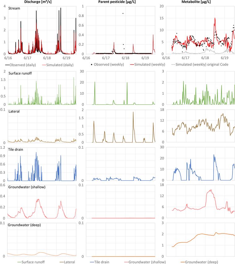
https://doi.org/10.5194/hess-27-159-2023 Hydrol. Earth Syst. Sci., 27, 159–167, 2023164 H. Rathjens et al.: Technical note: Extending the SWAT model to transport chemicals Figure 2. Catchment 1 (C1) time series (June 2016–December 2019) for observed and simulated discharge, parent pesticide, metabolite in streamflow and simulated time series for all flow components. The contribution of the different flow components to dis- rably high pesticide concentrations in streamflow coincide charge is similar in both catchments where surface runoff with a significant runoff event. Pesticide concentrations in has the highest impact on peak flows. Tile drains are rele- lateral flow are also significant, but the contribution of lateral vant mostly in the wetter months and shallow groundwater flow to total streamflow is low, and loadings in lateral flow shows a clear seasonal dynamic with lowest flow values in are therefore significantly diluted when entering the stream. summer. Lateral flow and deep groundwater flow have low The concentrations of the metabolite in streamflow have a contributions. The deep groundwater aquifer, however, sus- comparable magnitude in C1 and C2 (maximum between 10 tains the flows in the summer periods. The modified SWAT to 15 µg L−1 ) and the dynamics of the concentrations in the code allows the output of concentrations in all flow compo- transport components have a similar pattern in both catch- nents. They show a similar pattern in both catchments where ments. Concentrations in lateral flow fluctuate, but are al- surface runoff and lateral flow are the only flow compo- ways greater than zero, indicating a constant presence of the nents with significant concentrations. All simulated pesticide metabolite in the soil. This can also be seen in the high tile peaks can be attributed to surface runoff events as compa- drain concentrations that lead to substantial metabolite con- Hydrol. Earth Syst. Sci., 27, 159–167, 2023 https://doi.org/10.5194/hess-27-159-2023
H. Rathjens et al.: Technical note: Extending the SWAT model to transport chemicals                                               165

Figure 3. Catchment 2 (C2) time series (June 2010–December 2013) for observed and simulated discharge, parent pesticide, metabolite in
streamflow and simulated time series for all flow components.

tributions when tile flow occurs. The metabolite is also per-        4   Summary and conclusion
manently present in the groundwater, which is a significant
transport pathway.                                                   The SWAT model code was extended to simulate pesticide
   These results show that the fast flow components are re-          transport through tile drains and two groundwater layers. All
sponsible for the pesticide concentrations in streamflow. For        subroutines and a compiled executable are provided in the
the metabolite, a single most important transport process can-       electronic supplements to this technical note. For applying
not be identified and a complex interplay between multiple           the updated model, minor changes must be made to the stan-
transport pathways is responsible for the concentration dy-          dard SWAT input files with two additional parameters in one
namics and magnitude: lateral flow and shallow groundwater           input file.
flow are the most important input pathways in summer dur-               The application of the implemented code in the two case
ing low flow conditions and tile drain flow during autumn            study catchments demonstrates the advantages to simulating
and winter. Surface runoff and deep groundwater flow have            pesticide transport through tile drains and groundwater flow.
negligible contributions.                                            The actual concentrations in the respective transport path-

https://doi.org/10.5194/hess-27-159-2023                                             Hydrol. Earth Syst. Sci., 27, 159–167, 2023
166                                     H. Rathjens et al.: Technical note: Extending the SWAT model to transport chemicals

ways and water balance components are available over time;               Financial support. This research has been supported by Bayer.
this is important information to assess environmental fate
and transport processes. It is also apparent that the complex
temporal interplay between all flow components, including                Review statement. This paper was edited by Micha Werner and re-
tile and groundwater flow, is needed to sufficiently simulate            viewed by two anonymous referees.
concentrations of metabolites and other chemicals with sim-
ilar properties in streamflow. Visualizing the pesticide and
metabolite concentration in all flow components improves                 References
the understanding of the origin of the chemicals. This sup-
ports a more targeted calibration of the models and provides             Arabi, M., Frankenberger, J. R., Engel, B., and Arnold, J. G.: Repre-
important information to develop best management practices                 sentation of agricultural management practices with SWAT, Hy-
to mitigate potential contamination of surface and groundwa-               drol. Process., 22, 3042–3055, 2008.
ter.                                                                     Arnold, J. G., Srinivasan, R., Muttiah, R. S., and Williams, J. R.:
   The developed software fills a gap in watershed-scale pes-              Large-area hydrologic modeling and assessment: part I. model
ticide modeling. The code refinements were made available                  development, Am. Wat. Res., 34, 73–89, 1998.
                                                                         Bannwarth, M. A., Sangchan, W., Hugenschmidt, C., Lamers, M.,
to the SWAT development team and will potentially be in-
                                                                           Ingwersen, J., Ziegler, A. D., and Streck, T.: Pesticide transport
cluded in a future official revision of the SWAT model. The                simulation in a tropical catchment by SWAT, Environ. Pollut.,
next version of the SWAT model, called SWAT+ (Bieger et                    191, 70–79, 2014.
al., 2017), will include the simulation of pesticides in all hy-         Bayer Crop Science: Bayer Crop Science Internal Report 1, 144 pp.,
drological flow pathways and a direct simulation of metabo-                2018.
lite formation using a first-order decay function. However,              Bieger, K., Arnold, J. G., Rathjens, H., White, M. J., Bosch, D.
while scientists and watershed managers are in the process                 D., Allen, P. M., Volk, M., and Srinivasan, R.: Introduction to
of transitioning to SWAT+ and its supporting interfaces be-                SWAT+, A Completely Restructured Version of the Soil and Wa-
come available, the extended SWAT version is a valuable tool               ter Assessment Tool, J. Am. Water Resour. As., 53, 115–130,
for risk managers and exposure modelers.                                   https://doi.org/10.1111/1752-1688.12482, 2017.
                                                                         Daggupati, P., Pai, N., Ale, S., Douglas-Mankin, K. R., Zeckoski, R.
                                                                           W., Jeong, J., Parajuli, P. B., Saraswat, D., and Youssef, M. A.:
                                                                           A recommended calibration and validation strategy for hydraulic
Code availability. The source code and compiled Windows exe-
                                                                           and water quality models, T. ASABE, 58, 1705–1719, 2015.
cutables are available from Stone Environmental’s GitHub reposi-
                                                                         FAO: Assessing soil contamination, A reference manual, FAO Pesti-
tory (https://github.com/StoneEnv/SwatPestTileGw; Rathjens et al.,
                                                                           cide disposal series 8, Food and Agricultural Organization of the
2023) under the GNU General Public License v3.
                                                                           United Nations, https://www.fao.org/3/X2570E/X2570E00.htm#
                                                                           TOC, last access: January 2022.
                                                                         Fohrer, N., Dietrich, A., Kolychalow, O., and Ulrich, U.: Assess-
Author contributions. HR, MW, and RS conceptualized the re-                ment of the Environmental Fate of the Herbicides Flufenacet and
search. JK, HR, MW, and RS curated and processed the data. HR,             Metazachlor with the SWAT Model, J. Environ. Qual., 43, 75–85,
JK, and MW developed the methodology. JA, HR, and MW devel-                2014.
oped the software. RS supervised the study. JK, HR, and MW ap-           Gassman, P. W., Reyes, M. R., Green, C. H., and Arnold, J. G.: The
plied the model and validated the results. JK visualized the data.         Soil and Water Assessment Tool: Historical development, appli-
JK wrote the initial draft of the manuscript. All authors reviewed,        cations, and future research directions, T. ASABE, 50, 1211–
commented and edited the manuscript.                                       1240, 2007.
                                                                         Gassman, P. W., Sadeghi, A. M., and Srinivasan, R.: Applications
                                                                           of the SWAT Model Special Section: Overview and Insights, J.
Competing interests. The contact author has declared that none of          Environ. Qual., 43, 1–8, 2014.
the authors has any competing interests.                                 Holvoet, K. A., Gevaert, V., van Griensven, A., Seuntjens, P., and
                                                                           Vanrolleghem, P. A.: Modeling the effectiveness of agricultural
                                                                           measures to reduce the amount of pesticides entering surface wa-
Disclaimer. Publisher’s note: Copernicus Publications remains              ters, Water Resour. Manag., 21, 2027–2035, 2007.
neutral with regard to jurisdictional claims in published maps and       Leonard, R. A., Knisel, W. G., and Still, D. A.: GLEAMS: Ground-
institutional affiliations.                                                water loading effects on agricultural management systems, T.
   The authors accept no responsibility for any liability arising from     ASAE, 30, 1403–1428, 1987.
the use of this manuscript, the provided source code and model.          Neitsch, S. L., Arnold, J. G., Kiniry, J. R., and Williams, J. R.:
                                                                           Soil and Water Assessment Tool theoretical documentation, Ver-
                                                                           sion 2009, TX Water Res. Inst. Tech. Rep. no. 406, College
Acknowledgements. We acknowledge and thank Bayer AG Divi-                  Station (TX), USA, 647 pp., https://swat.tamu.edu/media/99192/
sion Crop Science for funding the work.                                    swat2009-theory.pdf (last access: January 2023), 2011.
                                                                         Quilbe, R., Rousseau, A. N., Lafrance, P., Leclerc, J., and Amrani,
                                                                           M.: Selecting a Pesticide Fate Model at the Watershed Scale Us-

Hydrol. Earth Syst. Sci., 27, 159–167, 2023                                                  https://doi.org/10.5194/hess-27-159-2023
H. Rathjens et al.: Technical note: Extending the SWAT model to transport chemicals 167 ing a Multi-criteria Analysis, Water Qual. Res. J. Can., 41, 283– Winchell, M. F., Peranginangin, N., Srinivasan, R., and Chen, W.: 295, 2006. Soil and Water Assessment Tool Model Predictions of Annual Rathjens, H., Winchell, M., and Arnold, J.: SWAT code capable Maximum Pesticide Concentrations in High Vulnerability Wa- to route chemicals through tile drains and groundwater, GitHub tersheds, Integr. Environ. Asses., 14, 358–368, 2018. [code]:, https://github.com/StoneEnv/SwatPestTileGw, last ac- Zhang, X. and Zhang, M.: Modeling effectiveness of agricultural cess: January 2023. BMPs to reduce sediment load and organophosphate pesticides Vazquez-Amabile, G., Engel, B. A., and Flanagan, D. C.: Modeling in surface runoff, Sci. Total Environ., 409, 1949–1958, 2011. and risk analysis of nonpoint source pollution caused by atrazine using SWAT, T. ASABE, 49, 667–678, 2006. https://doi.org/10.5194/hess-27-159-2023 Hydrol. Earth Syst. Sci., 27, 159–167, 2023
You can also read