Oxygen transport during liquid ventilation: an in vitro study - Nature
←
→
Page content transcription
If your browser does not render page correctly, please read the page content below
www.nature.com/scientificreports
OPEN Oxygen transport during liquid
ventilation: an in vitro study
Katrin Bauer1*, Thomas Janke2 & Rüdiger Schwarze1
An in vitro experiment on the dissolved oxygen transport during liquid ventilation by means of
measuring global oxygen concentration fields is presented within this work. We consider the flow
in an idealized four generation model of the human airways in a range of peak Reynolds numbers of
Re = 500–3400 and Womersley numbers of α = 3–5. Fluorescence quenching measurements were
employed in order to visualize and quantify the oxygen distribution with high temporal and spatial
resolution during the breathing cycle. Measurements with varying tidal volumes and oscillating
frequencies reveal short living times of characteristic concentration patterns for all parameter
variations. Similarities to typical velocity patterns in similar lung models persist only in early phases
during each cycle. Concentration gradients are quickly homogenized by secondary motions within
the lung model. A strong dependency of peak oxygen concentration on tidal volume is observed with
considerably higher relative concentrations for higher tidal volumes.
Since its first mention in 1962 by Kylstra et al.1, Liquid Ventilation (LV) has been proposed as a promising ven-
tilation strategy for various complications occurring in intensive care. Greenspan et al.2 suggested the treatment
of preterm neonates with a LV protocol. They could show an improvement in lung function and underlined the
advantages of the utilized perfluorocarbon (PFC) liquids (high gas solubility, low surface tension, distributes
evenly). Furthermore, liquid ventilation has also been proposed to treat adult patients with acute respiratory dis-
tress syndrome (ARDS)3. But until today, liquid ventilation lacks a proof of performing better than conventional
mechanical ventilation (CMV)4 for this case. More recent studies suggest to incorporate hypothermic total liquid
ventilation (TLV) after cardiac a rrest5–9. Such a protocol has not only the advantage of providing ventilation for
the patient but it can also protect the cardio- and neurosystem by ultra-fast cooling. To do so, a body temperature
of around 33 ◦ C (mild hypothermia) has to be achieved within the shortest time possible. As Chenouve et al.5
showed, cooling by TLV can be three to four times faster in comparison to conventional cooling strategies. From
a fluid dynamic perspective, liquid ventilation has just been sparsely investigated. While the results of researches
concerning the fluid’s behavior during gas ventilation may be transferable to liquid ventilation strategies based
on comparable characteristic numbers (Reynolds number, Womersley number), only a few dedicated studies
have been published in order to gain new insights into the processes of liquid ventilation. Some of these studies
have been summarized by Halpern et al.10. This review mainly covers the transport of liquid plugs in confined
channels. Such process may be most important during filling of the lungs. After successful administration of
the liquid, the transport mechanisms of dissolved gases play a crucial major role for providing enough fresh
oxygen. While a few approaches have been taken of imaging the oxygen distribution within the lungs11–14, they
are all limited by the achievable spatial resolution and mainly the determination, whether certain regions are
preferably supplied with PFC or not. Within the work here presented, we want to introduce an in vitro study on
the dissolved oxygen transport and distribution modeling the flow within the conductive airways of the human
lung. First experiments have been presented in the past by our group15,16. Within these works, we investigated
dissolved oxygen concentrations during constant inspiration and expiration and could identify characteristic
distribution patterns. In this new work, we investigate the influence of oscillatory flow on the distribution and
transport patterns during different phases of the breathing cycle.
Methods
Lung model. The model features four symmetrical airway generations with circular cross sections. The
geometry is based on the model presented in17 as flow visualization measurements, i.e. particle image veloci-
metry (PIV) measurements have been carried out in the similar geometry. Starting from the largest channel
( D1 = 10.48 mm), it bifurcates three times and the channel’s diameter reduces down to ( D3 = 3.3 mm) as mini-
mum diameter (see Fig. 1a). With these dimensions it hence represents an adult lung from approximately the
2nd to the 5th bifurcating generation , featuring a model dead space of about 10 ml . The experimental model
1
Institute of Mechanics and Fluid Dynamics, TU Bergakademie Freiberg, Freiberg, Germany. 2LaVision, Göttingen,
Germany. *email: Katrin.Bauer@imfd.tu-freiberg.de
Scientific Reports | (2022) 12:1244 | https://doi.org/10.1038/s41598-022-05105-1 1
Vol.:(0123456789)
www.nature.com/scientificreports/
Model generation i Di (mm) li (mm) αi (°)
0 10.48 47.6
1 7.86 22.6 64
2 4.98 9.22 66
3 3.3 6.72 68
Table 1. Geometrical characteristics of the simplified lung model.
(a) (b)
10 mm Di
lung
model
li
i
syringe pump
Figure 1. (a) Geometry of the lung model, (b) sketch of the experimental set-up illustrating the flow paths
between the syringe pump and the storage liquid containers. Red colors denote initial high concentration, blue
low concentration, purple is a mixed concentration.
is made of polymethyl methacrylate (PMMA) and nine hose connectors are attached, one at the largest channel
and eight at the distal ends. All relevant geometrical dimensions are given in Table 1.
Model limitations. The lung model employed here with flat, symmetric bifurcations features a strong simplifi-
cation of the real lung. Thus, additional rotations of the Dean vortices, which can be observed in a fully three-
dimensional model geometry18 , cannot be generated here. Due to the rigid structure any compliances as well
as collapsible structures can also not be considered here. However, the geometry is sufficient to cover the main
features of convective lung flow and gas transport. The big advantage of planar lung models is the option of a
simultaneous optical flow analysis of all mother and daughter branches. The round cross sections and bifurcat-
ing branches thus allow the generation of the characteristic Dean vortex patterns, typical flow split-up as well
as skewed velocity p rofiles19 . By variation of the breathing parameters, laminar as well as turbulent flow condi-
tions can be covered here. The simplified geometry hence allows a better systematic study of flow induced gas
concentration and mixing patterns.
Experimental set‑up. The lung model is fixed horizontally on an optical bench. It is connected to a syringe
pump and three liquid storage containers via several flexible hoses. Two different flow paths are needed to sup-
ply the model with liquid of high or low oxygen concentration during inspiration and expiration, respectively.
This is achieved with Y-connectors and non-return valves (see Fig. 1b). Two of the storage containers are used
to supply the model with liquid of initially low and high concentrations, respectively, while the third acts as an
overflow tank.
The syringe pump consists of a linear actuator (LinMot) driving four syringes. The linear motor follows a
sinusoidal motion with adjustable stroke and frequency. Two of the four syringes are grouped to either contribute
to the inspiration or the expiration phase, respectively. While the syringes push liquid with high oxygen con-
centration (red arrow) through the model during inspiration, liquid of low oxygen concentration (blue arrow)
is pulled from a storage container through the eight distal channels during expiration. The determination of the
dissolved oxygen concentration fields is carried out for six different tidal volumes ( Vt = 30, 40, 50, 60, 80, 100 ml)
and three oscillation frequencies of f = 0.05 Hz, 0.1 Hz and 0.15 Hz , i.e. 3, 6 and 9 ventilation cycles per
minute. The tidal volumes cover a range of 3–10 times of the model dead space which is about 10 ml. As real
lungs have a typical dead space of 150 ml and tidal volume during normal breathing is about 500 ml, total liq-
uid ventilation typically covers about 1000 ml (15–20 ml/kg bodyweight) of tidal v olume2. Hence, the ratio of
tidal volume to dead space of our model agrees to physiological conditions. The ventilation frequencies applied
here correspond to the frequency range of total liquid ventilation with 3–8 cycles per minute2,20 . The peak
Reynolds number during the breathing cycle is given by Re = 4VT ρ f /D0 µ (at peak velocity in the trachea);
the corresponding Womersley number capturing unsteady inertial effects due to oscillatory motion is defined
as α = D0 /2 2π f ρ/µ . Here, the values for the density ρ and dynamic viscosity µ are based on the values of
water with ρ = 1000 kg/m3 and µ = 1 · 10−3 Pa · s . All relevant flow parameters are summarized in Table 2.
Scientific Reports | (2022) 12:1244 | https://doi.org/10.1038/s41598-022-05105-1 2
Vol:.(1234567890)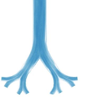
www.nature.com/scientificreports/
f (Hz) VT (ml) umax (m/s) Re 0 α
0.05 30 0.054 572 2.9
0.1 30 0.109 1145 4.2
0.15 30 0.164 1717 5.1
0.05 40 0.073 673 2.9
0.05 50 0.091 954 2.9
0.05 60 0.109 1145 2.9
0.1 60 0.219 2290 4.2
0.15 60 0.328 3435 5.1
0.05 80 0.146 1526 2.9
0.05 100 0.182 1908 2.9
Table 2. Variation of flow parameters. Velocity, Reynolds numbers Re and Womersley numbers α,
representing peak values in the 0th generation.
This overview shows that the full range from laminar to turbulent flow conditions as well as typical physiological
Womersley numbers are covered here.
Oxygen concentration measurements. The measurements of the dissolved oxygen concentration are
based on the oxygen quenching characteristics of the metallic complex Dichlorotris(1,10)-(phenanthroline)
ruthenium(II) ([Ru(phen)3]2+). The complex is solved in ethanol (0.4 g:400 ml) and further mixed with 3.6 l of
water. This final water-ethanol-dye solution is used as the working fluid during the experiments and also acts
as a sensor liquid at the same time. As we showed in a previous work16, there are just little differences between
using water or an actual PFC liquid in the found concentration maps. The local oxygen concentration is then
visualized by the local fluorescence intensity of the working fluid. A higher oxygen concentration is thus associ-
ated with a lower fluorescence intensity. The field of view is imaged with a charged coupled device (CCD) camera
(monochrome, resolution after pixel binning: 800 × 150 px, exposure time: 500 µs, pco.1600). Illumination is
provided by a pulsed high-power LED ( = 455 nm, pulse-length: 450 µs, PT-120, Luminus). A volumetric
illumination is applied here. That means, the camera, in top view, acquires an integral image of the fluorescence
intensity and not values of the cross sectional mid plane. The excitation wavelengths of the LED are separated
from the emission wavelengths of the sensor liquid by an optical high-pass filter ( cut = 550 nm) placed in front
of the camera’s CCD chip.
A calibration of the sensor liquid is necessary in order to convert the measured intensity distributions of
recorded images into physical oxygen concentrations via the Stern–Volmer equation.
Iref
= KSV · [O2 ] + 1 (1)
I
The calibration is performed prior to the experiments by filling the model with the sensor liquid at ten known
oxygen concentrations. The reference probe used here is a dissolved oxygen meter (GMH 3611, Greisinger).
The Stern–Volmer constant is then determined by a linear regression of the known intensity-concentration cor-
respondences. The calibration yields a Stern–Volmer constant of KSV = 0.1127 ± 0.002 l/mg at a temperature
of 18.5 ◦C.
In order to model the effect of inspiration and expiration, the liquid in one of the storage containers is
enriched with oxygen, while the liquid in the other one is degassed by stripping with nitrogen. The dissolved
oxygen concentrations are adjusted to stay at approximately 1 mg/l in the low oxygen concentration tank and at
around 8–9 mg/l in the oxygen enriched tank. The liquid’s temperature was constant at 19 ± 0.5 ◦ C. Due to the
maximum liquid storage volume of the tanks with 4 l, the number of periodic cycles is limited and depends on
the investigated tidal volume. Thus, we can record between ten and twenty full breathing cycles. Both, camera
and LED are triggered at pre-defined positions of the linear actuator, which enables us to perform phased-locked
recordings. The presented results of these measurements are all based on the phase averaging over the total
number of recorded breathing cycles. Relative uncertainties of the phase averaged concentrations were found to
be in the order of 0.01–0.7%. Altogether, 32 phase positions were measured here.
Results and discussion
Qualitative concentration distribution. At first, we present qualitative concentration visualization
results with the aim of identifying important mass transport characteristics. The results are shown for an oscil-
lation frequency of f = 0.05 Hz and a tidal volume of 60 ml. Eight phase positions during the whole breathing
cycle are included in Fig. 2. The upper part represents the inhalation cycle from the acceleration (ϕ = 1/4π )
until the flow reversal phase (ϕ = 4/4π ) and the lower part shows the expiration phases, again from acceleration
(ϕ = 5/4π ) till flow reversal from expiration to inspiration (ϕ = 8/4π ). The images are color coded with respect
to the oxygen concentration in relation the cycle’s average. Hence, blue colors denote oxygen poor region, i.e.
values below the average, red denotes oxygen rich flow exceeding the average. Overall, concentration values of
about ± 35% of the average are observed.
Scientific Reports | (2022) 12:1244 | https://doi.org/10.1038/s41598-022-05105-1 3
Vol.:(0123456789)www.nature.com/scientificreports/
1/4 2/4 3/4 4/4
A
B B
5/4 6/4 7/4 8/4
C
D F
E F
Figure 2. Time-series of the phase averaged, relative oxygen concentration at selected phase angles during one
cycle at a tidal volume of 60 ml and a frequency of 0.05 Hz (Re0 = 1145).
At the beginning of inspiration (ϕ = 1/4π ), streaks of higher concentration emerge in the center of both
main branches and an almost symmetric decrease occurs towards the pipe walls. At the inner bifurcation walls,
in the carina as well as at the inner walls of the lower generation, the concentration remains at minimum values.
This concentration distribution is in contrast to typical velocity profiles in symmetric airway bifurcations which
typically feature peak velocities near the inner bifurcation walls17. This suggests that concentration and velocity
distribution are not similar as originally derived analytically b y21 for curved tubes.
It should be noted though, that at ϕ = 6/16π high oxygen concentration regions clearly emerge at the inner
bifurcation walls and inner daughter branches (see supplementary material). However, this distribution already
homogenizes at the subsequently recorded phase angle of ϕ = 7/16π.
At ϕ = 2/4π , which denotes the peak velocity phase during inspiration, the oxygen concentration distri-
bution has completely changed. The concentration in the whole model is about (20–25)% above the average.
Maximum O2 concentrations now occur in the main bifurcation, with a slight asymmetry towards the inner
walls, and in the inner branches of the second daughter generation A . Nevertheless, a clear pathway of oxygen
transport cannot be observed. The concentration map rather reveals a well mixed flow across all branches with
smaller, dispersed zones of lower concentrations. This suggests that secondary motions contribute to a well mix-
ing within the branches as the flow is still well in the laminar regime (see Table 2). Only the inner wall regions
of the second daughter generations exhibit prominent low concentration structures B . These are in agreement
with the stagnation zones of the flow.
During deceleration (ϕ = 3/4π ), the O2 concentration further increases within the whole model without any
qualitative change in distribution. The high values persist beyond the flow reversal phase (ϕ = 4/4π ) until the
accelerating expiration (ϕ = 5/4π ). The concentration distribution is qualitatively and quantitatively similar
for these two phases. Just a slight increase in O2 concentration can be observed at the outer walls of the main
bifurcation C , despite the already starting expiration phase.
At the peak expiration phase ( ϕ = 6/4π ), striped zones of lower concentration emerge and thus closer
resemble the velocity p rofiles17 than during inspiration. Clear separation zones also emerge downstream in the
parent branch behind each bifurcation D as well as at inner bifurcation walls E . Nevertheless, the stripes are
not clearly pronounced anymore and subject to cross motion due to the influence of the secondary vortices. For
lower tidal volumes however, these separated high and low concentration layers can be more clearly distinguished
from each other.
At the deceleration phase (ϕ = 7/4π ) and flow reversal (ϕ = 8/4π ), this homogenization is further pro-
nounced. Only small spots of low concentration remain in the zones described for the phase of ϕ = 6/4π F .
Spatial analysis of oxygen concentrations. Dissolved oxygen concentration profiles within three cross
sections in generations G0, G1 and G2 are shown in Fig. 3 for 40 and 80 ml. Since relative changes for different
tidal volumes and frequencies are of interest here, the phase averaged oxygen concentration in relation to the
cycle’s average is plotted against the normalized profile length for both, the inspirational and expirational phase.
Scientific Reports | (2022) 12:1244 | https://doi.org/10.1038/s41598-022-05105-1 4
Vol:.(1234567890)www.nature.com/scientificreports/
40ml, 0.05Hz
G0 G1 G2
0.2 0.2 0.2
Inspiration
0 0 0
-0.2 -0.2 -0.2
0 0.5 1 0 0.5 1 0 0.5 1
Expiration
0.2 0.2 0.2
0 0 0
-0.2 -0.2 -0.2
0 0.5 1 0 0.5 1 0 0.5 1
0 D0
0 80ml, 0.05Hz
D1 0
D2 G0 G1 G2
0.2 0.2 0.2
Inspiration
0 0 0
-0.2 -0.2 -0.2
0 0.5 1 0 0.5 1 0 0.5 1
0.2 0.2 0.2
Expiration
0 0 0
-0.2 -0.2 -0.2
0 0.5 1 0 0.5 1 0 0.5 1
Figure 3. Dissolved oxygen concentration profiles across G 0 at f = 0.05 Hz and Vt = 40 ml (top) and
Vt = 80 ml (bottom). Each top row is showing the development of the profiles during the inspiration phase
(ϕ = 1/16π–16/16π) and the bottom rows show the profiles during expiration (ϕ = 17/16π–32/16π),
including 16 profiles each. Light and dark blue indicate the beginning and end of the phase, respectively.
In general, it is recognizable, that with a larger tidal volume, the peak values differ stronger from the phase
average. In the following, the oxygen concentration distribution is discussed for the different cross sections.
The concentration profiles in G0 are rather flat for both flow rates and different phase angles. Only the near
wall regions till a distance of 0.15 D are characterized by a strong concentration gradient. In the first daughter
generation (G1) the concentration distribution varies stronger within the cross sections for both flow rates.
Moreover, for Vt = 40 ml the oxygen concentration in the near wall regions drops further at the beginning of
inspiration till ϕ = 1/4π since oxygen enriched liquid has obviously not reached this region, yet. This reveals a
phase lag between concentrations in central and near wall regions.
For Vt = 80 ml, such a drop in oxygen concentration was not observed during inspiration. However, the
increase in oxygen concentration is not as symmetric as for Vt = 40 ml. While the concentration remains low at
the outer bifurcation zone, i.e. the region of recirculations, during the acceleration phase, the concentration at
the inner bifurcation suddenly increases between ϕ = 5/16π–6/16π. Within a short time, the peak concentration
is reached in the whole cross section and does not change until the expiration phase starts. During expiration,
the concentration drops first in the pipe center, with a phase lag of the near wall regions for both flow rates. The
location of early change in concentration is in accordance with the peak velocity which also occurs at the same
location, i.e. in the pipe center during expiration, in that lung model17. This agreement between peak velocity
and early change in concentration also confirms the theoretical assumptions f rom21.
Scientific Reports | (2022) 12:1244 | https://doi.org/10.1038/s41598-022-05105-1 5
Vol.:(0123456789)www.nature.com/scientificreports/
(a.1) G0 (a.2) G1 (a.3) G2
/%
(b.1) (b.2) (b.3)
/%
Figure 4. Cross sectional averaged oxygen concentration (a.1)–(a.3) during a whole breathing cycle and
oxygen concentration gradient (b.1)–(b.3) at f = 0.05 Hz and different tidal volumes in different cross section:
(1) G 0 , (2) G1, (3) G 2.
In the second generation (G2), the oxygen concentration near the walls even rises between ϕ = 1/16π and
ϕ = 2/16π before it drops to a minimum at ϕ = 5/16π and then starts rising again during further inspiration.
This behavior indicates an enhanced phase lag between central and near wall concentrations in the lower gen-
erations. However, this trend is less pronounced for higher tidal volumes. Overall, the peak concentrations are
lower than in G0 and G1 for both tidal volumes, Vt = 40 ml and 80 ml.
Time resolved oxygen concentrations. The spatially resolved concentrations are now averaged over the
cross sections G0–G2 (compare Fig. 3) and their variation for increasing tidal volume from 30 ml to 100 ml dur-
ing one breathing cycle is shown in Fig. 4a.1–a.3. The frequency was kept constant at f = 0.05 Hz. All subfigures
a.x present the relative change of oxygen concentration.
After staying at a low level at the beginning of the inhalation phase, a steep increase in oxygen concentration
occurs for all tidal volumes and in all generations. As the concentration gradients (all subfigures b.x) confirm,
the concentrations in G0 increase almost at the same phase position of ϕ = 1/4 π (Fig. 4b.1) for all tidal volumes.
However, during exhalation, an increasing phase lag of O2 concentration occurs with increasing tidal volume
and reaches a maximum value of 3/8 π between 30 ml and 100 ml.
A comparison of the onset of concentration increase between the generations G0–G2 reveals, that small phase
lags already occur during inspiration with a maximum of 1/8 π between 30 ml and 100 ml (Fig. 4b.2,b.3). Dur-
ing exhalation, the phase lag is again similar to the behavior in G0 , i.e., three times of that during inhalation.
These phase lags between low and high tidal volumes at the same frequency originate from higher flow rates
for higher tidal volumes which thus cause similar liquid volumes to reach the lung model generations earlier
within the breathing cycle.
Nevertheless, the phase lag for different tidal volumes does not increase further in deeper generations. That
means the temporal behavior does obviously not depend on the distance of the generation from the model
entrance and more general, phase lags do not depend on the model dead space.
However, the cross sectional mean concentration magnitudes strongly depend on the tidal volume. For
increasing tidal volume higher deviations from the averaged oxygen concentration occur. This trend appears to
be almost linear. For inspiration, a doubling in tidal volume leads approximately to a twofold increase in oxygen
concentration. During expiration, these variations are smaller with − 15% at 30 ml and − 25% at 100 ml. Note
here again , that all tidal volumes exceed the dead space of the lung model and the peripheral piping. Moreover,
increasing the supplying pipe lengths at the model entrance and exits did not change the temporal and spatial
concentration distributions. Hence, these differences cannot be explained by unreachable generations for oxygen
rich/poor liquid within one cycle. One explanation could be higher flow velocities which also induce stronger
secondary flows and thus lateral mixing. In order to verify this assumption, the flow frequency is increased
Scientific Reports | (2022) 12:1244 | https://doi.org/10.1038/s41598-022-05105-1 6
Vol:.(1234567890)www.nature.com/scientificreports/
(a) (b)
Figure 5. Cross sectional averaged oxygen concentration at constant tidal volume of 30 ml (a) and 60 ml (b) for
different frequencies.
to 0.1 Hz and 0.15 Hz while keeping the tidal volume constant at 30 ml and 60 ml, respectively. The temporal
variation of the averaged concentration in cross section G1 for these two different tidal volumes and increasing
frequencies is shown in Fig. 5.
However, as can be seen in Fig. 5, the differences for increasing frequency are rather low. Moreover, for low
tidal volume of only 30 ml (Fig. 5a) peak values of averaged concentrations even decrease slightly with increasing
frequency. For higher tidal volume (Fig. 5b) the concentration profiles for all frequencies reveal a very similar
shape, now with the maximum concentration change for the highest frequency. Hence, an enhanced lateral
mixing due to higher velocities does not influence oxygen concentrations in the cross sections. The change from
laminar to turbulent regime which applies for 60 ml from 0.1 to 0.15 Hz does obviously have only neglectable
influence on concentration distribution over time.
Summary and conclusion
Here, we successfully visualized oxygen transport in a simplified in vitro model of the human respiratory air-
ways by the method of fluorescence quenching. The concentration distribution could be investigated with high
temporal and spatial resolution. To the best of the authors knowledge, this is the first time that the temporal and
spatial oxygen concentration distribution could be visualized in a lung model. In patients, the conductive and
respiratory airways are still a black box and only oxygen concentration in the inhaled air and blood gas concen-
tration can be measured. The evaluation of oxygen concentration in the complete model revealed that there are
only slight similarities with velocity patterns known from literature in similar models. Comparable structures
disclose only short living times and are subject to fast homogenization due to lateral mixing, already before the
onset of turbulence. The increase of oxygen concentration in the lung model does not occur linearly but follows
an exponential rise during the accelerating inhalation phase. This increase and also decrease occurs earlier in
phase for higher volumes, although downstream regions with higher distance to inlets are not subject to any phase
shifts. Only radial phase shift and concentration gradients could be observed. The results for all tidal volumes
exhibit a constant maximum oxygen concentration level throughout the model. This constant high level persists
during half of the complete cycle time. However, there is a strong dependency on the tidal volume. Although
all tidal volumes exceed the model’s dead space, considerably higher concentration levels are reached for higher
tidal volumes. Since increasing the length of the feeding pipe in front the inlet did not even have an influence
on temporal and spatial oxygen distribution, one can conclude that the airway dead space has only neglectable
influence on peak concentrations.
Although the measurement technique allows new insight into oxygen transport in human airway models,
the model as well as the technique feature some limitations. It is expected that in a 3D model, clear distinguish-
able stripes as in the planar model might not occur due to enhanced secondary motions generated by the 3D
geometry structure. The influence of further bifurcating branches and additional generations on O2 concentra-
tion distribution in deeper branches could moreover not be investigated here. The integral measurement of the
fluorescence intensity and thus O2 concentration might deviate from mid plane measurements and could thus
closer resemble velocity measurements in the central plane.
Received: 22 April 2021; Accepted: 6 January 2022
References
1. Klystra, J. A., Tissing, M. O. & Ban der Maen, A. Of mice as fish. ASAIO J. 8, 378–383 (1962).
2. Greenspan, J. S., Wolfson, M. R. & Shaffer, T. H. Liquid ventilation. Semin. Perinatol. 24(6), 396–405 (2000).
3. Hirschl, R. B. et al. Partial liquid ventilation in adult patients with ARDS. Ann. Surg. 228(5), 692–700 (1998).
4. Galvin, I. M., Steel, A., Pinto, R., Ferguson, N. & Davies, M. Partial liquid ventilation for preventing death and morbidity in adults
with acute lung injury and acute respiratory distress syndrome (Review). Cochrane Database Syst. Rev. 7, CD003707 (2013).
Scientific Reports | (2022) 12:1244 | https://doi.org/10.1038/s41598-022-05105-1 7
Vol.:(0123456789)www.nature.com/scientificreports/
5. Chenoune, M. et al. Ultrafast and whole-body cooling with total liquid ventilation induces favorable neurological and cardiac
outcomes after cardiac arrest in rabbits. Circulation 124(8), 901–911 (2011).
6. Nadeau, M., Denaclara, J. Y., Tissier, R., Walti, H. & Micheau, P. Patient-specific optimal cooling power command for hypothermia
induction by liquid ventilation. Control Eng. Pract. 77, 109–117 (2018).
7. Rambaud, J. et al. Hypothermic total liquid ventilation after experimental aspiration-associated acute respiratory distress syndrome.
Ann. Intensive Care 8, 1 (2018).
8. Wei, F. et al. Partial liquid ventilation-induced mild hypothermia improves the lung function and alleviates the inflammatory
response during acute respiratory distress syndrome in canines. Biomed. Pharmacother. 118, 109344 (2019).
9. Kohlhauer, M. et al. A new paradigm for lung-conservative total liquid ventilation. EBioMedicine 52, 102365 (2020).
10. Halpern, D., Fujioka, H., Takayama, S. & Grotberg, J. B. NIH Public Access. Respir. Physiol. Neurobiol.163, 222–231 (2008).
11. Quintel, M., Hirschl, R. B., Roth, H., Loose, R. & Van Ackern, K. Computer tomographic assessment of perfluorocarbon and gas
distribution during partial liquid ventilation for acute respiratory failure. Am. J. Respir. Crit. Care Med. 158(1), 249–255 (1998).
12. Laukemper-Ostendorf, S. et al.1 9F-MRI of perflubron for measurement of oxygen partial pressure in porcine lungs during partial
liquid ventilation. Magn. Reson. Med. 47, 82–89 (2002).
13. Schnabel, C., Gaertner, M., Kirsten, L., Meissner, S. & Koch, E. Total liquid ventilation: A new approach to improve 3D OCT image
quality of alveolar structures in lung tissue. Opt. Express 21, 31782–37188 (2013).
14. Sage, M. et al. Perflubron distribution during transition from gas to total liquid ventilation. Front. Physiol. 9, 1–10 (2018).
15. Janke, T. & Bauer, K. Visualizing dissolved oxygen transport for liquid ventilation in an in vitro model of the human airways. Meas.
Sci. Technol. 28, 055701–7 (2017).
16. Janke, T., Schwarze, R. & Bauer, K. Qualitative in vitro measurements of dissolved oxygen concentrations in perfluorocarbon
during liquid ventilation. In Proc. 18th Int. Symp. Flow Vis. (2018).
17. Bauer, K., Nof, E. & Sznitman, J. Revisiting high-frequency oscillatory ventilation in vitro and in silico in neonatal conductive
airways. Clin. Biomech. 66, 50–59 (2019).
18. Janke, T., Schwarze, R. & Bauer, K. Measuring three-dimensional flow structures in the conductive airways using 3D-PTV. Exp.
Fluids 58, 133 (2017).
19. Adler, K. & Brücker, C. Dynamic flow in a realistic model of the upper human lung airways. Exp. Fluids 43(2–3), 411–423 (2007).
20. Tawfic, Q. A. & Kausalya, R. Liquid ventilation. Oman Med. J. 26(1), 4–9 (2011).
21. Eckmann, D. M. & Grotberg, J. B. Oscillatory flow and mass transport in a curved tube. J. Fluid Mech. 188, 509–527 (1988).
Acknowledgements
Funded by the Deutsche Forschungsgemeinschaft (DFG, German Research Foundation), project number
257981040. We furthermore thank Lisa Fritzsche for her support with the oxygen concentration measurements.
Author contributions
K.B. conceptualized the project idea, interpreted the results and wrote the manuscript, T.J. planned and conducted
the measurements, analyzed and interpreted the results and wrote the manuscript, R.S. discussed the results and
reviewed the manuscript.
Funding
Open Access funding enabled and organized by Projekt DEAL.
Competing interests
The authors declare no competing interests.
Additional information
Supplementary Information The online version contains supplementary material available at https://doi.org/
10.1038/s41598-022-05105-1.
Correspondence and requests for materials should be addressed to K.B.
Reprints and permissions information is available at www.nature.com/reprints.
Publisher’s note Springer Nature remains neutral with regard to jurisdictional claims in published maps and
institutional affiliations.
Open Access This article is licensed under a Creative Commons Attribution 4.0 International
License, which permits use, sharing, adaptation, distribution and reproduction in any medium or
format, as long as you give appropriate credit to the original author(s) and the source, provide a link to the
Creative Commons licence, and indicate if changes were made. The images or other third party material in this
article are included in the article’s Creative Commons licence, unless indicated otherwise in a credit line to the
material. If material is not included in the article’s Creative Commons licence and your intended use is not
permitted by statutory regulation or exceeds the permitted use, you will need to obtain permission directly from
the copyright holder. To view a copy of this licence, visit http://creativecommons.org/licenses/by/4.0/.
© The Author(s) 2022
Scientific Reports | (2022) 12:1244 | https://doi.org/10.1038/s41598-022-05105-1 8
Vol:.(1234567890)You can also read