Stress-based aftershock forecasts made within 24 h postmain shock: Expected north San Francisco Bay area seismicity changes after the 2014 M = 6.0 ...
←
→
Page content transcription
If your browser does not render page correctly, please read the page content below
Stress-based aftershock forecasts made within 24 h
   postmain shock: Expected north San Francisco Bay area
    seismicity changes after the 2014 M = 6.0 West Napa
                          earthquake
      T. Parsons, M. Segou, V. Sevilgen, K. Milner, E. Field, S. Toda, R. Stein

     To cite this version:
    T. Parsons, M. Segou, V. Sevilgen, K. Milner, E. Field, et al.. Stress-based aftershock forecasts made
    within 24 h postmain shock: Expected north San Francisco Bay area seismicity changes after the 2014
    M = 6.0 West Napa earthquake. Geophysical Research Letters, American Geophysical Union, 2014,
    41 (24), pp.8792-8799. �10.1002/2014GL062379�. �hal-02171807�

                                 HAL Id: hal-02171807
                https://hal.archives-ouvertes.fr/hal-02171807
                                     Submitted on 1 Nov 2021

    HAL is a multi-disciplinary open access            L’archive ouverte pluridisciplinaire HAL, est
archive for the deposit and dissemination of sci- destinée au dépôt et à la diffusion de documents
entific research documents, whether they are pub- scientifiques de niveau recherche, publiés ou non,
lished or not. The documents may come from émanant des établissements d’enseignement et de
teaching and research institutions in France or recherche français ou étrangers, des laboratoires
abroad, or from public or private research centers. publics ou privés.
                                              Copyright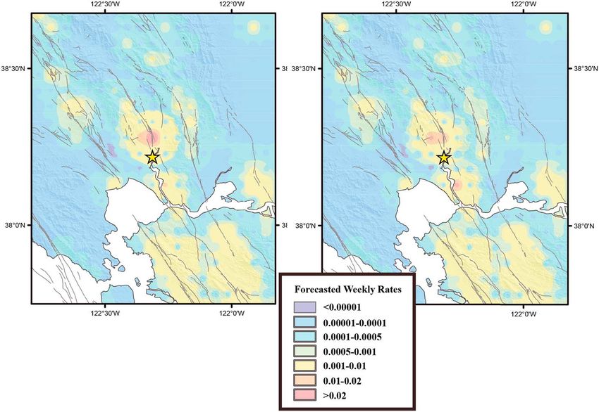
PUBLICATIONS
Geophysical Research Letters
RESEARCH LETTER                                 Stress-based aftershock forecasts made within 24 h
10.1002/2014GL062379
                                                postmain shock: Expected north San Francisco
Key Points:
• The West Napa earthquake changed
                                                Bay area seismicity changes after the 2014
  stress on Bay Area faults
• Rapid stress-based earthquake
                                                M=6.0 West Napa earthquake
  forecasts for evaluating methods              Tom Parsons1, Margaret Segou2, Volkan Sevilgen3, Kevin Milner4, Edward Field5, Shinji Toda6,
• Forecasts will be evaluated against the
  actual aftershock patterns                    and Ross S. Stein1
                                                1
                                                  U.S. Geological Survey, Menlo Park, California, USA, 2Geosciences Azur, Sophia Antipolis, France, 3Seismicity.net, San Carlos,
Supporting Information:                         California, USA, 4Southern California Earthquake Center, University of Southern California, Los Angeles, California, USA,
• Readme                                        5
                                                  U.S. Geological Survey, Golden, Colorado, USA, 6Tohoku University, Sendai, Japan
• Table S1

Correspondence to:                              Abstract We        calculate stress changes resulting from the M = 6.0 West Napa earthquake on north
T. Parsons,
tparsons@usgs.gov                               San Francisco Bay area faults. The earthquake ruptured within a series of long faults that pose
                                                significant hazard to the Bay area, and we are thus concerned with potential increases in the probability
                                                of a large earthquake through stress transfer. We conduct this exercise as a prospective test because
Citation:
Parsons, T., M. Segou, V. Sevilgen,             the skill of stress-based aftershock forecasting methodology is inconclusive. We apply three methods:
K. Milner, E. Field, S. Toda, and R. S. Stein   (1) generalized mapping of regional Coulomb stress change, (2) stress changes resolved on Uniform
(2014), Stress-based aftershock forecasts
                                                California Earthquake Rupture Forecast faults, and (3) a mapped rate/state aftershock forecast. All
made within 24 h postmain shock:
Expected north San Francisco Bay area           calculations were completed within 24 h after the main shock and were made without benefit of known
seismicity changes after the 2014 M = 6.0       aftershocks, which will be used to evaluative the prospective forecast. All methods suggest that we
West Napa earthquake, Geophys. Res.
                                                should expect heightened seismicity on parts of the southern Rodgers Creek, northern Hayward, and
Lett., 41, 8792–8799, doi:10.1002/
2014GL062379.                                   Green Valley faults.

Received 30 OCT 2014
Accepted 3 DEC 2014
Accepted article online 5 DEC 2014              1. Introduction
Published online 18 DEC 2014
                                                On 24 August 2014, the largest earthquake since the 1989 M = 7.0 Loma Prieta shock struck the San
                                                Francisco Bay area, the M = 6.0 West Napa event. This earthquake nucleated ~11 km beneath Napa Valley on
                                                or near the West Napa fault, which is itself one a series of subparallel right-lateral strike-slip faults that
                                                comprise the San Andreas fault system. The M = 6.0 earthquake injured 120 people, three critically, and
                                                caused localized damage in Napa Valley. The setting of this earthquake between the Hayward-Rodgers
                                                Creek system to the west and the Concord-Green Valley faults to the east (Figures 1 and 2) raises concerns
                                                that stress imparted by the West Napa earthquake might bring sections of these faults closer to failure,
                                                potentially triggering M > 7 events [e.g., Field et al., 2014]. We additionally want to test stress change
                                                forecasting prospectively by making calculations on the same day of the earthquake before seeing the
                                                spatial pattern of aftershocks. While there will be more refined information about the West Napa earthquake
                                                rupture available in the future, our goal is to attempt to forecast immediate seismicity effects on
                                                surrounding faults at a variety of scales. As there is uncertainty about the most effective approach in
                                                resolving calculated stress change onto fault targets, and how best to relate them to seismicity changes
                                                [e.g., Woessner et al., 2011], we try three different methods. We will revisit this prospective forecast in
                                                subsequent years to evaluate its performance based on subsequent seismicity, creep, and surface strain.
                                                We have produced stress-based forecasts following the 2005 M = 7.6 Kashmir and 2008 M = 7.9
                                                Wenchuan earthquakes [Parsons et al., 2006, 2008], subsequently evaluated their performance [Parsons
                                                et al., 2012], and then reevaluated after a large aftershock to the Wenchuan event occurred in 2013
                                                [Parsons and Segou, 2014].
                                                The initial submission of this publication was recorded on 3 September 2014; two of the forecasts produced
                                                here were not advised by any aftershocks, and the third used only the first 4 h to define the rupture plane.
                                                This revised publication makes use of aftershocks through 16 October 2014 to make very preliminary
                                                evaluations of the methods but not to change the forecasts.

PARSONS ET AL.                                                    ©2014. American Geophysical Union. All Rights Reserved.                                                 8792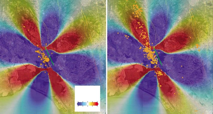
Geophysical Research Letters 10.1002/2014GL062379
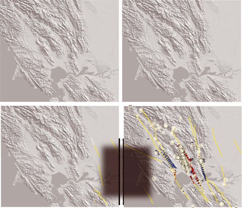
Figure 1. (a) Coulomb stress change surrounding the West Napa rupture; warm colors show calculated stress
(and therefore, hazard) increase, and cool colors show decreases (stress shadows). Based on the initial seismic moment
and initial 4 h of aftershocks, a 6 km × 6 km square source centered at 11 km depth with 1.3 m of slip was used to simulate
the M = 6.0 West Napa earthquake; the surface projection of the rupture surface is shown as the dashed red rectangle;
the rupture plane projects to the ground surface along the green line. The Northern California Seismic System (NCSS)
centroid moment tensor (CMT) solution with 155° strike, 82° dip, and 172° rake was used for the source. For simplicity, the
same geometry is assumed for all receiver faults, as they are predominantly vertical and right lateral, on which a friction
coefficient of μ = 0.4 was assumed at an 11 km depth. We calculate a ~0.25 bar stress increase on portions of the Green
Valley and Rodgers Creek faults, and a ~0.75 bar stress decrease along most of the West Napa fault. (b) Aftershocks through
16 October 2014 are plotted.
2. Methods
Three different methods for stress-based aftershock forecasting are applied independently by different
coauthors and completed within 24 h of the West Napa earthquake. All calculations are made with
preliminary information about the main shock rupture, namely, the Northern California Seismic System
(NCSS) centroid moment tensor (CMT) solution (http://www.ncedc.org/mt/nc72282711_MT.html), and could
be readily automated for operational earthquake forecasting. The three methods evolve from (1) mapping
spatial stress changes, (2) probability changes on mapped faults, and (3) an explicit, grid-based forecast
seismicity rate. A stress change map by itself suggests regions where enhanced or diminished seismicity
might be expected; however, many factors need to be accounted for, including magnitude of stress
change, normalizing seismicity density by relative areas of stress change, and also fault source density
(an area with many faults is likely to produce more earthquakes regardless of stress change). We therefore
explore fault-based and grid-based methods.
2.1. Coulomb Stress Change Mapping on Generalized Fault Planes
We calculate Coulomb stress change by simulating an earthquake with a slipping dislocation in an elastic
half-space [Okada, 1992; Toda et al., 1998; Stein, 1999] (Figure 1). Here a 6 km by 6 km square rupture source
with geometry taken from the NCSS CMT solution (155° strike, 82° dip, and 172° rake) with 1.3 m of slip centered
at the hypocenter 11 km deep conserves the M = 6.0 West Napa earthquake moment (1.3 × 1025 dyn cm).
The Coulomb criterion (ΔCFF) is defined by
ΔCFF ≡ jΔτ f j þ μ′ ðΔσ n ΔpÞ (1)
where Δτ f is the change in shear stress on the receiver fault (set positive in the direction of fault slip), μ is
the coefficient of friction, Δσ n is the change in normal stress acting on the target fault (set positive for
unclamping), and Δp is pore pressure change. The Coulomb stress change is resolved on receiver fault
planes that could have any geometry, rake, and friction. Here the receivers are assumed to have the same
characteristics as the rupture source, which is consistent with the regional northwest trending strike-slip
tectonics of the San Andreas fault system. The calculation in Figure 1 assumes a receiver fault friction
coefficient of μ = 0.4, depth of 11 km, and pore fluid effects are neglected.
PARSONS ET AL. ©2014. American Geophysical Union. All Rights Reserved. 8793Geophysical Research Letters 10.1002/2014GL062379
Figure 2. Coulomb stress change resolved on mapped faults defined by the Uniform California Earthquake Rupture
Forecast Version 3 (UCERF3). Red dots correspond to calculated stress increases, whereas blue dots correspond to
calculated decreases. Dots are located at centers of receiver fault patches (~3 km × 3 km); dipping faults are thus wider in
map view. (a–c) Regardless of friction coefficient used, we find that the Hayward-Rodgers Creek fault junction, the Franklin
fault, the Contra Costa shear zone, and the West Napa fault have calculated stress increases. (d) Aftershocks through 16
October 2014 are plotted, and the inset histogram shows the distribution of aftershocks associated (within ±3 km) with
fault planes that have calculated stress increases or decreases.
Stress change mapping provides an estimate of the time-independent, spatial distribution of future
seismicity. Therefore, the prediction is that aftershocks will preferentially occur in areas of calculated stress
increase and will be less likely in calculated stress-decreased areas. This can be readily tested against the
observed pattern of seismicity density at any time over the duration of aftershocks after accounting for
background rates and fault distribution [e.g., Parsons et al., 2012; Parsons and Segou, 2014].
2.2. Coulomb Stress Resolved on Mapped Fault Planes
An alternative approach to stress change calculation focuses on mapped faults. This technique is less
likely to capture the complete spatial pattern of aftershocks but appears to be effective at forecasting
higher magnitude earthquakes [Parsons et al., 2012]. We work with faults defined by the Uniform California
Earthquake Rupture Forecast Version 3 (UCERF3) [Dawson, 2013], which have geometries and rakes
determined through a geological consensus process, and have calculated long-term M > 5.5–6.0 rupture
rates [Field et al., 2014]. Receiver faults are divided into ~3 km by ~3 km patches, and Coulomb stress is
resolved on each (Figure 2). The receiver fault friction coefficient is almost impossible to know even in
detailed studies, so a range is used here from μ = 0.2 to μ = 0.8. We use the NCSS CMT solution parameters
for the main shock slip model modified slightly to match the UCERF3 geometry for the West Napa fault
(155° strike, 75° dip, and 180° rake). We centered the source dislocation at the initial reported hypocenter
depth of 10.7 km and scaled its dimensions using the regressions of Wells and Coppersmith [1994] for strike-slip
rupture length (16 km), width (7.7 km), and average slip (0.15 m) at depth for a M = 6.0 earthquake.
PARSONS ET AL. ©2014. American Geophysical Union. All Rights Reserved. 8794Geophysical Research Letters 10.1002/2014GL062379
We assess the impact of the West Napa earthquake by calculating earthquake probability changes on major
faults. A stress change can theoretically advance or delay earthquakes by time T′, which can be calculated
by dividing the stress change (ΔCFF) by the tectonic stressing rate (˙τ), as T ′ = Δτ/ τ̇. Time-dependent probability
calculations can be adjusted by accruing probability from the last earthquake time modified by the advance
or delay (T0 + Τ ′). Alternatively, the earthquake recurrence interval ξ can be adjusted by the clock change as
ξ = ξ 0 T ′. We use the latter approach since the last earthquake time is unknown for north Bay Area faults.
We use the central value of μ = 0.4 for calculating ΔCFF for probability changes since it is close to the average.
To explain Omori law transient earthquake rate changes with rate/state theory, Dieterich [1994] derived an
expression for time-dependent seismicity rate R(t), after a stress perturbation as
r
RðtÞ ¼ ΔCFF h i (2)
exp aσ 1 exp t ta þ 1
where r is the steady state seismicity rate, ΔCFF is the stress step, σ is the normal stress, a is a fault constitutive
constant, and ta is an observed or inferred aftershock duration. We assume ta to be 10 years and derive the aσ
parameter from aσ ¼ t a τ̇ [Dieterich, 1994], which yields values between 0.25 and 0.5 bars based on loading
rates from Parsons [2002] and is consistent with the 0.5 bar value of Toda et al. [2005].
The transient earthquake rate R(t) after a stress step can be related to earthquake probability over the interval
Δt as
tþΔt
Pðt; Δt Þ ¼ 1 exp ∫t Rðt Þdt ¼ 1 expðNðt ÞÞ; (3)
[Dieterich and Kilgore, 1996], where N(t) is the expected number of earthquakes in the interval. The transient
probability change can be superimposed on recurrence interval change. Integrating for N(t) yields
( " #)
1 þ exp ΔCFF 1 exp Δt
NðtÞ ¼ r p Δt þ ta ln aσ
t a
(4)
exp ΔCFF
aσ
where rp is the expected rate of earthquakes associated with the permanent probability change [Toda et al.,
1998]. This rate can be determined by applying a stationary Poisson probability expression as
1
rp ¼ lnð1 Pc Þ (5)
Δt
where Pc is a conditional probability and can be calculated using any distribution. The time-dependent
Brownian Passage Time (BPT) model is used here [Matthews et al., 2002], with a fixed aperiodicity of 0.5, and
recurrence intervals from Field et al. [2014]. No dates of past large earthquakes are known for north San
Francisco Bay region faults, so we use the method of Field and Jordan [2014] to account for unknown time of
last event before an historical open interval (tH = A.D. 1776 for the San Francisco Bay region, Working Group on
California Earthquake Probabilities [2003]) as
tH þΔt
Δt ∫tH F ðt Þdt
PðΔt jt > t H Þ ¼ ∞ ; (6)
∫t H
½1 F ðt Þdt
where F(t) is the probability density function (BPT in this case).
We can use this expression to calculate time-dependent probability for any duration; we give values for 1 and
5 year spans on each fault subsection (length equal to half downdip width) that has a stress change magnitude
≥0.1 bar (Table 1). Probabilities are for events equal to or greater than the minimum magnitude for which we have
rate information (M ~ 6). Evaluation of these calculations depends on an event of this magnitude occurring.
2.3. Coulomb and Rate/State Aftershock Forecasting
We lastly combine Coulomb stress changes and rate/state equations [Dieterich, 1994] to map expected
seismicity rates following the stress perturbation from the West Napa event. To model the evolution of
seismicity, we calculate Coulomb stress change on a 2.5 km by 2.5 km grid at target depth 10 km imparted by
the West Napa earthquake for optimally oriented planes (friction varying over μ = 0.2 to μ = 0.8), with a
regional stress field representation taken from Hardebeck and Michael [2004], with the maximum compressive
stress set to N19°E at a differential stress magnitude of σ1–σ3 = 10 MPa [Toda et al., 2005]. We make a second
PARSONS ET AL. ©2014. American Geophysical Union. All Rights Reserved. 8795Geophysical Research Letters 10.1002/2014GL062379
Table 1. Earthquake Probability Change Values Averaged Across UCERF3 Subsections; Values Are for M ≥ Mmin as Given
a
for Each Fault
One Year Probability (%) Five Year Probability (%)
M ≥ Mmin M ≥ Mmin
UCERF3 Fault Mmin ΔCFF (bar) BPT Interaction Δ BPT Interaction Δ
Bennett Valley 6.00 0.17 0.09 0.04 59 0.45 0.21 55
Bennett Valley + 6.00 0.13 0.09 0.15 64 0.46 0.68 48
Contra Costa Shear Zone (Connector) 6.22 0.12 0.06 0.12 89 0.31 0.51 65
Franklin 6.25 0.21 0.06 0.15 141 0.32 0.59 89
Green Valley 5.54 0.26 0.36 0.17 54 1.80 0.92 50
Green Valley + 5.76 0.15 0.43 0.76 77 2.13 3.39 59
North Hayward 6.04 0.10 0.34 0.28 18 1.68 1.43 15
North Hayward + 6.12 0.16 0.30 0.48 62 1.48 2.17 47
Hunting Creek-Berryessa 5.86 0.10 0.31 0.21 33 1.56 1.12 29
Rodgers Creek-Healdsburg 6.18 0.13 0.32 0.18 44 1.59 0.97 39
Rodgers Creek-Healdsburg + 6.17 0.13 0.30 0.50 65 1.52 2.27 49
West Napa 6.30 1.64 0.11 0.00 99 0.55 0.01 99
West Napa + 6.30 1.17 0.12 0.21 83 0.59 0.94 61
a
Average stress change values are given for each fault; most of the faults have significant areas of positive and negative
stress change (Figure 2), so the names are given with a “+” or “” symbol, respectively. “BPT” refers to time-dependent
probability using Brownian Passage Time distribution with no interactions, whereas “interaction” includes the recurrence
interval change and rate/state transient effects. “Δ” is the probability change factor, calculated as (Pinteraction PBPT )/PBPT.
calculation under an assumption that all receiver faults on the grid have properties akin to the Hayward fault
(strike = N34°W, dip = 90°, and rake = 180°) (Figures 3a and 3b). We include uncertainty in receiver fault
friction over a range of μ = 0.2 to μ = 0.8.
Under rate/state theory, a stress perturbation (ΔCFF) causes the state variable of the system γn 1 before the
event to evolve coseismically to a new value γn,
ΔCFF
γn ¼ γn1 exp (7)
aσ
Figure 3. (a) Forecast first week of M ≥ 3.0 seismicity rate density following the West Napa earthquake based on Coulomb
stresses calculated on a grid of optimally oriented planes (friction coefficient μ = 0.4) and (b) a grid of faults with Hayward
fault characteristics (strike = N34°W, dip = 90°, and rake = 180°).
PARSONS ET AL. ©2014. American Geophysical Union. All Rights Reserved. 8796Geophysical Research Letters 10.1002/2014GL062379
The forecast seismicity rate R is then found from
r
R¼ : (8)
γ τ̇
This model depends on three parameters: (1) the reference seismicity rate r (background seismicity rate),
which is taken from M ≥ 3.0 rates during a 1974–2014.235 period, (2) the mean secular fault loading rate on
all faults surrounding the rupture ( τ̇ = 0.05 bar/yr) [Parsons, 2002], and (3) the aσ term, taken to be 0.5 bar
after Toda et al. [2005]. We estimate expected M ≥ 3.0 seismicity at each node for the first week after the
main shock.
3. Results
3.1. Results From Coulomb Stress Change Mapping
The mapping in Figure 1 shows broad regions of calculated stress increases and decreases that affect major
fault zones north of San Francisco Bay. In particular, we calculate a ~0.25 bar stress increase on the southern
Rodgers Creek fault where it enters San Pablo Bay and steps west onto the northern Hayward fault.
Additionally, portions of the Green Valley fault also are calculated to have a ~0.25 bar increase; the Green
Valley fault is the northern extent of the potentially linked Concord fault system that runs east of the San
Francisco Bay area. We calculate a ~0.75 bar stress decrease on most of the West Napa fault.
At the time of the calculations we wrote in the initial draft of this paper: “The simplified rupture model we
used for the 2014 M = 6.0 West Napa earthquake means that we are unlikely to capture near-source
aftershock activity very accurately, and this map should instead be interpreted for expected activity on
adjacent faults.” This is shown by the aftershock pattern as of 16 October 2014 (Figure 1b), where many
near-source aftershocks are located in the stress-reduced area around the main shock, whereas more distant
events occur primarily in the stress-increased lobes.
3.2. Results From Coulomb Stress Changes Resolved on UCERF3 Faults
The spatial pattern of Coulomb stress changes resolved on individual faults in Figure 2 is comparable to the
generalized mapping in Figure 1 because most of the major faults are parallel to the West Napa earthquake
source. In this case we used a larger area source model with an order-of-magnitude lower average slip,
meaning that we calculate stress changes over a broader spatial extent, but with lower magnitudes in most
places (Figure 2). We do note some additional effects; most importantly for hazard implications, we calculate
a ~0.2 bar stress increase on the northern part of the Hayward fault, and a ~0.1 bar increase on the southern
Rodgers Creek fault. We find a ~0.2 bar increase on parts of the Franklin and Green Valley faults, and a
~0.1 bar increase on the Contra Costa shear zone. Strong stress increases and decreases (between 1 and
2 bar) are calculated on the West Napa fault, though uncertainty about the exact location of the main shock
rupture affects near-source stress calculations. We find that if we associate aftershocks with fault surfaces
(defined as being ±3 km from 3-D fault plane), then 127 aftershocks that occurred through 16 October 2014
are associated with calculated stress increases versus 24 that are associated with stress decreases (Figure 2d).
Annual and 5 year time-dependent (BPT) probability calculations are made for each fault subsection with and
without stress interaction from the West Napa event. Annual probability is generally low (< 1%) and not
significantly different than Poisson because of the short duration, but is strongly affected (~10–50% changes)
by stress changes (Table 1). Values are given for every subsection in the supporting information. We
suggest that these probability values are best utilized in a relative sense because the probability of a M ~ 6
earthquake striking over a 1–5 year period are always low in the Bay Area; given that the Green Valley,
North Hayward, and south Rodgers Creek faults would be considered the most dangerous in the aftermath
of the West Napa earthquake.
3.3. Results From Coulomb/Rate-State Aftershock Forecasting
We make direct M ≥ 3.0 aftershock forecasts based on Coulomb stress change mapping in Figure 3. The
two calculations based on optimal versus regionally aligned receiver faults are similar enough to discuss
concurrently. We calculate that the highest expected weekly rate (≥0.02) of M ≥ 3.0 earthquakes will be on the
Green Valley fault northeast of the rupture zone (Figure 3). We also calculate relatively lower but increased
M ≥ 3.0 rates above background (up to 0.01/week) on the Hayward, Rodgers Creek, and Bennett Valley faults.
PARSONS ET AL. ©2014. American Geophysical Union. All Rights Reserved. 8797Geophysical Research Letters 10.1002/2014GL062379
Rates calculated from stress-based methods tend to underpredict compared with observed values during the
earliest phases of the aftershock period, primarily because reference background rates tend to be low, as the
observation periods are not long enough to be fully representative [e.g., Segou et al., 2013].
We evaluate the performance of the models using log-likelihood statistics [Schorlemmer et al., 2007], and we
find that the models underestimate the number of observed events with δ1 = 3.03 × 10 6, and δ2 ≅ 1, and
they are rejected within the first week. The spatial performance of the models is similar with small differences
in joint log likelihood, δjLLH = 0.0038 and average LLH value of 0.32. However, a preliminary retrospective
parameter optimization procedure, often used in statistical forecasting [e.g., Werner et al., 2011], reveals
that a stressing rate for the Napa Fault of ~0.005 bar/yr leads to a successful performance evaluation. This
implies that a short learning period might enable better forecast results.
4. Conclusions
We forecast future seismicity from three stress-based methods for short (1 week) to intermediate (1–5 years)
using information available within the first 24 h after a main shock. The purpose is to evaluate whether rapid,
physics-based methods should have any role in operational forecasts. All three methods lead to similar
conclusions. Earthquake rate increases are likely on parts of the Green Valley, Franklin, Contra Costa, southern
Rodgers Creek, and northern Hayward faults as a result of the 24 August 2014 M = 6.0 West Napa earthquake.
Earthquake rate decreases are also expected on parts of the Bennett Valley, Green Valley, Hayward, and
Rodgers Creek faults. Initial results suggest that stress changes are consistent with the spatial pattern of
aftershocks, though a spatial rate/state forecast was rejected within the first week, and requires a learning
period to adjust stressing rate parameters. We will evaluate the longer-term forecasts using observed
seismicity rate changes, creep, and surface strain.
Acknowledgments References
We accessed the event page for the
Dawson, T. E. (2013), Appendix A—Updates to the California reference fault parameter database—Uniform California Earthquake Rupture
24 August 2014 M = 6.0 West Napa
Forecast, version 3 fault models 3.1 and 3.2, U.S. Geol. Surv. Open File Rep., 2013–1165, 66 pp. [Available at http://pubs.usgs.gov/of/2013/
earthquake at http://earthquake.usgs.
1165/pdf/ofr2013-1165_appendixA.pdf.]
gov/earthquakes/eventpage/
Dieterich, J. (1994), A constitutive law for rate of earthquake production and its application to earthquake clustering, J. Geophys. Res., 99,
nc72282711#scientific for rapid CMT
2601–2618, doi:10.1029/93JB02581.
information from NCSS. We thank
Dieterich, J. H., and B. Kilgore (1996), Implications of fault constitutive properties for earthquake prediction, Proc. Natl. Acad. Sci. U.S.A., 93,
Editor Andrew Newman and two
3787–3794.
anonymous reviewers.
Field, E. H., and T. H. Jordan (2014), Time-dependent renewal-model probabilities when date of last earthquake is unknown, Bull. Seismol. Soc.
Am., in press.
The Editor thanks John McCloskey and
Field, E. H., et al. (2014), Uniform California Earthquake Rupture Forecast, version 3 (UCERF3)—The time-independent model, Bull. Seismol.
an anonymous reviewer for their
Soc. Am., 104, 1122–1180, doi:10.1785/0120130164.
assistance in evaluating this paper.
Hardebeck, J. L., and A. J. Michael (2004), Stress orientations at intermediate angles to the San Andreas fault, California, J. Geophys. Res., 109,
B11303, doi:10.1029/2004JB003239.
Matthews, M. V., W. L. Ellsworth, and P. A. Reasenberg (2002), A Brownian model for recurrent earthquakes, Bull. Seismol. Soc. Am., 92,
2233–2250.
Okada, Y. (1992), Internal deformation due to shear and tensile faults in a half-space, Bull. Seismol. Soc. Am., 82, 1018–1040.
Parsons, T. (2002), Post-1906 stress recovery of the San Andreas fault system from 3-D finite element analysis, J. Geophys. Res., 107(B8), 2162,
doi:10.1029/2001JB001051.
Parsons, T., and M. Segou (2014), Stress, distance, magnitude, and clustering influences on the success or failure of an aftershock forecast:
The 2013 M = 6.6 Lushan earthquake and other examples, Seismol. Res. Lett., 85, 44–51, doi:10.1785/0220130100.
Parsons, T., R. S. Yeats, Y. Yagi, and A. Hussain (2006), Static stress change from the 8 October, 2005 M = 7.6 Kashmir earthquake, Geophys. Res.
Lett., 33, L06304, doi:10.1029/2005GL025429.
Parsons, T., C. Ji, and E. Kirby (2008), Stress changes from the 2008 Wenchuan earthquake and increased hazard in the Sichuan basin, Nature,
454, 509–510, doi:10.1038/nature07177.
Parsons, T., Y. Ogata, J. Zhuang, and E. L. Geist (2012), Evaluation of static stress change forecasting with prospective and blind tests, Geophys.
J. Int., 188, 1425–1440, doi:10.1111/j.1365-246X.2011.05343.x.
Schorlemmer, D., M. C. Gerstenberger, S. Wiemer, D. D. Jackson, and D. A. Rhoades (2007), Earthquake likelihood model testing, Seismol. Res.
Lett., 78(1), 17–29, doi:10.1785/gssrl.78.1.17.
Segou, M., T. Parsons, and W. Ellsworth (2013), Evaluation of combined physics based and statistical forecast models, J. Geophys. Res. Solid
Earth, 118, 6219–6240, doi:10.1002/2013JB010313.
Stein, R. S. (1999), The role of stress transfer in earthquake occurrence, Nature, 402, 605–609.
Toda, S., R. S. Stein, P. A. Reasenberg, J. H. Dieterich, and A. Yoshida (1998), Stress transferred by the 1995 Mw = 6.9 Kobe, Japan, shock: Effect
on aftershocks and future earthquake probabilities, J. Geophys. Res., 103, 24,543–24,565, doi:10.1029/98JB00765.
Toda, S., R. S. Stein, K. Richards-Dinger, and S. Bozkurt (2005), Forecasting the evolution of seismicity in southern California: Animations built
on earthquake stress transfer, J. Geophys. Res., 110, B05S16, doi:10.1029/2004JB003415.
Wells, D. L., and K. J. Coppersmith (1994), New empirical relationships among magnitude, rupture length, rupture width, rupture area, and
surface displacement, Bull. Seismol. Soc. Am., 84, 974–1002.
PARSONS ET AL. ©2014. American Geophysical Union. All Rights Reserved. 8798Geophysical Research Letters 10.1002/2014GL062379
Werner, M. J., A. Helmstetter, D. D. Jackson, and Y. Y. Kagan (2011), High-resolution long-term and short-term earthquake forecasts for
California, Bull. Seismol. Soc. Am., 101, 1630–1648.
Woessner, J., S. Hainzl, W. Marzocchi, M. J. Werner, A. M. Lombardi, F. Catalli, B. Enescu, M. Cocco, M. C. Gerstenberger, and S. Wiemer (2011),
A retrospective comparative forecast test on the 1992 Landers sequence, J. Geophys. Res., 116, B05305, doi:10.1029/2010JB007846.
Working Group on California Earthquake Probabilities (2003), Earthquake probabilities in the San Francisco Bay region: 2002–2031, U.S. Geol.
Surv. Open File Rep., 03-214, 235 pp.
PARSONS ET AL. ©2014. American Geophysical Union. All Rights Reserved. 8799You can also read