Spatial and Social Frictions in the City: Evidence from Yelp
←
→
Page content transcription
If your browser does not render page correctly, please read the page content below
Spatial and Social Frictions in the City:
                          Evidence from Yelp∗
           Donald R. Davis†                   Jonathan I. Dingel‡               Joan Monras§
         Columbia and NBER                      Chicago Booth                    Sciences Po
                                        Eduardo Morales¶
                                      Princeton and NBER
                                         October 2015
                                  Preliminary and Incomplete

                                                Abstract
           We employ user-generated data from the website Yelp.com to estimate how spatial
       and social frictions combine to shape consumption choices within cities. Travel time,
       from both home and work, plays a first-order role in consumption choices. Users
       are two to four times more likely to visit a venue that is half as far away. Social
       frictions also play a large role. Individuals are less likely to visit venues in places
       demographically different from their own neighborhood. A one-standard-deviation
       increase in demographic distance is equivalent to a 21% increase in travel time in
       terms of reduced visits. Higher crime rates reduce visit probabilities. Women are
       about 50% more responsive than men to local robbery rates.

   ∗
     We thank Treb Allen, David Atkin, Victor Couture, Ingrid Gould Ellen, Mogens Fosgerau, Marcal
Garolera, Joshua Gottlieb, Jessie Handbury, Albert Saiz, and seminar audiences at the NBER Summer
Institute URB meeting, Urban Economics Association, NBER Fall ITI meeting, Princeton, NYU Stern,
Duke ERID spatial-equilibrium conference, University of Barcelona - IEB, Yale, the Université du Québec à
Montréal, Toronto, and UCLA for helpful comments. We thank Bowen Bao, Luis Costa, David Henriquez,
Charlene Lee, Ludwig Suarez, and especially Ben Eckersley, Hadi Elzayn, and Benjamin Lee for research
assistance. Thanks to the New York Police Department, and especially Gabriel Paez, for sharing geo-
coded crime data. Dingel thanks the Kathryn and Grant Swick Faculty Research Fund at the University of
Chicago Booth School of Business for supporting this work. Monras thanks the Banque de France Sciences
Po partnership and LIEPP for financial support. Part of this work is supported by a public grant overseen
by the French National Research Agency (ANR) as part of the “Investissements d’Avenir” program LIEPP
(ANR-11-LABX-0091, ANR-11-IDEX-0005-02).
   †
     drdavis@columbia.edu
   ‡
     jdingel@chicagobooth.edu
   §
     joan.monras@sciencespo.fr
   ¶
     ecmorale@princeton.edu

                                                     1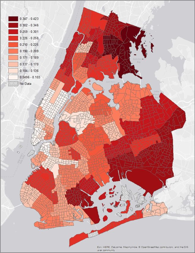
1    Introduction
Cities make us more productive, but they also provide attractive consumption opportunities
(Glaeser, Kolko, and Saiz, 2001). Consumption in cities often requires travel, so the value
of these consumption opportunities depends on the geography of the city (Couture, 2014).
Home and work are our primary locations within the city. And so home, work, and the
commute between the two are the primary bases from which our consumption is launched.
    Consumers’ decisions in cities are influenced by both the products offered and other
features of the urban context. We use the term “friction” to refer to determinants of demand
beyond products’ characteristics and prices. These frictions, which can be understood as
components of a broader set of product characteristics, depend on both the location of the
product and the identity of the consumer. Spatial frictions are costs of traversing the city
that influence consumer decisions by making consumption farther away less attractive. These
frictions play a central role in theories of spatial competition, dating to Hotelling (1929).
    Spatial frictions fragment the city, making it less valuable to consumers. But frictions
are not only spatial, they are also social. Social frictions are demographic or socioeconomic
characteristics of locations that influence individuals’ decisions to consume there. If aversion
to differences in ethnicity, race, or income reduces our willingness to take advantage of
consumption opportunities, then the value of the city is diminished. Concerns over perceived
safety, which often relate to such differences, may also shape consumer decisions. These social
frictions need not affect all members of society similarly; they could vary by ethnicity, race,
or gender.
    In this paper, we explore empirically how spatial and social frictions govern our use of the
city. Our work characterizes the consumption decisions of individuals living in New York City
who use Yelp.com, a website where users review local businesses. The data we collected from
Yelp users’ reviews identify their home and work locations and businesses patronized. We
combine this information with data on places within New York City. The resulting dataset
is novel in that it captures four dimensions necessary to studying consumption within the
city. It identifies the restaurants patronized by consumers, characteristics of restaurants
both chosen and unchosen, mode-specific travel times from users’ home and work locations
to these restaurants, and measures of social frictions within New York City.
    We characterize consumer preferences by estimating a discrete-choice model of restaurant-
visit decisions. Our estimates show that both spatial and social frictions influence the geog-
raphy of consumption. First, we quantify the role of spatial frictions for consumption within
the city. We estimate consumers’ aversion to incurring longer travel times, controlling for
product characteristics like restaurants’ ratings and prices. Our model specification accounts
for the facts that consumption may originate at home, work, or the commute between them
and that both automobile and public transit are possible modes of transport. Across origin-
mode pairs, halving the minutes of travel time to a venue would imply that the user would
be two to nearly four times more likely to visit the venue from that origin by that mode.
These are important parameters for quantitative assessments of consumption in the city,
such as Allen, Arkolakis, and Li (2015). Further, our estimates imply that models of urban
consumption are misspecified if they omit visits originating from the workplace.
    Second, we quantify the role of demographic differences in consumers’ decisions and find
that this social friction plays an important role. Ceteris paribus, a user would be 27% more

                                               2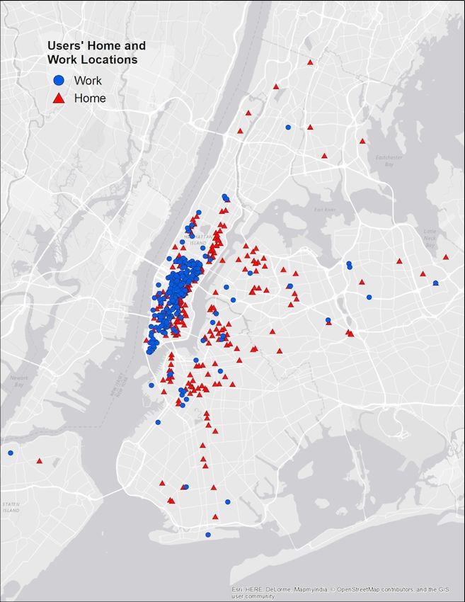
likely to visit a venue in a census tract that is one standard deviation more demographically
similar to her home tract. Moreover, these frictions are not symmetric. While users on
average are less likely to visit a census tract that has demographics different from those of
their own residence, the negative effect of demographic differences is more than twice as
large when the destination tract is plurality black. Finally, beyond tract-level demographic
differences, the racial/ethnic identity of individual users predicts their consumption behavior.
Our estimates demonstrate homophily with regard to the user’s race/ethnicity, implying that
socioeconomic shifts such as gentrification have heterogeneous consequences for residents as a
function of their identities. The finding that demographic differences deter visits implies that
economic interactions are even more segregated than would be predicted by the combination
of residential segregation and spatial frictions.
    Third, we find a significant gender differential in the incidence of crime. Users are less
likely to visit venues in places where more robberies occur, and women are significantly less
likely than men to visit venues in neighborhoods with more robberies. These effects are
modest in magnitude given the low levels of robberies in contemporary New York City, but
they imply that the substantial decline in crime in New York City over the last twenty-
five years was particularly advantageous to females, since females’ use of the city is more
responsive to crime rates.
    Our findings relate to several strands of literature. First, we study the geography of
consumption within the city. A recent literature has documented cross-city variation in
the tradable goods available for consumption (Handbury and Weinstein, 2011; Handbury,
2012), and geographic variation in non-tradables has been posited to shape the relative at-
tractiveness of cities (Glaeser, Kolko, and Saiz, 2001). This dimension of economic life has
grown increasingly important in recent decades.1 Prior studies of the geography of con-
sumption within the city include Couture (2014), who infers the benefits of variety due to
urban density from the time individuals spend traveling from their homes to restaurants,
Houde (2012), who demonstrates that a demand model incorporating potential consumers’
commuting paths better matches observed sales than a model estimated under the assump-
tion that all consumer trips originate at their home locations, Katz (2007), who studies the
impact that driving time from home has on the choice of grocery stores by consumers, and
Eizenberg, Lach, and Yiftach (2015), who estimate within-city travel costs for consumers
using data on neighborhood-level expenditure shares for Jerusalem supermarkets. Relative
to this prior work, we exploit data describing individuals’ home and work locations, their
demographics, and characteristics of the venues they patronize. This allows us to estimate
the effect of spatial frictions on consumer decisions while accounting for product character-
istics. Furthermore, while prior literature has focused on spatial frictions, we emphasize the
role of social frictions in shaping consumption within cities.
    Our paper is also related to a large literature on social and economic fragmentation
related to demographic differences. Much of that literature has documented ethnic and
racial fragmentation in terms of residential segregation (Cutler, Glaeser, and Vigdor, 1999;
   1
    US households’ share of food spending devoted to food prepared away from home grew from less than
26% in 1970 to more than 43% in 2012. While the number of daily commuting trips has stayed relatively
steady for decades, trips for social/recreational purposes have steadily grown (Commuting in America III,
2006).

                                                   3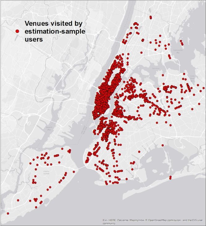
Echenique and Fryer, 2007; Bayer and McMillan, 2008).2 Many US cities are de facto quite
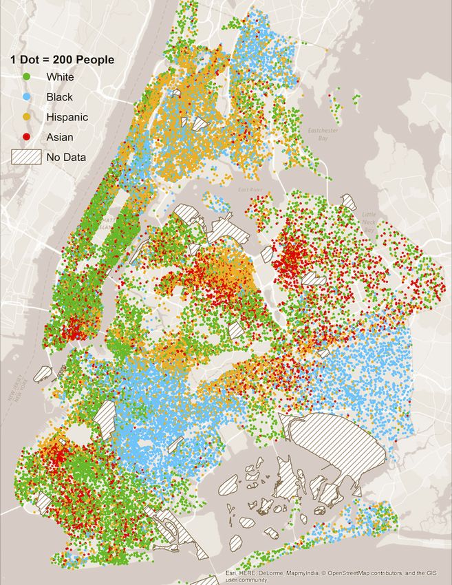
segregated. Figure 1 depicts the population of New York City using colored dots to repre-
sent people of four different demographic groups – whites (green), blacks (blue), Hispanics
(orange), and Asians (red).3 There is a clear pattern of residential segregation. Some of
the mechanisms posited to explain residential segregation would also predict segregation in
individuals’ consumption patterns. For example, between countries, lower bilateral trust
reduces trade and investment (Guiso, Sapienza, and Zingales, 2009), and closer cultural ties
can facilitate economic exchange (Rauch, 2001). A number of studies have documented
retail-shopping frictions related to racial/ethnic composition (Lee, 2000; Ayres, 2001; An-
tecol and Cobb-Clark, 2008; Schreer, Smith, and Thomas, 2009). This paper quantifies how
demographic differences shape which places people visit for consumption purposes. We use
information on the demographic composition of residents surrounding venues and users’ res-
idential locations, as well as the ethnicity or race of the user, to demonstrate that ethnic or
racial dissimilarity reduces economic interactions within New York City after accounting for
geography, venue characteristics, and income differences.
Third, while we know that crime affects local population size (Cullen and Levitt, 1999)
and local housing prices (Gibbons, 2004; Linden and Rockoff, 2008; Pope, 2008), there is
little evidence on the response of consumers to spatial variation in crime rates.4 Crime
rates, fear of crime, and residential segregation are interrelated phenomena (O’Flaherty and
Sethi, 2007, 2010). Specifically, the fraction of a neighborhood’s population that is black is
significantly associated with its residents’ perception of a crime problem, even after control-
ling for neighborhood crime rates (Quillian and Pager, 2001), and white survey respondents
more strongly associate racial composition with perceived risk (Quillian and Pager, 2010).
Our data on consumer choices allow us to separately study the influences of ethnic and
racial composition and criminal activity on the decisions of non-residents to patronize vari-
ous neighborhoods. Our estimates demonstrate a cost of crime beyond its immediate effects
on victims and residents in terms of diminishing the consumption value of the city for the
broader population.
Finally, our results are also related to previous research on the interaction between gender
and fear of crime (Doran and Burgess, 2011). A large majority of this literature is based on
surveys such as the General Social Survey and the National Crime Survey (Ferraro, 1996).
These studies uniformly find that fear of crime is higher among women (Pain (1991, p.416)).
The surveys also indicate that a very large fraction of women adjust their behavior in regard
to these fears, avoiding risky areas in ways that affect their social and leisure activities
(Pain, 1997; Lorenc, Clayton, Neary, Whitehead, Petticrew, Thomson, Cummins, Sowden,
and Renton, 2012). Our study complements these survey studies by using evidence coming
2
Echenique and Fryer (2007) have also studied how race affects students’ friendship networks within
schools.
3
This map was inspired by a New York Times project, “Mapping America: Every City, Every Block.”
4
There are consumer technologies devoted to this purpose. GPS devicemakers have developed technolo-
gies to incorporate crime statistics and demographic information when giving users navigational directions.
Microsoft patented incorporating crime statistics into route calculation so as to direct the user “through
neighborhoods with violent crime statistics below a certain threshold”. A Manhattan-based smartphone
app called “SketchFactor” crowdsourced opinions about the “sketchiness” of neighborhoods. The app came
under criticism for being racist and is now defunct (New Yorker, July 29, 2015).
4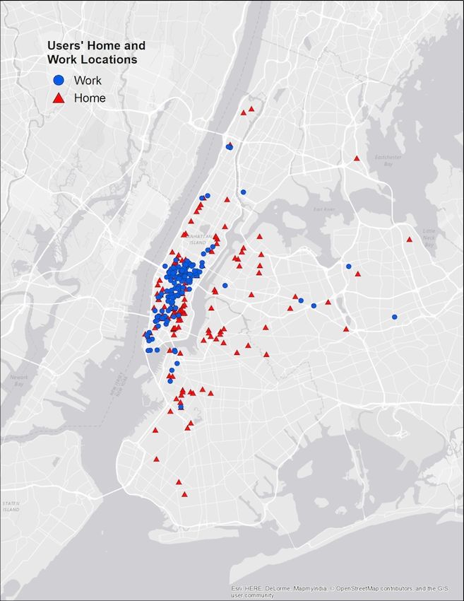
Figure 1: New York City population by race/ethnicity, 2010

Notes: This figure depicts the residential NYC population in terms of four
demographic categories that cover 97% of the population. Each dot represents
200 people. Tract-level population data from the 2010 Census of Population.

                                      5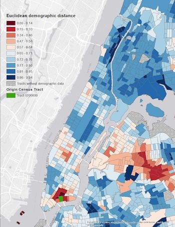
from actual consumption patterns of individuals. Additionally, a major advantage of our
data is that we have information describing the venues under consideration, allowing us to
control for these other determinants of demand when inferring how male and female users
respond. We find that female users are particularly sensitive to spatial variation in crime
rates.
    The remainder of this paper proceeds as follows. Section 2 introduces the data and
section 3 our empirical methodology. Section 4 reports our estimates of the roles of spatial
and social frictions in the city.

2       Data
We combine data from individual Yelp users with information on New York City to describe
how these individuals use the city.

2.1     Yelp data
Yelp.com is a website where users review local businesses, primarily restaurants and retail
stores (Yelp, 2013). The website describes a venue in terms of its address, hours of operation,
average rating, user reviews, and a wide variety of other characteristics. Yelp’s coverage of
restaurants is close to comprehensive (see appendix section A.4). The website is relevant
for the general population of restaurant consumers, as discontinuities in Yelp ratings have
been shown to have substantive effects on restaurants’ revenues (Luca, 2011) and reservation
availability (Anderson and Magruder, 2012).
    In addition to assigning a rating of one to five stars, users are encouraged to write
reviews describing their personal experience with a business. These reviews vary greatly
both in tone and length, ranging from a few sentences to many paragraphs. Crucial for our
purposes is that users often disclose information in their reviews about their residential and
work locations.5 This provides us a novel description of the links between the consumption
choices of individuals and a rich set of location- and venue-specific characteristics.
    We examined Yelp users’ reviews to identify their home and work locations. In mid-2011,
we gathered data from the Yelp website for users who had reviewed venues in New York City.
As described in detail in appendix A.3, we identified users’ residential and work locations
based on the text of reviews that contained at least one of 26 key phrases related to location,
such as “close to me,” “block away,” and “my apartment.” We classified whether the venue
under review was proximate to the user’s home and/or work locations. Using the set of
venues associated with users’ residential and work locations, we estimated the residential
and work locations using the average of the relevant venues’ latitude-longitude coordinates.
Restricting our sample to users who do not reveal a change in residence or workplace within
New York City and whose home and work locations can be assigned to census tracts with
no missing covariates yielded an estimation sample containing 406 users who wrote 16,573
    5
    Another example of using the information disclosed in reviews is searching Yelp to detect outbreaks of
food poisoning unreported to NYC health authorities (Harrison, Jorder, Stern, Stavinsky, Reddy, Hanson,
Waechter, Lowe, Gravano, and Balter, 2014).

                                                    6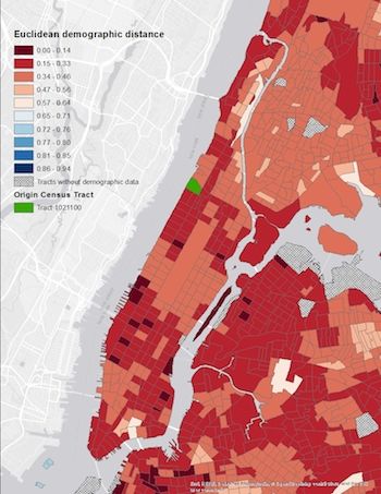
Figure 2: Locations of Yelp users in estimation sample

             Notes: This figure depicts the distribution of home and work locations of the
             406 users in our estimation sample.

reviews.6
    Figure 2 depicts the home and work locations of the users in our estimation sample. Con-
sistent with broader patterns, our identified users have a high concentration of employment
in Manhattan below 59th Street and a more dispersed residential pattern.
    Yelp users may also post information about themselves to their profile, such as a photo.
In some estimation exercises, we use a user’s apparent gender and ethnicity or race, inferred
from their user photo, to examine how consumer behavior depends on the interaction of user
characteristics and venue characteristics.7 A previous study compared such observational
measures of ethnicity and race inferred from photos with administrative data and found a
high degree of accuracy in partitioning subjects into three groups: Asian, black, and white
or Hispanic (Mayer and Puller, 2008).
    Table 1 reports summary statistics for these users’ gender, demographic, and locational
information. Females constitute more than 60% of the users in our estimation sample.8
Very few users were identified as blacks. Asians are overrepresented relative to their share
of the general population, as they constitute about one-third of our identifiable users but
only about 12% of New York City. The users in our estimation sample tend to live in census
   6
      If we omit work locations and use only home locations, there are more than 1800 users with nearly
40,000 reviews meeting these criteria. See appendix C.2 for a discussion of how our results are altered if we
fail to incorporate the workplace and commuting origins.
    7
      While users may choose “male” or “female” for their gender on their Yelp profile, this information is not
publicly displayed on their profile. All our empirical results describing differences between men and women
in fact describe differences between users who were classified based on their gender presentation in their
profile photo. Some profile photos do not present a gender (e.g. cartoon graphics, photos of animals).
    8
      Users with profile photos for which we could not classify the gender have both male and female dummy
variables equal to zero.

                                                      7
Table 1: User summary statistics
Variable Mean Std. Dev.
Number of restaurant reviews in estimation sample 40.95 42
User appears female in profile photo 0.61 0.49
User appears male in profile photo 0.34 0.47
User appears white or Hispanic in profile photo 0.44 0.5
User appears Asian in profile photo 0.26 0.44
User appears black in profile photo 0.03 0.16
User race/ethnicity indeterminate in profile photo 0.27 0.45
Median household income of home census tract (thousands dollars) 77.07 33.19
Share of home census tract population that is age 21-39 0.43 0.11
Notes: This table describes the 406 Yelp users in our estimation sample. Census tract
income data from 2007-2011 American Community Survey and demographic data from
2010 Census of Population.
tracts with median incomes typical of Manhattan but higher than typical of New York City
as a whole. The average of tract median household income in our estimation sample is near
$77,000, while the city-wide mean is about $56,000. The users in our estimation sample tend
to live in census tracts with a share of the population between the ages of 21 and 39 (43%)
that is higher than both Manhattan (37%) and New York City as a whole (30%). These
patterns are consistent with statements that Yelp’s global user base tends to be younger,
higher-income, and more educated than the population as a whole (Yelp, 2013).
The 406 users in our estimation sample posted more than 16,000 reviews of NYC restau-
rants between 1 January 2005 and 14 June 2011. Figure 3 displays all the restaurants
reviewed by the users in our estimation sample. Unsurprisingly, these venues are heavily
concentrated in lower Manhattan, but users in our estimation sample have reviewed venues
in many parts of New York City.
Table 2 summarizes the distribution of reviews in terms of venues’ prices, ratings, and
boroughs. The first two columns describe the estimation sample in terms of the number and
share of reviews. The third column reports these frequencies for all reviews of NYC Yelp
restaurants in our data, constituting more than 700,000 reviews. Comparing the second and
third columns of Table 2 shows that users in our estimation sample exhibit review frequencies
similar to that of the broader Yelp population. The frequencies of reviews across restaurants’
prices and ratings are very similar in columns two and three. This is consistent with the
hypothesis that users whose residences and workplaces we located based on the text of their
reviews are similar to the broader population of Yelp users in their restaurant-going behavior.
Users in our estimation sample review Manhattan venues slightly more than the population
of Yelp as a whole.
Figure 4 maps these data for two individuals in our estimation sample. In each panel,
red dots denote Yelp venues reviewed by this user. The “H” denotes the average coordinates
of those venues identified as residential locations in the text of this user’s reviews. The “W”
denotes the similarly defined work location. The user in the left panel lives and works in
midtown Manhattan. The other user works in midtown Manhattan and resides in a south-
eastern Manhattan development called Stuyvesant Town. At a glance, the maps suggests
8Figure 3: Restaurants reviewed by users in estimation sample
Notes: This map depicts the locations of 4993 Yelp restaurant venues reviewed
by users in our estimation sample. Each dot represents a venue.
9Table 2: Venue review summary statistics
Estimation sample Share of
Restaurant characteristic Observations Share of reviews all Yelp reviews
Price of $ 3875 .233 .228
Price of $$ 9345 .562 .566
Price of $$$ 2745 .165 .161
Price of $$$$ 659 .040 .045
Rating of 1 stars 9 .001 .001
Rating of 1.5 stars 32 .002 .002
Rating of 2 stars 120 .007 .011
Rating of 2.5 stars 590 .035 .038
Rating of 3 stars 2321 .140 .140
Rating of 3.5 stars 6202 .373 .359
Rating of 4 stars 6499 .391 .390
Rating of 4.5 stars 834 .050 .056
Rating of 5 stars 17 .001 .003
Located in Manhattan 13646 .821 .749
Located in Brooklyn 1862 .112 .169
Located in Queens 1003 .060 .069
Located in Bronx 52 .003 .008
Located in Staten Island 61 .004 .005
Notes: This table summarizes the distribution of reviews across different venue
characteristics in both our estimation sample (columns 1 and 2) and all Yelp users as
a whole (column 3). Comparing columns 2 and 3 shows that the review behavior of
users in our estimation sample is similar to that of Yelp users as a whole.
10Figure 4: Two users’ locations and restaurant reviews
Notes: These two maps display two users’ home and work locations and Yelp
restaurant venues reviewed.
that both proximity and venue characteristics influence user behavior. Both users primarily
review venues that are near their home or work locations. Both users visit more downtown
venues than uptown venues, which may reflect differences in the quantity or quality of venues
in these areas.
2.2 NYC crime, demographic, and transportation data
We combine the information from Yelp users’ reviews with data describing locations’ resi-
dential racial or ethnic composition, income levels, crime rates, and estimates of the time
required to travel between locations.
Much of the demographic and income information is reported at the level of census
tracts. Census tracts are geographic units defined by the US Census Bureau based on popu-
lation. We use data from the 2010 Census of Population to describe each tract’s residential
racial/ethnic composition in terms of Asians, blacks, Hispanics, and whites.9 These popula-
tion counts are depicted in Figure 1. The data on median household incomes come from the
2007-2011 American Community Survey 5-Year Estimate. These tract-level characteristics
9
To be precise, we divide the population into five racial/ethnic groups and use the population counts of
non-Hispanic whites, non-Hispanic blacks, non-Hispanic Asians, and all Hispanics. The remainder, which in-
cludes Native Americans, Hawaiians, other races, and mixed-race categories, constitutes about three percent
of the NYC population.
11Table 3: Tract-level summary statistics
Manhattan New York City
Variable Mean Std. Dev. Mean Std. Dev.
Population 5677 2993 3866 2115
Land area (square kilometers) 0.182 0.092 0.324 0.516
Median household income (thousands dollars) 76.339 44.344 56.292 27.152
Share of tract population that is Asian 0.117 0.129 0.125 0.154
Share of tract population that is black 0.142 0.195 0.245 0.297
Share of tract population that is Hispanic 0.232 0.228 0.265 0.222
Share of tract population that is white 0.484 0.302 0.335 0.31
Male share of census tract population 0.475 0.039 0.476 0.032
Share of census tract population that is age 21-39 0.374 0.117 0.302 0.084
Spectral segregation index for tract’s plurality 0.171 0.354 0.914 2.394
Average annual robberies per resident in tract, 2007-2011 0.005 0.015 0.003 0.009
Tract is plurality Asian 0.032 0.177 0.082 0.274
Tract is plurality black 0.125 0.332 0.251 0.434
Tract is plurality Hispanic 0.215 0.412 0.246 0.431
Tract is plurality white 0.627 0.484 0.421 0.494
Number of observations 279 2110
Notes: This table describes 2010 NYC census tracts for which an estimate of median
household income is available. Data on incomes from 2007-2011 American Community
Survey, demographics from 2010 Census of Population, robberies from NYPD.
are summarized in Table 3.
To describe crime rates, we computed tract-level robbery statistics for 2007-2011 using
confidential, geocoded incident-level reports provided to us by the New York Police Depart-
ment.10 We use robberies as our crime measure because these are the most common and
relevant threat to individuals visiting a Yelp venue.11
To measure segregation, we calculate the Echenique and Fryer (2007) spectral segrega-
tion index (SSI) for the modal race/ethnicity in each census tract. This index measures the
degree to which a census tract borders census tracts of the same demographic plurality, and
the further degree to which those tracts themselves border tracts of the same plurality, ad
infinitum.12 This captures the idea that residents at the center of demographically homo-
geneous area are more segregated than those near the edge. For example, in Figure 1, the
black census tracts at the center of the cluster of blue dots on the right edge of the map will
have higher SSI values than those at the edge of the cluster.
Table 4 presents summary statistics for pairs of census tracts. To measure racial/ethnic
10
The 2007-2011 timespan matches the years covered by the American Community Survey data. Fewer
than two percent of the Yelp reviews in our estimation sample were posted in 2005-2006.
11
By contrast, burglaries are more relevant for residents than visitors; rapes, assaults and murders are
certainly of real interest as potential fears, but their measures are variably polluted by the fact that the
attacker may frequently or even predominantly be known to the victim, so these are potentially not clean
measures of the threats that deters visits to venues.
12
More formally, a census tract is a member of a network of tracts of the same demographic plurality that
are connected to another member. On this connected component, the SSI is the largest eigenvalue of the
irreducible submatrix of the fraction of neighboring tracts that are of the same plurality. See Echenique and
Fryer (2007).
12Figure 5: Euclidean demographic distances from two census tracts
Notes: These maps depict Euclidean demographic distances from an origin tract to other
tracts in NYC. In the left panel, the origin tract is in Morningside Heights; in the right
panel, Manhattan’s Chinatown. Demographic data from 2010 Census of Population.
demographic distances between two tracts, we calculate the Euclidean distance between the
two tract’s population shares for five demographic groups. Stacking these population shares
in a five-element vector sharestract , the “Euclidean demographic distance” between origin
and destination tracts is
√
ksharesorigin − sharesdestination k/ 2,
where k · k indicates the L2 norm. This measure can range from zero to one. Figure 5
illustrates the Euclidean demographic distance for two census tracts, one in Morningside
Heights with a diverse population that is similar to most tracts and one in Manhattan
Chinatown that is overwhelmingly Asian and thus quite demographically distant from most
tracts.
To estimate travel times, we requested the public-transit and automobile travel times
between the centroids of New York City census tracts from Google Maps.13 In addition to
direct travel to a restaurant from home or work, we consider the additional travel time to
a Yelp venue that would be incurred by a user incorporating a visit to the venue as part of
her commuting path rather than commuting directly between home and work. Denote the
travel time from location x to location y by time(x, y). For user i living in hi and working in
wi , the travel time associated with visiting venue j from her commuting path pi is computed
13
Using tract-to-tract travel times keeps the computational burden under 10 million instances.
13Table 4: Tract-pair summary statistics
Variable Mean Std. Dev.
Percentage absolute difference in median household income 0.506 0.355
Percentage difference in median household income 0 0.618
Euclidean demographic distance between tracts 0.455 0.226
Travel time by public transport in minutes 72.436 30.319
Travel time by automobile in minutes 24.937 10.589
Notes: This table describes 4,452,012 pairs of 2010 NYC census tracts for which estimates
of median household income and travel times are available. Data on incomes from
2007-2011 American Community Survey, demographics from 2010 Census of Population,
and travel times from Google Maps.
Table 5: Female vs male users in estimation sample
Covariate Female mean Male mean p-value for difference
Percent white, home .573 .559 .547
Percent black, home .052 .092 .007
Percent Asian, home .162 .144 .233
Percent Hispanic, home .182 .177 .751
Percent white, work .630 .642 .528
Percent black, work .052 .054 .821
Percent Asian, work .182 .177 .742
Percent Hispanic, work .107 .099 .429
Average annual robberies per resident, 2007-2011, home .004 .003 .560
Average annual robberies per resident, 2007-2011, work .016 .015 .944
Median household income (thousands dollars), home 7.87 7.55 .360
Median household income (thousands dollars), work 9.86 9.88 .963
Notes: This table reports summary statistics for the home and work tracts of
users in our estimation sample, distinguishing between male and female users.
The last column reports the p-value from a t-test for differences in means
between female and male users.
as
1
time(pi, j) = max {time(hi , j) + time(wi , j) − time(hi , wi ), 0} .
2
2.3 Gender balance
Since a number of our results describe how men and women use the city differently, in this
section we describe the locations of male and females users in our estimation sample.
Figure 6 depicts the home and work locations of the users in our estimation sample akin
to Figure 2, separating users by gender. Our estimation sample is geographically balanced
across genders in most respects. Table 5 compares the average characteristics of female and
male users’ residential and workplace locations. For most characteristics, male and female
users’ locations don’t exhibit statistically significant differences. However, male users tend
to reside in census tracts that have a higher black population share.
14Figure 6: Yelp users in estimation sample, male and female
Notes: The left panel depicts the residential and workplace locations of Yelp users in our
estimation sample who are identified as male; the right panel depicts females.
2.4 Observed behavior and frictions
Before introducing our behavioral model, we present moments from our data suggesting the
spatial and social frictions that we investigate. It also illustrates the necessity of explicitly
modeling consumer decisions in order to separately identify the roles of various frictions.
The data are consistent with the hypothesis that travel time plays a significant role in
consumption decisions. The two users whose behavior was depicted in Figure 4 tended to
consume near their home and work locations. This pattern is exhibited by the hundreds of
users in our estimation sample. Figure 7 plots the density of travel times for all the users in
our estimation sample, comparing the travel time to venues that were chosen by these users
to a randomly selected sample of venues that were not chosen. Yelp users are far more likely
to visit venues that are closer to their residential and workplace locations.14
The data are also consistent with a role for demographic differences in explaining users’
consumption patterns. The left panel of Figure 8 plots the density of Euclidean demographic
distances for our estimation sample, comparing venues chosen by these users to a randomly
selected sample of unchosen venues. This plot shows that Yelp users are more likely to visit
venues located in tracts with demographics more similar to those of their home tract.
The right panel of Figure 8 plots the analogous densities in terms of robberies per resident
in the venue’s census tract. Visually, the plot reveals little difference between the density of
14
The fact that unchosen venues have shorter travel times to work than home likely reflects the fact that
many venues are in Manhattan and most workplaces are in Manhattan.
15Figure 7: Travel time and consumer choice
.03
.04
.03
.02
Density
Density
.02
.01
.01
0
0
0 20 40 60 80 100 0 20 40 60 80 100
Minutes of travel time from home by public transit Minutes of travel time from work by public transit
Chosen Unchosen Chosen Unchosen
Notes: These plots are kernel densities for two distributions of user-venue
pairs: those venues chosen by users in our estimation sample and a random
sample of venues not chosen by these users. The left panel plots the densities as
functions of travel time from home by public transit; the right panel from work.
Epanechnikov kernel with bandwidth of 3.
robberies per resident for venues chosen by the individuals in our sample and that density for
a randomly selected sample of the venues that were not chosen. If anything, the venues chosen
have slightly more robberies per resident. If higher crime rates deter potential consumers,
their influence is masked by other sources of variation in consumer decisions.
While these density plots are consistent with the idea that both spatial and social frictions
may influence consumers’ decisions, they have limited capacity to identify the effect that
these factors have on consumers’ choices. Each density plot neglects the influence of both
the other frictions and venue characteristics on consumption decisions. For example, given
significant residential segregation in NYC (i.e. census tracts with similar demographics tend
to be clustered together), measures of travel time are positively correlated with measures of
demographic differences. Therefore, from Figures 7 and 8, it is not possible to quantify the
relative influence of spatial and demographic distance. Similarly, robberies presumably occur
in places that people choose to visit and, therefore, crime rates may be positively correlated
with locational characteristics that attract consumers. If this is the case, the right panel in
Figure 8 would understate any negative impact of robberies on consumer visits.
In order to address these concerns and quantify the impact of various frictions on con-
sumers’ decisions, in the next section we introduce a discrete-choice model that accounts for
a large set of potential determinants of consumers’ demand for restaurants.
16Figure 8: Demographic differences, robberies, and consumer choice
250
2
200
1.5
150
Density
Density
1
100
.5
50
0
0
0 .2 .4 .6 .8 0 .005 .01 .015 .02
Euclidean demographic distance Robberies per resident, 2007-2011
Chosen Unchosen Chosen Unchosen
Notes: These figures plot kernel densities for two distributions of user-venue
pairs: those venues chosen by users in our estimation sample and a random
sample of venues not chosen by these users. The left panel plots the densities as
functions of Euclidean demographic distances; the right robberies per resident.
Epanechnikov kernel with bandwidths of 0.1 and 0.001, respectively. The right
panel excludes seven census tracts with robberies per resident between 0.02 and
0.4.
3 Empirical approach
We estimate a standard discrete-choice model using data on Yelp users’ choices to identify
the parameters governing their demand function for restaurant venues. Individuals take
repeated decisions about where to eat: they must choose whether to visit any venue and, if
they do, which venue to visit. We index individuals by i, venues by j, and we index by t
the occasions in which i needs to decide on whether to visit a venue. We denote the set of
potential choices at period t as Jt . We denote the outside option of not visiting any venue
as j = 0, and we assume that it belongs to every set Jt .
3.1 Demand Specification
When visiting a venue, individuals choose whether to visit it from home, work, or their
commuting path, and choose whether to travel via public transit or car. We index pairs of
origin locations and transportation modes by l and assume that a realized trip to a venue
may be one of six types: from home via car (l = hc), from home via public transit (l = hp),
from work via car (l = wc), from work via public transit (l = wp), from their commuting
path via car (l = pc), or from their commuting path via public transit (l = pp). We denote
the set of these six potential origin-mode pairs as L ≡ {hc, hp, wc, wp, pc, pp}.
We adopt the standard random-utility representation of preferences and assume that the
utility for individual i of visiting venue j in period t from origin-mode l may be written as
Uijlt = βl1 Xijl
1
+ β 2 Xij2 + νijlt (1)
1
where Xijl denotes covariates observable to the econometrician that vary by origin and
transportation mode, while Xij2 denotes covariates that do not vary by origin-mode. Note
171
that we allow the coefficient on Xijl , βl1 , to vary flexibly with the pair of origin locations
and transportation modes indexed by l. The variable ν is a scalar that is unobserved to the
econometrician. We assume that the utility attached to the outside option of staying home
is Ui0lt = νi0lt .
1
In our empirical specification, Xijl is the log minutes it would take individual i to travel
to restaurant j using the transportation mode from the origin indexed by l. The fact that βl1
is l-specific allows the disutility of travel time to depend on both whether the trip originates
from home, work, or the commuting path, and whether the individual is traveling via public
transit or automobile (private car or taxi). These disutilities might differ because the direct
pecuniary cost of an additional minute of travel time might be different across modes of
transportation (positive for the case of taxi, zero in the case of subway). Similarly, the
disutility might be different because the opportunity cost of additional time spent traveling
might be different when an individual is leaving from work and returning to work afterwards
than when it is leaving from home. Visits from home may be likely to happen on weekends
or evenings and, therefore, the opportunity cost of traveling farther is related to the marginal
value of leisure time. Conversely, trips from work that are not linked to commuting are likely
to happen on weekdays and in the middle of the workday and, therefore, the opportunity
cost of traveling is related to the marginal value of work time. By allowing the coefficient on
travel time to differ across the six different potential origin-mode pairs included in the set
L, we allow, among many other potential sources of heterogeneity in the value of time, for
the marginal value of leisure time to differ from the marginal value of work time.
The vector Xij2 includes a broad set of characteristics of the venue, indexed by j, and
characteristics of the census tract in which the venue is located, which we denote kj . The
fact that β 2 is common across origin-mode pairs indexed by l means that we assume that, for
example, a user’s utility from going to a restaurant that has a high Yelp rating rather than
a restaurant that has a low Yelp rating does not depend on the trip’s origin nor whether the
user employs public transportation or an automobile to reach the restaurant.
Although our data describes users’ home and work locations, it does not identify the
exact origin of each trip to a restaurant. We address this shortcoming by assuming that
consumers jointly optimize over the restaurant they patronize and the origin from which
they do so.15 Thus, individuals optimally choose the restaurant-origin-mode combination jl
that maximizes their utility. Accordingly, we define a variable dijlt that takes value 1 if
individual i chooses to travel to venue j from origin-mode l at period t:
dijlt = 1{Uijlt ≥ Uij 0 l0 t ; ∀ j 0 ∈ Jt , l0 ∈ L},
where 1{A} is an indicator function taking value 1 if A is true. We also define a variable
dijt that takes value 1 if individual i chooses alternative j at period t:
X
dijt = dijlt .
l∈L
15
If we were to observe the origin of the trip and assume that it were exogenously determined, we could
condition on this additional information when estimating. If we think that the origin of the trip is determined
endogenously, then, even if we were to observe the origin of each trip, we would have to impose assumptions
on individuals’ joint optimization over restaurants and origins.
18In order to estimate our parameters of interest, we assume that the vector of unobserved
utilities for individual i at period t, νit = (νijlt ; ∀ j ∈ Jt , l ∈ L), is independent across
individuals and time periods and has a joint extreme value type I cumulative distribution
function:
Jt X
X
F (νit ) = exp − exp(−νijlt ) . (2)
j=1 l∈L
This distribution yields a standard multinomial logit discrete-choice model. We make this
assumption on the functional form because it allows us to handle the large number of venues
in the choice set Jt . Assuming a logit error term means that the resulting choice probabilities
exhibit the independence of irrelevant alternatives property. That is, the probability that
an individual i at period t chooses venue j relative to the probability that she chooses
venue j 0 does not depend on the characteristics of all the restaurants other than j and
j 0 that are included in the choice set Jt . This implies that we can identify the vector of
preference parameters βl1 and β 2 simply by comparing the frequency with which individuals
choose restaurants among an arbitrary subset of all the restaurants from which they might
potentially choose from. This property of the multinomial logit model was first described by
McFadden (1978).
Given the distributional assumption in equation (2), the probability that individual i
visits venue j from origin-mode l at period t is
exp(V )
P (dijlt = 1|Xit ; β) = P P ijlt ,
0
j ∈Jt 0
l ∈L exp(Vijl 0t)
1
with Xit = {Xijl ; ∀j ∈ Jt , l ∈ L}, Xijl = (Xijl , Xij2 ), and β = ({βl1 ; ∀l ∈ L}, β 2 ). The
probability that individual i visits venue j at period t is simply the sum of these probabilities
across all possible origin-mode pairs that individual i might use to visit venue j at t
P
X l∈L exp(V ijlt )
P (dijt = 1|Xit ; β) = P (dijlt = 1|Xit , ; β) = P P . (3)
l∈L 0
j ∈Jt l∈L exp(V 0
ijl t )
3.2 Estimation
There are two reasons why we cannot directly use the choice probability in equation (3)
to build a likelihood function that we may use to identify the parameter vector β. First,
we observe only the reviews posted by Yelp users, not all visits to restaurants (i.e. we do
not observe the value of dijt for every i, j, and t). Second, the cardinality of the choice set
Jt is such that it is computationally infeasible to compute the denominator of the choice
probability in equation (3). We explain in sequence how we solve these two problems.
The fact that we observe a sample of reviews posted on Yelp, rather than information on
all visits from a random sample of the population of interest, implies that we need to impose
some assumptions on how Yelp users write reviews. Specifically, we assume that (a) Yelp
users do not write reviews for restaurants they have not visited; (b) Yelp users only write
19reviews once per restaurant (independently of how many times they visit a restaurant); and
(c) the probability that an individual writes a review is independent of ex ante restaurant
characteristics (the characteristics that determine agents’ dining choices; i.e. independent of
Xit ). Denoting by drijt a dummy variable taking value 1 when individual i writes a review
on Yelp about a venue j visited at period t, assumptions (a) to (c) allows us to write the
probability that we observe a review about j by i at t as
P (drijt = 1|Xit ; β) = P (drijt = 1|dijt = 1, Xit ; β) × P (dijt = 1|Xit ; β)
= wit × 1{j 6= 0, j 6= Ditr } × P (dijt = 1|Xit ; β), (4)
The first equality relies on the assumption that individuals only write reviews about restau-
rants they actually visited. The second equality assumes that the probability that individual
i writes a review about a choice j at period t is: (a) equal to zero when such choice was the
outside option or belongs to the set of venues previously reviewed by individual i, denoted
as Ditr ; (b) equal to an individual-time pair specific constant wit for visits to restaurants not
previously reviewed.
The assumption that review probabilities are independent of restaurant characteristics
may seem implausible under some circumstances. First, one could claim that individuals are
more likely to write reviews about dining experiences in which they were greatly surprised
– either negatively or positively. However, this will not bias our estimates of the preference
parameter vector β. The reason is that surprises are, by definition, independent of the
variables that are in the information set of consumers when deciding which restaurant venue
to patronize. Given that choices, by definition, can only be a function of variables in these
information sets, it must be that all the restaurant characteristics included in the vector
Xij2 are included in such information sets and, therefore, independent of whatever variable
caused the user’s surprise.
Second, one could claim that users are more likely to write reviews of restaurants that
have a small number of reviews, that do not already have a reputation well-known by most
consumers, or that users want to signal they have patronized. Call this the “McDonald’s”
review pattern: conditional on having visited the corresponding restaurant, the probability
that a Yelp user writes a review of a McDonald’s is much lower than the probability that she
writes a review of a non-chain restaurant. As Appendix B.1 shows, this behavior will only
bias the estimates of the β coefficients on those characteristics that are both included in the
vector Xij2 and influence the review-writing probabilities of Yelp users. Specifically, as long
as the probability that an individual writes a review of a restaurant does not depend on our
measures of spatial or social frictions, conditional on the vector of restaurant characteristics
Xij2 , the estimates of the parameters characterizing consumers’ responses to these frictions
will not be biased.
The second reason why we cannot use the choice probability in equation (3) to build a
likelihood function to identify the parameter vectors β is that the cardinality of the choice set
Jt makes it computationally infeasible to construct the denominator of the choice probability
in equation (3). McFadden (1978) and Train, McFadden, and Ben-Akiva (1987) show that, in
a multinomial logit model, one can consistently estimate the vector of preference parameters
β even if the researcher does not correctly specify the consumer’s choice set Jt . In our case,
while the probability of choosing a restaurant in equation (3) is generated by a multinomial
20logit, the term wit × 1{j 6= 0, j 6= Ditr } implies that the probability of observing a review
– i.e. equation (4) – is not exactly that generated by a multinomial logit. However, as we
show here, one can use the logic in McFadden (1978) to obtain a likelihood function that
does not depend on the actual choice set Jt and that will correctly identify the vector β.
For each individual i and time period t, we denote by Jit0 the subset of restaurants in agent
i’s consideration set at period t that she has not previously reviewed (i.e Jit0 = Jt /{Ditr ∪ {j =
0}}).16 We define a set Sit that is a subset of the true consideration set minus the previously
reviewed restaurants, Jit0 . Following McFadden (1978) and Train, McFadden, and Ben-Akiva
(1987), we construct Sit by including i’s observed choice at period t plus a random subset of
the other alternatives included in the set Jit0 . Each of the choices included in Sit other than
the actual choice of i at t are selected from Jit0 with equal probability.17 . As all elements
of the set Sit other than the actual choice of i at t are selected randomly, the set Sit is a
random variable. We denote by π(Sit |drijt = 1) the probability of assigning the subset Sit to
an individual i at period t who wrote a review about venue j. Our sampling scheme implies
that
r κ if j ∈ Sit ,
π(Sit |dij = 1) = (5)
0 otherwise,
where κ is a constant such that κ ∈ (0, 1). Therefore, the conditional probability of an
individual i writing a review about venue j at period t, given a sample Sit randomly drawn
by the econometrician, is:
P (Sit |drijt = 1, Xit )P (drijt = 1|Xit ; β)
P (drijt = 1|Xit , Sit ; β) = P r r
,
j 0 ∈Jt P (Sit |dij 0 t = 1, Xit )P (dij 0 t = 1|Xit ; β)
π(Sit |drijt = 1)P (drijt = 1|Xit ; β)
=P r r
,
j 0 ∈Jt π(Sit |dij 0 t = 1)P (dij 0 t = 1|Xit ; β)
π(Sit |drijt = 1)P (drijt = 1|Xit ; β)
=P r r
,
j 0 ∈Sit π(Sit |dij 0 t = 1)P (dij 0 t = 1|Xit ; β)
κP (drijt = 1|Xit ; β)
=P r
,
j 0 ∈Sit κP (dij 0 t = 1|Xit ; β)
P (drijt = 1|Xit ; β)
=P r
, (6)
j 0 ∈Sit P (dij 0 t = 1|Xit ; β)
as long as j ∈ Sit , and 0 otherwise. The first equality comes by applying Bayes’ rule. The
second equality accounts for the fact that our procedure to draw the samples of venues Sit
does not depend on the restaurant characteristics, Xit , once we condition on the observed
review of individual i at period t. Finally, the third, fourth and fifth equalities are implied
16
In our empirical application, we assume that Jt is the set of all restaurants listed on Yelp, located in
NYC, and for which information on characteristics such as the price and Yelp rating is available.
17
This assignment mechanism satisfies the positive conditioning property (see McFadden 1978).
21by equation (5). Combining equations (3), (4), and (6), we obtain that, for every j ∈ Sit
P
wit 1{j 6= 0, j 6= Dit } r
l∈L exp(Vijlt )
P (drijt = 1|Xit , Sit ; β) = P n P o
0
j ∈Sit w it 1{j 6
= 0, j 6
= D r
it } l∈L exp(V ij 0 lt )
P
1{j 6= 0, j 6= Ditr } l∈L exp(V ijlt )
=P n P o
j 0 ∈Sit 1 {j 6
= 0, j 6
= D r
it } l∈L exp(V 0
ij lt )
P
l∈L exp(Vijlt )
=P n P o (7)
0
j ∈Sit l∈L exp(V ij 0 lt )
where the second equality divides by wit –the probability that user i writes a review at t– in
the numerator and denominator; and the third equality takes into account that Sit ∈ Jit0 , and,
therefore, 1{j 6= 0, j 6= Ditr } = 1 for all elements of the set Sit . If we had not been careful to
draw the random sets Sit from the subset of venues that have not been previously reviewed
by each consumer i, then it would be possible that the indicator function 1{j 6= 0, j 6= Ditr }
takes value 0 for one of the restaurants included in Sit . In this case, we would have to
keep the term 1{j 6= 0, j 6= Ditr } in the denominator and keep track when constructing the
probability P (drijt = 1|Xit , Sit ; β) of which of the restaurants in Sit have previously been
reviewed by each user. It is therefore only for computational simplicity that we draw the set
Sit from the set of restaurants never previously reviewed by i, Jit0 .
Using the last expression in equation (7), we define our log-likelihood function as
P
exp(Vijlt )
1{drijt = 1} ln P
XX X
L= nl∈L
P o .
i t j∈Sit j 0 ∈Sit l∈L exp(Vij 0 lt )
As intended, this log-likelihood function is defined in terms of the probability that an indi-
vidual i writes a review about restaurant j at period t and does not depend on the actual
choice set Jt .
3.3 Identification Concerns
The estimation procedure described in sections 3.1 and 3.2 imposes two key identification
assumptions: (1) absence of unobserved heterogeneity in individuals’ valuations of observable
characteristics, and (2) exogeneity of home and work locations. In this section, we discuss
why we impose these assumptions and what they imply in our empirical context.
One limitation of the multinomial logit discrete-choice model is that it does not allow
for unobserved heterogeneity across individuals in their preference parameters. For example,
while in some specifications we estimate gender-specific coefficients on crime rates, we do
not allow for within-gender heterogeneity in this coefficient. The standard approach in
demand estimation to allow for heterogeneity in individuals’ preferences for observed product
characteristics is to assume that the parameters capturing those preferences follow a known
distribution in the population of interest. The combination of this assumption with the
22multinomial logit assumption on the distribution of the error terms νijlt yields a mixed logit
discrete choice model. In our specific setting, this is infeasible: unobserved heterogeneity
in the parameter vector β would make the the choice-set construction results derived in
McFadden (1978) inapplicable and therefore necessitate estimating a likelihood function
using the actual choice set Jt , which is computationally infeasible in a city with tens of
thousands of restaurants. A conceivable alternative would be to estimate a mixed logit model
by arbitrarily assigning consumers choice sets that omit the majority of restaurants in New
York City. Such choice-set reductions would almost invariably be wrong in a particular sense:
mixed-logit parameter estimates can be very sensitive to the misspecification of the actual
choice set that consumers take into account when deciding which product they prefer (Conlon
and Mortimer, 2013). In other words, arbitrary decisions necessary to make the mixed-
logit model computationally feasible would have a large impact on the resulting parameter
estimates. Given this consideration, in sections 3.1 and 3.2 we have specified a model that
may be consistently estimated while exploiting information contained in only a subset of the
users’ true choice sets.
While we do not allow for unobserved heterogeneity in preferences, we allow this prefer-
ences to vary with observed individual characteristics. Given the information available to us
on each user’s gender, race/ethnicity and home census tract median income, we will allow
the preference parameters β to vary across groups of users by interacting these individual
characteristics with both restaurant characteristics and our measures of spatial and social
frictions. For example, we will allow users living in tracts of different income levels to value
restaurants’s prices and ratings differently, and users of different genders to differentially
value census tracts’ crime levels. As suggested by the testing procedure in Hausman and
McFadden (1984), the parameter estimates we obtain will be robust to the particular choice
sets used to estimate them only if this observed heterogeneity in preferences is sufficient
to characterize users’ preferences (so that the resulting model exhibits the independence of
irrelevant alternatives property).18 As we show in appendix C.3, our estimates vary very
little across different randomly generated choice sets. Therefore, we infer that, in our par-
ticular application, it is unlikely that the independence of irrelevant alternatives assumption
is driving our results.19
A second identifying assumption implicit in sections 3.1 and 3.2 is that individuals’
home and work locations are exogenously determined. However, in practice, individuals
choose where to live and work and, consequently, it is conceivable that the home and work
locations of individuals in our sample might be endogenously determined as a function of
restaurant characteristics. The endogenous location of home and work will not bias our
estimates of the preference parameter β as long as the distribution of the vector of unobserved
18
The formal testing procedure in Hausman and McFadden (1984) compares parameters estimated using
the whole choice set to those estimated using a randomly selected subset. Since it is not computationally
feasible to estimate our model with the whole choice set, we cannot implement this exact test. Instead, we
compare estimates from models that differ only in their randomly selected choice sets.
19
Katz (2007) and Pakes (2010) show that there is an alternative estimation approach that uses moment
inequalities and that would allow both to handle potentially large unobserved choice sets and heterogeneity
in the individuals’ preferences for some observed restaurant characteristics. For the specific case of our
empirical exercise, we discuss in Appendix B.3 the advantages and disadvantages of the moment inequality
estimation approach relative to that described in sections 3.1 and 3.2.
23You can also read