Single Independent Component Recovery and Applications
←
→
Page content transcription
If your browser does not render page correctly, please read the page content below
Single Independent Component Recovery and Applications
                                                        Uri Shaham1 , Jonathan Svirsky, Ori Katz2 and Ronen Talmon2
                                                                                  1
                                                                                   Yale University, USA
                                                                  2
                                                                      Technion, Israel Institute of Technology, Israel
                                                                                    October 13, 2021
arXiv:2110.05887v1 [stat.ML] 12 Oct 2021

                                                                                           Abstract
                                                     Latent variable discovery is a central problem in data analysis with a broad range of appli-
                                                 cations in applied science. In this work, we consider data given as an invertible mixture of two
                                                 statistically independent components, and assume that one of the components is observed while
                                                 the other is hidden. Our goal is to recover the hidden component. For this purpose, we propose
                                                 an autoencoder equipped with a discriminator. Unlike the standard nonlinear ICA problem,
                                                 which was shown to be non-identifiable, in the special case of ICA we consider here, we show
                                                 that our approach can recover the component of interest up to entropy-preserving transforma-
                                                 tion. We demonstrate the performance of the proposed approach on several datasets, including
                                                 image synthesis, voice cloning, and fetal ECG extraction.

                                           1    Introduction
                                           The recovery of hidden components in data is a long-standing problem in applied science. This
                                           problem dates back to the classical PCA [46, 20], yet it has numerous modern manifestations and
                                           extensions, e.g., kernel-based methods [49], graphical models [27, 34], manifold learning [56, 48, 2, 10],
                                           and latent Dirichlet allocation [4], to name but a few. Perhaps the most relevant line of work in the
                                           context of this paper is independent component analysis (ICA) [23], which attempts to decompose
                                           an observed mixture into statistically independent components.
                                               Here, we consider the following ICA-related recovery problem. Assume that the data is generated
                                           as an invertible mixture of two (not necessarily one dimensional) independent components, and that
                                           one of the components is observed while the other is hidden. In this setting, our goal is to recover
                                           the latent component. At first glance, this problem setting may seem specific and perhaps artificial.
                                           However, we posit that it is in fact broad and applies to many real-world problems.
                                               For example, consider thorax and abdominal electrocardiogram (ECG) signals measured during
                                           labor for the purpose of determining the fetal heart activity. In analogy to our problem setting, the
                                           abdominal signal can be viewed as a mixture of the maternal and fetal heart activities, the maternal
                                           signal can be viewed as an accurate proxy of the maternal heart activity alone, and the fetal heart
                                           activity is the hidden component of interest we wish to recover. In another example from a different
                                           domain, consider a speech signal as a mixture of two independent components: the spoken text and
                                           the speaker identity. Arguably, the speaker identity is associated with the pitch and timbre, which
                                           is independent from information about the textual content, rhythm and volume. Consequently,
                                           recovering a speaker-independent representation of the spoken text facilitates speech synthesis and
                                           voice conversion.

                                                                                                1
In this paper, we present an autoencoder-based approach, augmented with a discriminator, for
this recovery problem. First, we theoretically show that this architecture of solution facilitates the
recovery of the latent component up to an entropy-preserving transformation. Second, in addition
to the recovery of the latent component (the so-called analysis task), it enables us to generate
new mixtures corresponding to new instances of the observed independent component (the so-called
synthesis task). Experimentally, we show results on several datasets, both simulated and real-
world, and demonstrate results in both analysis and synthesis. In particular, we apply the proposed
approach for ECG analysis, image synthesis, and voice cloning tasks.
    Our contributions are: (i) We propose a simple and easy-to-train mechanism for extraction of a
single latent independent component. (ii) We present a simple proof for the ability of the proposed
approach to recover the latent component. (iii) We experimentally demonstrate the applicability
of the proposed approach in the contexts of both analysis and synthesis. Specifically, we show
applications to real-world data from seemingly different domains. We note that while this algorithm
has been presented before, to the best of our knowledge, it was not discussed in the context of latent
independent component recovery, and no identifiability results were shown.

2    Related Work
The problem we consider in this work could be viewed as a simplified case of the classical formu-
lation of nonlinear ICA. Several algorithms have been proposed for recovery of the independent
components, assuming that (i) the mixing of the components is linear, and (ii) the components
(with a possible exception of one) are non-Gaussian; this case was proven to be identifiable [11, 13].
The nonlinear case, however, i.e., when the mixing of the independent components is an arbitrary
invertible function, was proven to be non-identifiable in the general case [24].

Identifiable nonlinear ICA. Hyvarinen et al. [25] have recently described a general frame-
work for identifiable nonlinear ICA, generalizing several earlier identifiability results for time series,
e.g., [21, 22, 53], in which in addition to observing the data x, the framework requires an auxiliary
observed variable u, so that conditioned on u, the latent factors are independent (i.e., in addition to
being marginally independent as in a standard ICA setting). The approach we propose in this work
falls into this general setting, as we assume that the auxiliary variable u is in fact one of the latent
factors, which immediately satisfies the conditional independence requirement. For this special case
we provide a simple and intuitive recovery guarantee.
    The following works have recently extended the framework of Hyvarinen et al. [25] to generative
models [30], unknown intrinsic problem dimension [52], and multiview setting [17].

Disentangled representation learning methods. While the main interest in ICA has originally
been for purposes of analysis (i.e., recovery of the independent sources from the observed data), the
highly impressive achievements in deep generative modeling over the recent years have drawn much
interest in the other direction, i.e., synthesis of data (e.g., images) from independent factors, often
coined in the research community as learning of disentangled representations, i.e., representations
in which modification of a single latent coordinate in the representation affects the synthesized data
by manipulating a single perceptual factor in the observed data, leaving other factors unchanged. In
a similar fashion to the ICA case, the task of learning of disentangled representations in the general
case was proved to be non-identifiable [41].
    Several methods for learning disentangled representations have been recently proposed, how-
ever lacking identifiability guarantees, most of which are based on a variational autoencoder (VAE,

                                                    2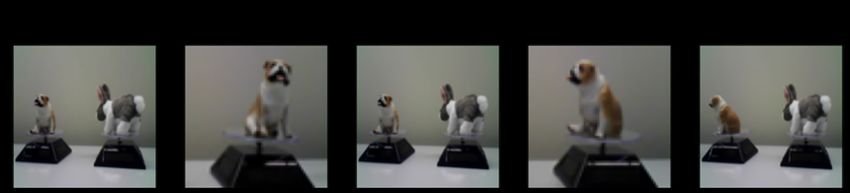
Kingma and Welling [33]) formulation, and decompositions of the VAE objective, for example [19,
31, 8, 7, 35, 6, 14]. GAN-based approaches for disentanglement have been proposed as well [8, 5].

Domain confusion. Our proposed approach is based on the ability to learn an encoding in which
different conditions (i.e., states of the observed factor) are indistinguishable. Such principle has been
in wide use in the machine learning community for domain adaptation tasks [15]. A popular means
to achieve this approximate invariance is via discriminator networks, for example, in [37, 44, 50, 45],
where the high-level mechanism is similar to the one proposed in this work, although specifics may
differ.

3     Problem Formulation
Let X ∈ Rd be a random variable. We assume that X is generated via X = f (S, T ), where f is
an unknown invertible function of two arguments, and S ∈ S and T ∈ T are two random variables
in arbitrary domains, satisfying S ⊥       ⊥ T . We refer to S as the unobserved source that we wish to
recover, to T as the observed condition, and to X as the observed input.
    Let {(si , ti )}ni=1 be n realizations of S × T , and for all i = 1, . . . , n, let xi = f (si , ti ). Given only
input-condition pairs, i.e., {(xi , ti )}ni=1 , we state two goals. First, from analysis standpoint, we aim
to recover the realizations s1 , . . . sn of the unobserved source S. Second, from synthesis standpoint,
for any (new) realization t of T , we aim to to generate an instance x = f (si , t) for any i = 1, . . . , n.

4     Autoencoder Model with Discriminator
To achieve the above goals, we propose using an autoencoder (AE) model (E, D), where the encoder
E maps inputs x to codes s0 (analysis), and the decoder D maps code-condition tuples (s0 , t) to
                                               E                   D
                                               → s0 and (s0 , t) 7−→ x̂. Our approach is illustrated in
input reconstructions x̂ (synthesis), i.e., x 7−
Figure 1.

4.1     Recovery of the Latent Component
Let S 0 = E(X, T ) be a random variable representing the encoder output, and let X̂ = D(S 0 , T ) be
a random variable representing the decoder output.
    Lemma 4.1 establishes that when the autoencoder is trained to perfect reconstruction and the
learned code is independent of the condition, the learned code contains the same information as S,
thus proving that the latent component of interest can be recovered, up to an entropy-preserving
transformation.
Lemma 4.1. Suppose we train the autoencoder model to zero generalization loss, i.e., X̂ = X, and
impose on the code that S 0 ⊥
                            ⊥ T . Then I(S; S 0 ) = H(S) = H(S 0 ).

Proof. Since f is invertible, and S ⊥
                                    ⊥ T , H(X) = H(S) + H(T ). Consider the Markov chain X →
(S 0 , T ) → X̂. By Data Processing Inequality (DPI) I(X; (S 0 , T )) ≥ I(X; X̂) = I(X; X) = H(X),
therefore
                                   I(X; (S 0 , T )) = H(S) + H(T ).                            (1)

                                                         3
Figure 1: The proposed approach. The discriminator is trained to leverage mutual information in
the code s0 and the condition t, via nonlinear correlation or related objectives. The autoencoder is
trained to minimize reconstruction error, while keeping the code and condition independent, thus to
compute code which is equivalent to the latent source s, up to entropy-preserving transformation.

Therefore

                            H(S) + H(T ) = I(X; (S 0 , T ))
                                           = H(X) − H(X|S 0 , T )
                                           = H(S) + H(T ) − H(X|S 0 , T )
                                           = H(S) + H(T ) − H(S|S 0 ),

and thus H(S|S 0 ) = 0, hence I(S; S 0 ) = H(S). It remains to show that H(S) = H(S 0 ). Note that
H(S 0 ) ≥ I(S; S 0 ) = H(S). Finally, considering the encoder, observe that

                                         H(S 0 , T ) ≤ H(X),

which gives H(S 0 ) ≤ H(S) and hence H(S 0 ) = H(S).
    This result has two important consequences. First, it shows that unlike the standard nonlinear
ICA problem, the problem we consider here allows for recovery of the latent independent component
of interest. Second, the result prescribes a recipe for a practical solution, which is presented next.

4.2    System Design
Lemma 4.1 proves that when the autoencoder yields perfect reconstruction and condition-independent
code, the learned code is a recovery of the random variable S, up to entropy-preserving transfor-
mation. Requiring the autoencoder to generate accurate reconstruction of X̂ of X ensures that no
information on S is lost in the encoding process. The independence requirement ensures that the
encoding S 0 does not carry any information in X which is not in S (i.e., is in T ).

                                                  4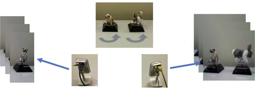
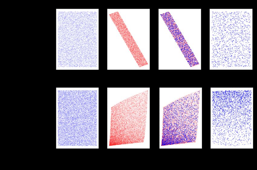
Figure 2: Analysis demonstration. The reconstruction plots show train data in red and reconstructed
test data in blue. The learned code S 0 is a recovery of the latent factor S, up to entropy-preserving
transformation (e.g., an arbitrary monotonic transformation). The approximate independence of
the S 0 and the condition T can be recognized by noticing that the joint density of the code and the
condition is an outer product of the marginal distributions.

   To obtain a code S 0 which is independent of the condition T , we utilize a discriminator network,
aiming to leverage information on T in S 0 for prediction, and train the encoder E to fail the dis-
criminator, in a standard adversarial training fashion. Doing so pushes the learned codes S 0 towards
being a condition-free encoding of X.

4.3    Training Objectives
Broadly, we propose to optimize the following objectives for the discriminator and autoencoder:

                       Ldisc = min Indh (E(x), t)                                                 (2)
                                 h
                        LAE = min [Recon(x, D(E(x))), t) − λIndh (E(x), t)] ,                     (3)
                               E,D

utilizing two objective terms: a reconstruction term (Recon) and an independence term (Ind), where
h denotes the map between the code s0 and the condition t computed by the discriminator, and λ
is a constant balancing between the two terms. Below we specify several optional choices for each
of the terms. The specific choice of reconstruction and independence objective terms in each of the
experiments in this manuscript will be presented in the following section.

Reconstruction. In our experiments, we use standard reconstruction loss functions. In our ex-
periments with images, `1 , MSE and SSIM loss [58] (and combinations of these) are used. `1 loss is

                                                    5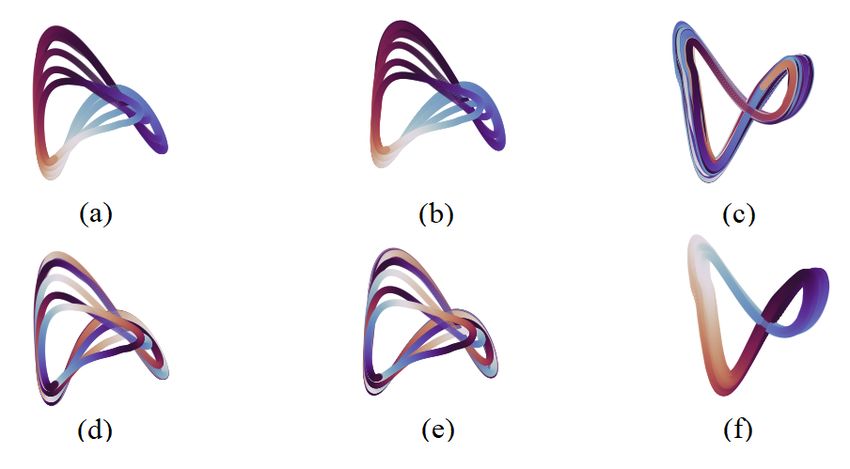
used in our audio experiments, and MSE loss in our experiments with ECG signals.

Independence. In this work we present experimental results in which the discriminator computes
a map t̂ = h(s0 ) and is trained to minimize independence term Indh (s0 , t) (thus to leverage mutual
information in S 0 and T ) as follows.
    When the condition takes values from a finite symbolic set, we train the discriminator as a
classifier, predicting the condition class from the code. This is also known as Domain Confusion
term:
                                   Indh (s0 , t) = Cross Entropy(t̂, t),                          (4)
where s0 = E(x) is the code obtained from the encoder, and t̂ = h(s0 ) is the condition predicted
by the discriminator. Thus, the autoencoder is trained to produce codes that maximize the cross
entropy with respect to the true condition.
   When the condition takes numerical values, we train the classifier as a regression model.
                                       Indh (s0 , t) = −Correl2 (t̂, t),                                 (5)
where the prediction t̂ = h(s0 ) is in R. We remark that this term also equals the R2 term of a simple
regression model, regressing t on t̂. Using this term, the autoencoder is trained to produce codes
for which the squared correlation with the condition is minimized. As t̂ is a nonlinear function of
                                                                         2
s0 , computed via a flexible model such as a neural net, Correl(t̂, t) = 0 implies that S 0 and T are
approximately statistically independent.
     In addition, we also successfully train the discriminator in a contrastive fashion, i.e., to distinguish
between “true tuples”, i.e., tuples (s0 , t) corresponding to samples (s, t) from the joint distribution
PS×T , where x = f (s, t) and s0 = E(x), and “fake tuples”, i.e., tuples (s0 , t), where s0 = E(x) but
x = (s, t̃) with t 6= t̃. The contrastive objective is then:
                                    Indh (s0 , t) = Cross Entropy(ˆl, l),                                (6)
where l is the ground truth true/fake label and ˆl = h(s0i , ti ) is the prediction made by the discrimi-
nator.
   We remark that other possible implementations of the independence criterion can be utilized as
well, e.g., a nonlinear CCA [1, 43] and the Hilbert-Schmidt Independence Criterion (HSIC) [18].

Optimizers: Our proposed approach utilizes two optimizers, one for the autoencoder and one for
the discriminator. The AE optimizer optimizes LAE , by tuning the encoder and decoder weights.
The discriminator optimizer optimizes Ldisc , by tuning the discriminator weights (which determine
the function h). Common practice in training GANs is to call the two optimizers with different
frequencies. We specify the specific choices used in our experiments in Appendix C.

GAN real/ fake discriminator: Optionally, a GAN-like real / fake discriminator can be added
as an additional discriminator in order to encourage generating more realistic inputs. While we have
a successful empirical experience with such GAN discriminators (e.g., in Appendix B), this is not a
core requirement of our proposed approach.

5     Experimental Results
In this section, we demonstrate the efficacy of the proposed approach in various settings, by reporting
experimental results obtained on different data modalities and condition types, in both analysis and
synthesis tasks. We present four applications here and additional two in the appendix.

                                                      6
Figure 3: The rotating figures experiment setup. Bulldog and Bunny rotate in different speeds. The
right camera captures both Bulldog and Bunny, while the left camera captures only Bulldog. Images
from the right camera are considered as the input x, which is generated from two independent factors
– the rotation angles of the figures. Bulldog is considered as the condition t. The goal is to recover
the rotation angle of Bunny, and to manipulate a given input image x by plugging in a different
condition than the one present in the image. The fact that t and x are captured from two different
viewpoints prevents modification of the image simply by pasting Bulldog into x.
Figure 4: The rotating figures experiment. From left to right: (i) the input image to the encoder x,
(ii) the condition t corresponding to Bulldog in x as captured from the viewpoint of the left camera,
(iii) the reconstruction x̂ of x, (iv) a new condition plugged into the decoder, and (v) the resulting
manipulated image.
We begin with a two dimensional analysis demonstration, in which the condition is real-valued.
Second, we demonstrate the usage of our approach for image manipulation, where the condition is
given as an image. Third, the proposed approach is used for voice cloning, which is primarily a
synthesis task with symbolic condition. Fourth, we apply our approach to an ECG analysis task,
using a real-valued heartbeat signal as the condition. Additional experimental results in image
synthesis are described Appendix A and B.
The network architectures and training hyperparameters used in each of the experiments are
described Appendix C. In addition, codes reproducing some of the results in this manuscript are
available at https://github.com/ica-demos.
5.1 2D Analysis Demonstration
In this example we first generate the latent representation of the data by sampling from two indepen-
dent uniform random variables. We then generate the observed data via linear mixing. We consider
one of the latent components as the condition and train the autoencoder to reconstruct the observed
data, while obtaining code which is independent of the condition using the regression objective (5).
7We use `1 as a reconstruction term. The top row in Figure 2 shows the latent, observed and recon-
structed data, as well as the distribution of the condition and the learned code. The bottom row
in Figure 2 shows the results of a similar setup, except for the mixing which is now nonlinear. As
can be seen, the joint distribution of the learned code and the condition is approximately a tensor
product of the marginal distributions, which implies that the latent component is indeed recovered.
5.2 Rotating Figures
In this experiment we use the setup shown in Figure 3, in which two figures, Bulldog and Bunny,
rotate on discs. The rotation speeds are different and are not an integer multiple one of the other.
The figures are recorded by two static cameras, where the right camera captures both Bunny and
Bulldog, while the left camera captures only Bulldog. The cameras operate simultaneously, so that
in each pair of images Bulldog’s position with respect to the table is the same. This dataset was
curated in [38].
We consider images from the right camera (which contain both figures) as the observed input x,
and the images from the left camera (which only show Bulldog) as the condition t. Note that the
input can be considered as generated from two independent sources, namely the rotation angles of
Bulldog and Bunny. The goal is to use x and t to recover the rotation angle s of Bunny1 .
Once training is done, we use the autoencoder to generate new images by manipulating Bulldog’s
rotation angle while preserving Bunny’s. This is done by feeding a (synchronous) (x, t) tuple to the
encoder, obtaining an encoding s0 , sampling an arbitrary condition t̃ and feeding (s0 , t̃) through the
decoder.
We use `1 loss for reconstruction, and contrastive loss (6) to train the discriminator. Namely,
we train the discriminator to distinguish between (image, condition) tuples, which were shot at the
same time, and tuples which were not.
Figure 4 shows an exemplifying result. As can be seen, the learned model disentangles the
rotation angles of Bunny and Bulldog and generates images in which Bunny’s rotation angle is
preserved while Bulldog’s is manipulated.
5.3 Voice Cloning
To demonstrate the application of the proposed method to voice conversion, we run experiments on
a non-parallel corpus, CSTR VCTK Corpus [57], which consists of 109 English speakers with several
accents (e.g., English, American, Scottish, Irish, Indian, etc.). In our experiments, we use a subset
of the corpus containing all the utterances for the first 30 speakers (p225- p256, without p235 and
p242).
We construct the autoencoder to operate on mel spectrograms, using the speaker id as the
condition. The AE architecture was based on Jasper [40] blocks (specific details can be found
in Appendix C). The decoder use a learnable lookup table with 64-dimensional embedding for
each speaker. For the discriminator, we use the same architecture as in [44]. We use `1 loss for
reconstruction, and the discriminator is trained using domain confusion loss (4). Along with the
reconstruction loss, in this experiment we also train a real/fake discriminator, applied to the output
of the decoder. To convert the decoder output to waveform, we use a pre-trained melgan [36] vocoder.
Once the autoencoder is trained, we apply it to convert speech from any speaker to any other
speaker. Some samples of the converted speech are given at https://ica-audio.github.io/. To
evaluate the similarity of the converted voice and the target voice, we use MCD (Mel Cepstral
1 A related work on this dataset was done in [51], although there the goal was the opposite one, i.e., to recover the
common information of the two views, which is the rotation angle of Bulldog.
8Table 1: Voice cloning results: Mel Cepstral Distortion (MCD) in terms of mean (std). PPG, PPG2
results are taken from [47], VQ AVE and PPG GMM results are taken from [12].
Method MCD
TTS Skins [47] 8.76 (1.72)
GLE [12] 7.56
VQ VAE 8.43
PPG GMM 8.57
PPG 9.19 (1.50)
PPG2 9.18 (1.52)
Ours 6.27 (1.44)
Distortion) on a subset of the data containing parallel sentences of multiple speakers. Specifically,
MCD computes the `1 difference between dynamically time warped instance of the converted source
voice and a parallel instance of the target voice, and is a common evaluation metric in voice cloning
research. We remark that the parallel data are used only for evaluation and not to train the model.
We use the script provided at [39] to compute the MCD and compare our proposed approach
to [12, 47] and references therein, which are all considered to be strong baselines, trained on the
VCTK dataset as well. The results, shown in Table 1, demonstrate that our proposed approach
outperforms these strong baselines.
5.4 Fetal ECG extraction
In this experiment we demonstrate the applicability of the proposed approach to non-invasive fetal
electrocardiogram (fECG) extraction, which facilitates the important task of monitoring the fetal
cardiac activity during pregnancy and labor. Following commonly-used non-invasive methods, we
consider extraction of the fECG based on two signals: (i) multi-channel abdominal ECG record-
ings, which consist of a mixture of the desired fECG and the masking maternal electrocardiogram
(mECG), and (ii) thorax ECG recordings, which are assumed to contain only the mECG.
In analogy to our problem formulation (see Section 3), the desired unobserved source s denotes
the fECG, the observed condition t denotes the (thorax) mECG, and the input x denotes the
abdominal ECG.
Dataset. We consider the dataset from [54], which is publicly available2 on PhysioNet [16]. This
dataset was recently published and is part of an ongoing effort to establish a benchmark for non-
invasive fECG extraction methods. The dataset consists of ECG recordings from 60 subjects. Each
recording consists of na = 24 abdominal ECG channels and nt = 3 thorax ECG channels. In
addition, it contains a pulse-wave doppler recording of the fetal heart that serves as a ground-truth.
See Appendix C.6 for more details.
Model training. The input-condition pairs (xi , ti ) are time-segments of the abdominal ECG
recordings (xi ∈ Rna ×nT ) and the thorax ECG recordings (ti ∈ Rnt ×nT ), where the length of the
time-segments is set to nT = 2, 000 (4 seconds). We train a separate model for each subject based
on a collection of n input-condition pairs {(xi , ti )}ni=1 of time-segments.
The encoder is based on a convolutional neural network (CNN), so that the obtained codes
s0i = E(xi , ti ) ∈ Rnd ×nT are time-segments, where the dimension of the code is set to nd = 5. For
more details on the architecture, model training, and hyperparameters selection, see Appendix C.6.
We note that the training is performed in an unsupervised manner, i.e., we use the ground-truth
doppler signal only for evaluation and not during training.
2 https://physionet.org/content/ninfea/1.0.0/
9Table 2: fECG extraction results. In the leftmost column, we present Rx , and in the other columns
we present Rs0 achieved by the different methods.
# of Subject Input Ours ADALINE ESN LMS RLS
Top 5 2.23 (3.23) 6.86 (1.98) 6.46 (2.54) 1.99 (1.08) 2.60 (1.60) 1.03 (0.70)
Top 10 1.20 (2.41) 5.43 (2.02) 4.22 (2.94) 1.19 (1.10) 1.56 (1.53) 0.75 (0.56)
Top 20 0.66 (1.75) 3.53 (2.44) 2.59 (2.63) 0.71 (0.91) 0.89 (1.26) 0.51 (0.46)
All 0.30 (1.17) 1.84 (2.16) 1.32 (2.08) 0.36 (0.68) 0.40 (0.94) 0.26 (0.38)
Figure 5: Example of an input-condition pair (xi , ti ) and the obtained code s0i . The duration of the
presented time segment is 2 sec. (a) The abdominal channels xi (for brevity only 5 channels are
presented). (b) The thorax channels ti . (c) The obtained code s0i . The time intervals associated
with the fetal and maternal QRS complexes are marked by red and green frames, respectively.
Qualitative evaluation. In Figure 5 we present an example of an input-condition pair (xi , ti )
and the obtained code s0i = E(xi , ti ). We see that the abdominal channels consist of a mixture of
the fECG and the mECG, where the fECG is significantly less dominant than the mECG and might
even be completely absent from some of the channels. In addition, we see that the thorax channels
are affected by the mECG only. Lastly, we see that the obtained code captures the fECG without
any noticeable trace of the mECG.
In Figure 6, we present the projections of 1, 000 sequentially-sampled inputs xi (abdominal
channels), conditions ti (thorax channels), and their codes s0i = E(xi , ti ) on their respective 3
principal components. We color the projected points by the periodicity of the mECG (top row),
computed from the thorax channels, and by the periodicity of the fECG (bottom row), computed
from the ground-truth doppler signals. We see that the PCA of the abdominal and thorax channels
are similar, implying that the mECG dominates the mixture. In addition, we see that the color of
the PCA of the abdominal and thorax channels according to the mECG ((a) and (b)) is similar and
smooth, unlike the color by the fECG ((d) and (e)). In contrast, the PCA of the code is different
((c) and (f)) and only the color by the fECG is smooth (f), indicating that the code captures the
fECG without a significant trace of the mECG, as desired.
Baselines. We consider four baselines taken from a recent review [28]. Specifically, we focus on
methods that utilize reference thorax channels. The first two baselines are based on adaptive filtering,
which is considered to be the traditional approach for fECG extraction: least mean squares (LMS)
and recursive least squares (RLS). This approach was first introduced by Widrow et al. [59], and it
is still considered to be relevant in recent studies [42, 60, 55]. The third baseline is adaptive linear
network (ADALINE). ADALINE utilizes neural networks adaptable to the nonlinear time-varying
properties of the ECG signal [29]. The fourth baseline is based on echo state network (ESN) [26].
10Figure 6: PCA of the samples colored by the mECG (top row) and fECG (bottom row). (a) and
(d) the PCA of the inputs xi . (b) and (e) the PCA of the conditions ti . (c) and (f) and PCA of the
obtained codes s0i .
Quantitative evaluation. To the best of our knowledge, there is no gold-standard nor definitive
evaluation metrics for fECG extraction. Here, based on the ground-truth doppler signal, we quantify
the enhancement of the fECG and the suppression of the mECG as follows.
First, we compute the principal component of the input xi . Second, we compute the one-sided
auto-correlation of the principal component, and denote it by Axi . Then, we quantify the average
(f ) Pns (f ) (f )
presence of the fECG in the inputs xi by computing: Āx = n1s i=1 Axi (τi ), where τi denotes
the periods of the fECG obtained from the doppler signals, and ns denotes the number of time
(m) Pns (m) (m)
segments in the evaluated recording. Similarly, we compute Āx = n1s i=1 Axi (τi ), where τi
denotes the periods of the mECG obtained from the thorax signals. Finally, to quantify the relative
Ā(f )
presences of the signals, we compute the ratio Rx = (m) x
. We apply the same procedure to the
Āx
codes s0i , resulting in Rs0 . When evaluating the baselines, we consider the signals obtained after the
mECG cancellation as the counterparts of our code signals.
In Table 2, we present the average ratios in the input, code, and baselines over all the subjects
(see Appendix C.6 for results per subject). We note that not all the subjects in the dataset include
a noticeable fECG in the abdominal recordings. Therefore, we present results over subsets of top
k subjects showing highest average ratios Rx . We see that our method significantly enhances the
fECG with respect to the mixture, and it outperforms the tested baselines.
6 Conclusion
In this paper, we present an autoencoder-based approach for single independent component recovery.
The considered problem consists of observed data (mixture) generated from two independent com-
ponents: one observed and the other hidden that needs to be recovered. We theoretically show that
this ICA-related recovery problem can be accurately solved, in the sense that the hidden component
is recovered up to an entropy-preserving function, by an autoencoder equipped with a discrimina-
tor. In addition, we demonstrate the relevance of the problem and the performance of the proposed
solution on several tasks, involving image manipulation, voice cloning, and fetal ECG extraction.
11References
[1] Andrew, G., Arora, R., Bilmes, J., and Livescu, K. (2013). Deep canonical correlation analysis.
In International conference on machine learning, pages 1247–1255. PMLR.
[2] Belkin, M. and Niyogi, P. (2003). Laplacian eigenmaps for dimensionality reduction and data
representation. Neural computation, 15(6):1373–1396.
[3] Blau, Y. and Michaeli, T. (2018). The perception-distortion tradeoff. In Proceedings of the IEEE
Conference on Computer Vision and Pattern Recognition, pages 6228–6237.
[4] Blei, D. M., Ng, A. Y., and Jordan, M. I. (2003). Latent dirichlet allocation. the Journal of
machine Learning research, 3:993–1022.
[5] Brakel, P. and Bengio, Y. (2017). Learning independent features with adversarial nets for non-
linear ica. arXiv preprint arXiv:1710.05050.
[6] Burgess, C. P., Higgins, I., Pal, A., Matthey, L., Watters, N., Desjardins, G., and Lerchner, A.
(2018). Understanding disentangling in beta-vae. arXiv preprint arXiv:1804.03599.
[7] Chen, R. T., Li, X., Grosse, R., and Duvenaud, D. (2018). Isolating sources of disentanglement
in variational autoencoders. arXiv preprint arXiv:1802.04942.
[8] Chen, X., Duan, Y., Houthooft, R., Schulman, J., Sutskever, I., and Abbeel, P. (2016). Infogan:
Interpretable representation learning by information maximizing generative adversarial nets. arXiv
preprint arXiv:1606.03657.
[9] Clevert, D.-A., Unterthiner, T., and Hochreiter, S. (2015). Fast and accurate deep network
learning by exponential linear units (elus). arXiv preprint arXiv:1511.07289.
[10] Coifman, R. R. and Lafon, S. (2006). Diffusion maps. Applied and computational harmonic
analysis, 21(1):5–30.
[11] Comon, P. (1994). Independent component analysis, a new concept? Signal processing,
36(3):287–314.
[12] Ding, S. and Gutierrez-Osuna, R. (2019). Group latent embedding for vector quantized varia-
tional autoencoder in non-parallel voice conversion. In INTERSPEECH, pages 724–728.
[13] Eriksson, J. and Koivunen, V. (2004). Identifiability, separability, and uniqueness of linear ica
models. IEEE signal processing letters, 11(7):601–604.
[14] Esmaeili, B., Wu, H., Jain, S., Bozkurt, A., Siddharth, N., Paige, B., Brooks, D. H., Dy, J.,
and Meent, J.-W. (2019). Structured disentangled representations. In The 22nd International
Conference on Artificial Intelligence and Statistics, pages 2525–2534. PMLR.
[15] Ganin, Y., Ustinova, E., Ajakan, H., Germain, P., Larochelle, H., Laviolette, F., Marchand,
M., and Lempitsky, V. (2016). Domain-adversarial training of neural networks. The journal of
machine learning research, 17(1):2096–2030.
[16] Goldberger, A. L., Amaral, L. A., Glass, L., Hausdorff, J. M., Ivanov, P. C., Mark, R. G.,
Mietus, J. E., Moody, G. B., Peng, C.-K., and Stanley, H. E. (2000). Physiobank, physiotoolkit,
and physionet: components of a new research resource for complex physiologic signals. circulation,
101(23):e215–e220.
12[17] Gresele, L., Rubenstein, P. K., Mehrjou, A., Locatello, F., and Schölkopf, B. (2020). The in-
complete rosetta stone problem: Identifiability results for multi-view nonlinear ica. In Uncertainty
in Artificial Intelligence, pages 217–227. PMLR.
[18] Gretton, A., Bousquet, O., Smola, A., and Schölkopf, B. (2005). Measuring statistical depen-
dence with hilbert-schmidt norms. In International conference on algorithmic learning theory,
pages 63–77. Springer.
[19] Higgins, I., Matthey, L., Pal, A., Burgess, C., Glorot, X., Botvinick, M., Mohamed, S., and
Lerchner, A. (2016). beta-vae: Learning basic visual concepts with a constrained variational
framework.
[20] Hotelling, H. (1933). Analysis of a complex of statistical variables into principal components.
Journal of educational psychology, 24(6):417.
[21] Hyvarinen, A. and Morioka, H. (2016). Unsupervised feature extraction by time-contrastive
learning and nonlinear ica. arXiv preprint arXiv:1605.06336.
[22] Hyvarinen, A. and Morioka, H. (2017). Nonlinear ica of temporally dependent stationary
sources. In Artificial Intelligence and Statistics, pages 460–469. PMLR.
[23] Hyvärinen, A. and Oja, E. (2000). Independent component analysis: algorithms and applica-
tions. Neural networks, 13(4-5):411–430.
[24] Hyvärinen, A. and Pajunen, P. (1999). Nonlinear independent component analysis: Existence
and uniqueness results. Neural networks, 12(3):429–439.
[25] Hyvarinen, A., Sasaki, H., and Turner, R. (2019). Nonlinear ica using auxiliary variables and
generalized contrastive learning. In The 22nd International Conference on Artificial Intelligence
and Statistics, pages 859–868. PMLR.
[26] Jaeger, H. (2001). The “echo state” approach to analysing and training recurrent neural
networks-with an erratum note. Bonn, Germany: German National Research Center for In-
formation Technology GMD Technical Report, 148(34):13.
[27] Jordan, M. I. (1998). Learning in graphical models, volume 89. Springer Science & Business
Media.
[28] Kahankova, R., Martinek, R., Jaros, R., Behbehani, K., Matonia, A., Jezewski, M., and Behar,
J. A. (2019). A review of signal processing techniques for non-invasive fetal electrocardiography.
IEEE reviews in biomedical engineering, 13:51–73.
[29] Kahankova, R., Martinek, R., Mikolášová, M., and Jaroš, R. (2018). Adaptive linear neuron
for fetal electrocardiogram extraction. In 2018 IEEE 20th International Conference on e-Health
Networking, Applications and Services (Healthcom), pages 1–5. IEEE.
[30] Khemakhem, I., Kingma, D., Monti, R., and Hyvarinen, A. (2020). Variational autoencoders
and nonlinear ica: A unifying framework. In International Conference on Artificial Intelligence
and Statistics, pages 2207–2217. PMLR.
[31] Kim, H. and Mnih, A. (2018). Disentangling by factorising. In International Conference on
Machine Learning, pages 2649–2658. PMLR.
13[32] Kingma, D. P. and Ba, J. (2014). Adam: A method for stochastic optimization. arXiv preprint
arXiv:1412.6980.
[33] Kingma, D. P. and Welling, M. (2013). Auto-encoding variational bayes. arXiv preprint
arXiv:1312.6114.
[34] Koller, D. and Friedman, N. (2009). Probabilistic graphical models: principles and techniques.
MIT press.
[35] Kumar, A., Sattigeri, P., and Balakrishnan, A. (2017). Variational inference of disentangled
latent concepts from unlabeled observations. arXiv preprint arXiv:1711.00848.
[36] Kumar, K., Kumar, R., de Boissiere, T., Gestin, L., Teoh, W. Z., Sotelo, J., de Brébisson, A.,
Bengio, Y., and Courville, A. (2019). Melgan: Generative adversarial networks for conditional
waveform synthesis. arXiv preprint arXiv:1910.06711.
[37] Lample, G., Zeghidour, N., Usunier, N., Bordes, A., Denoyer, L., and Ranzato, M. (2017).
Fader networks: Manipulating images by sliding attributes. arXiv preprint arXiv:1706.00409.
[38] Lederman, R. R. and Talmon, R. (2018). Learning the geometry of common latent variables
using alternating-diffusion. Applied and Computational Harmonic Analysis, 44(3):509–536.
[39] Li, C., Shi, J., Zhang, W., Subramanian, A. S., Chang, X., Kamo, N., Hira, M., Hayashi, T.,
Boeddeker, C., Chen, Z., and Watanabe, S. (2021). ESPnet-SE: End-to-end speech enhancement
and separation toolkit designed for ASR integration. In Proceedings of IEEE Spoken Language
Technology Workshop (SLT), pages 785–792. IEEE.
[40] Li, J., Lavrukhin, V., Ginsburg, B., Leary, R., Kuchaiev, O., Cohen, J. M., Nguyen, H., and
Gadde, R. T. (2019). Jasper: An end-to-end convolutional neural acoustic model. arXiv preprint
arXiv:1904.03288.
[41] Locatello, F., Bauer, S., Lucic, M., Raetsch, G., Gelly, S., Schölkopf, B., and Bachem, O. (2019).
Challenging common assumptions in the unsupervised learning of disentangled representations.
In international conference on machine learning, pages 4114–4124. PMLR.
[42] Martinek, R., Kahankova, R., Nazeran, H., Konecny, J., Jezewski, J., Janku, P., Bilik, P., Zidek,
J., Nedoma, J., and Fajkus, M. (2017). Non-invasive fetal monitoring: A maternal surface ecg
electrode placement-based novel approach for optimization of adaptive filter control parameters
using the lms and rls algorithms. Sensors, 17(5):1154.
[43] Michaeli, T., Wang, W., and Livescu, K. (2016). Nonparametric canonical correlation analysis.
In International conference on machine learning, pages 1967–1976. PMLR.
[44] Mor, N., Wolf, L., Polyak, A., and Taigman, Y. (2018). A universal music translation network.
arXiv preprint arXiv:1805.07848.
[45] Nachmani, E. and Wolf, L. (2019). Unsupervised singing voice conversion. arXiv preprint
arXiv:1904.06590.
[46] Pearson, K. (1901). Liii. on lines and planes of closest fit to systems of points in space. The
London, Edinburgh, and Dublin philosophical magazine and journal of science, 2(11):559–572.
[47] Polyak, A., Wolf, L., and Taigman, Y. (2019). Tts skins: Speaker conversion via asr. arXiv
preprint arXiv:1904.08983.
14[48] Roweis, S. T. and Saul, L. K. (2000). Nonlinear dimensionality reduction by locally linear
embedding. science, 290(5500):2323–2326.
[49] Schölkopf, B., Smola, A., and Müller, K.-R. (1998). Nonlinear component analysis as a kernel
eigenvalue problem. Neural computation, 10(5):1299–1319.
[50] Shaham, U. (2018). Batch effect removal via batch-free encoding. bioRxiv, page 380816.
[51] Shaham, U. and Lederman, R. R. (2018). Learning by coincidence: Siamese networks and
common variable learning. Pattern Recognition, 74:52–63.
[52] Sorrenson, P., Rother, C., and Köthe, U. (2020). Disentanglement by nonlinear ica with general
incompressible-flow networks (gin). arXiv preprint arXiv:2001.04872.
[53] Sprekeler, H., Zito, T., and Wiskott, L. (2014). An extension of slow feature analysis for
nonlinear blind source separation. The Journal of Machine Learning Research, 15(1):921–947.
[54] Sulas, E., Urru, M., Tumbarello, R., Raffo, L., Sameni, R., and Pani, D. (2021). A non-invasive
multimodal foetal ecg–doppler dataset for antenatal cardiology research. Scientific Data, 8(1):1–
19.
[55] Swarnalath, R. and Prasad, D. (2010). A novel technique for extraction of fecg using multi
stage adaptive filtering. Journal of Applied Sciences, 10(4):319–324.
[56] Tenenbaum, J. B., De Silva, V., and Langford, J. C. (2000). A global geometric framework for
nonlinear dimensionality reduction. science, 290(5500):2319–2323.
[57] Veaux, C., Yamagishi, J., MacDonald, K., et al. (2017). Cstr vctk corpus: English multi-speaker
corpus for cstr voice cloning toolkit. University of Edinburgh. The Centre for Speech Technology
Research (CSTR).
[58] Wang, Z., Bovik, A. C., Sheikh, H. R., and Simoncelli, E. P. (2004). Image quality assessment:
from error visibility to structural similarity. IEEE transactions on image processing, 13(4):600–
612.
[59] Widrow, B., Glover, J. R., McCool, J. M., Kaunitz, J., Williams, C. S., Hearn, R. H., Zei-
dler, J. R., Dong, J. E., and Goodlin, R. C. (1975). Adaptive noise cancelling: Principles and
applications. Proceedings of the IEEE, 63(12):1692–1716.
[60] Wu, S., Shen, Y., Zhou, Z., Lin, L., Zeng, Y., and Gao, X. (2013). Research of fetal ecg
extraction using wavelet analysis and adaptive filtering. Computers in biology and medicine,
43(10):1622–1627.
[61] Yildirim, O., San Tan, R., and Acharya, U. R. (2018). An efficient compression of ecg signals
using deep convolutional autoencoders. Cognitive Systems Research, 52:198–211.
[62] Zhu, J.-Y., Park, T., Isola, P., and Efros, A. A. (2017). Unpaired image-to-image translation
using cycle-consistent adversarial networks. In Proceedings of the IEEE international conference
on computer vision, pages 2223–2232.
15Figure 7: The colored MNIST experiment, using the color (left) and digit label (right) as condition.
In each of the plots, the leftmost column show the input x to the encoder, and the next column
shows the reconstruction. The remaining columns show conversion to each of the condition classes.
A Colored MNIST experiment
In this experiment we used a colored version of the MNIST handwritten image dataset, obtained
by converting the images to RGB format and coloring each digit with an arbitrary color from
{red, green, blue}.
We ran two experiments on this dataset. In the first one we considered the color as the condition.
This setup perfectly meets the model assumptions, as each colored image was generated by choosing
an arbitrary color at random (t) and coloring the original grayscale image (s). In the second
experiment we set the condition to be the digit label. This corresponds to a data generation process
in which handwriting characteristics (e.g., line thickness, orientation) and color are independent of
the digit label. While the color was indeed chosen independently of any other factor, independence
of the handwriting characteristics and the digit label is debateable, as for example, orientation may
depend on the specific digits (e.g., ’1’ is often written in a tilted fashion, while this is not the case
for other digits).
The condition t was incorporated into decoder by modulating the feature maps before each
convolutional layer. The discriminator was trained using domain confusion loss. As a reconstruction
term we used (pixel-wise) binary cross entropy.
Once the autoencoder was trained, we used it to manipulate the images by plugging to the
decoder arbitrary condition and generating new data. Figure 7 shows examples of reconstructions
and manipulation for both experiments. In the left panel (showing the results for condition=color)
we can see that very high quality reconstruction and conversion were achieved, implying that the
learned code did not contain color information, while preserving most of the information of the
grayscale image, as desired. The right panel (showing results for condition=digit label) displays
similar results, although of somewhat worse conversion quality, as this setting does not fully fit the
assumptions taken in this work. Yet, the code clearly captures most dominant characteristics of the
handwriting.
16Figure 8: Image Domain Conversion experiment. Left: Conversion results on the oranges2apples
dataset. Right: Conversion from Cezanne to photo (up) and Van Goch to photo (down).
B Image Domain Conversion
In this experiment we apply the proposed approach to some of the datasets introduced in [62]. Here
the condition is the domain (e.g., orange / apple). We use a combination of `1 and SSIM loss for
reconstruction and domain confusion for independence. In addition to reconstruction loss, we also
use a GAN-like real/fake discriminator to slightly improve perceptual loss [3]. Some results are shown
in Figure 8. While an interested reader might wonder why oranges are converted to red oranges
rather than apples, we remark that as much as the condition specifies the type of fruit (orange /
apple) throughout this dataset it also specifies its color (orange / red), which, by Ockham’s razor,
is a somewhat simpler description of the separation between the two domains. Therefore the image
manipulation made by the model can be interpreted as a domain conversion.
C Technical Details
C.1 2D demonstration
In this experiment we used MLP architectures for all networks, where each of the encoder, decoder
and discriminator consisted of three hidden layers, each of size 64. Identity and softplus activations
were used for the linear and nonlinear mixing experiments, respectively. The discriminator was
regularized using r1 loss, computed every eight steps. The model was trained for 100 epochs on a
dataset of 15,000 points. To balance between the reconstruction and independence terms we used
λ = 0.05. The autoencoder optimizer was called every 5th step. A Jupyter notebook running this
demo is available at https://github.com/ica-demos/.
17C.2 MNIST Experiment
In this experiment each of the encoder and decoder consisted of three colvolutional layers, of 16, 32
and 64 kernels and ReLU activations. The discriminator had a MLP architecture with 128 units in
each layer. The condition was incorporated into the decoder via modulation, utilizing a learnable
lookup table of class embeddings of dimension 64. In this experiment we also used an additionale
discriminator, trained in a GAN fashion to distinguish between real and generated images. During
training this discriminator was also trained on swapped data, i.e., codes that were fed to the decoder
with a random condition. This discriminator has three convolution layers and was trained with
standard non-saturating GAN loss. The system was trained for 50 epochs, with λ = 0.01 and the
real/fake discriminator loss term was added to the LAE in (2) with coefficient of 0.001. A Jupyter
notebook running this demo is available at https://github.com/ica-demos/.
C.3 Rotating Figures
The images x were of size 128 × 128 pixels and the conditions were of size 64×64. In the encoder
images were passed through two downsampling blocks and two residual blocks. ResNet encoding
models were applied to the condition and the images (separately), before the their feature maps
were concatenated and passed through several additional ResNet blocks. In the decoder conditions
were downsampled once and passed through two residual blocks, before being concatenated to the
codes and fed through two more residual blocks. The decoder and discriminator have a similar
architecture. We use `1 as reconstruction loss. The system was trained for 120 epochs on a dataset
containing 10,000 instances, using λ = 1.05, and the autoencoder was trained every 5th step.
C.4 Image Domain Conversion
In this experiment the encoder and decoder’s architectures were inspired by the cycleGAN [62]
ResNet generator architecture, splitting the generator to to encoder and decoder. The decoder was
enlarged with modulation layer before each convolutional layer. The class embeddings were of size
512. As in the MNIST experiment, GAN-like real / fake discriminator was used here as well. The
system was trained for 200 epochs, on the datasets downloaded from the cyclegan official repository3 .
We used λind = λrf = 0.1 for both discriminators. The autoencoder was trained every 5th step. A
Jupyter notebook running this demo is available at https://github.com/ica-demos/.
C.5 Voice Conversion
The encoder receives mel-filterbank features calculated from windows of 1024 samples with a 256
samples overlap, and outputs a latent representation of the source speech. The network is constructed
from downsampling by factor 2 1D convolution layer with ReLU followed by 30 Jasper [40] blocks,
where each sub-block applies a 1D convolution, batch norm, ReLU, and dropout. All sub-blocks
in a block have the same number of output channels which we set to 256. The decoder is also a
convolutional neural network which receives as input the latent representation produced by encoder
and the target speaker id as the condition. The condition was then mapped to a learnable embedding
in R64 concatenated to the encoder output by repeating it along the temporal dimension. The
concatenated condition is passed through 1D convolution layer with stride 1 followed by a leaky-
ReLU activation with a leakiness of 0.2 and 1D transposed convolution with stride 2 for upsampling
to the original time dimension. The discriminator was trained using domain confusion loss (4). We
3 https://github.com/junyanz/pytorch-CycleGAN-and-pix2pix/blob/master/datasets/download_cyclegan_
dataset.sh
18exploit the same structure as in [44]: four 1D-convolution layers, with the ELU [9] nonlinearity.
The system was trained for 2000 epochs, which took 8 days on a simple GTX 1080 GPU. We used
λ = 1, both optimizers were called every training step.
C.6 ECG Analysis
C.6.1 Dataset
The dataset consists of 60 entries from 39 voluntary pregnant womens. Each entry is composed
of recordings from 27 ECG channels and a synchronised recording from a trans-abdominal pulse-
wave doppler (PWD) of the fetal’s heart. The recordings’ lengths vary from 7.5 seconds to 119.8
seconds (with average length of 30.6 seconds ± 20.6 seconds). The ECG recordings were sampled
by the TMSi Porti7 system with a frequency-sampling rate of 2KHz . The PWD recordings were
acquired using the Philips iE33 ultrasound machine. The obtained video was converted into a 1D
time-series using a processing scheme based on envelope detection. The code for this processing
scheme was provided as a Matlab-script by the authors of [54]. For convenience, we uploaded the
obtained 1D time-series after applying the provided Matlab-script, and it is available at https:
//github.com/ica-demos/ECG/tree/master/Data.
C.6.2 Pre-proecssing and model implementation
In the following we provide a detailed description of the pre-processing steps and the implemen-
tation of the model. For convenience, all the parameters and hyperparameters are summarized in
Table 3. The recording of subjects 1-20 were used for hyperparameters selection. These subjects
were discarded in the objective evaluation reported in Table 2.
Pre-processing. The raw ECG recordings were filtered by a median filter with a window length
of nm = 2, 048 (1 second) to remove the baseline drift. In addition, we apply a notch filter to
remove the 50Hz powerline noise and a low-pass filter with a cut-off frequency of Fc = 125Hz.
Finally, we downsample the signal to frequency-sampling rate of Fs = 500Hz. The doppler signal
was pre-processed using the script provided by the dataset’s owners. No further operations were
performed.
Implementation details. The encoder module E(X) is implemented using a convolutional neural
network (CNN): Rna ×nT → Rnd ×nT . This choice of architecture is inspired by the architecture
proposed by [61] for the benefit of ECG compression, and it is described in details in Table 4.
The implementation of the decoder module D(S 0 , T ) is based on a deconvolutional neural network
(dCNN): R(nd +nt )×nT → Rna ×nT . This decoder is applied to the concatenation of the code signal
and the thorax signal, where the concatenation is along the first dimension. The exact architecture
is described in details in Table 5.
The discrimination module Indh (S 0 , T ) is implemented via an additional CNN h(T ) : Rnt ×nT →
Rnd ×nT . h(T ) shares the same architecture as E(X), except the first convolutional layer which has
nt input channels rather than na . Specifically, Indh (S 0 , T ) = Ind(S 0 , h(T )), where Ind(x, y) is a
|x|e |y|e
scale-invariant version of the MSE loss function: Ind(x, y) = ||x|| F
− ||y|| F F
, and | · |e denotes an
element-wise operation of absolute value. We remark that other possibilities can be considered as
well.
Lastly, the reconstruction module is simply implemented via the standard MSE loss: Recon(x, y) =
x − y F.
19Table 3: List of parameters and hyperparameters used in the ECG analysis. Parameters are listed
in the upper part of the table, while hyperparameters are listed in the lower part of the table.
Notation Description Value
na Number of abdominal channels 24
nt Number of thorax channels 3
nm Window length of the median-filter 2, 000
Fc Cut-off frequency 5 · 104
Fs Frequency-sample 500
nd Dimensioanlity of the code 5
n Number condition-pairs for training 5 · 104
b Batch size 32
lr Learning rate 10−4
λ Objective independecy factor 0.01
β Interleaving independecy factor 5
Table 4: Layers consisting the encoder E(X) in the ECG analysis.
Layer No. of filters Activation Output
No
name × kernel size function size
1 1D Conv 8×3 Tanh 2000 × 8
2 1D Conv 8×5 Tanh 2000 × 8
3 Batch Norm. - - 2000 × 8
4 1D Conv 8×3 Tanh 2000 × 8
5 Batch Norm. - - 2000 × 8
6 1D Conv 8 × 11 Tanh 2000 × 8
7 1D Conv 8 × 13 Tanh 2000 × 8
8 1D Conv nd × 3 Tanh 2000 × nd
C.6.3 Training process
We train a model for each subject. The training data is a collection of n input-condition pairs
{(xi , ti )}ni=1 , where each input-condition pair (xi , ti ) is a time-segment that was selected from the
ECG recording at a randomly drawn offset and n is a hyperparameter indicating the number of ran-
domly drawn training examples. We use two optimizers that operate in an interleaved (adverserial-
like) fashion. Specifically, for each update step of the second optimizer we perform β update steps of
the first optimizer, where β = 5 is a hyperparameter. The first optimizer updates h(T ) and aims to
maximize the dependency between the condition and the code. The second optimizer updates E(X)
and D(S 0 , T ) and has two objectives – minimizing the reconstruction loss while preventing the first
optimizer from succeeding to maximize the dependency loss. Hence, encouraging the optimization
process to converge to a “condition-free” code. The proportion between these two objectives is
controlled by the hyperparameter λ = 0.01 that multiplies the second objective term. The losses
obtained by the two optimizers are denoted by Ldisc and LAE in eq. (2).
Both optimizers are implemented using the Adam algorithm [32] with a fixed learning rate of
lr = 10−4 , β = (0.9, 0.999) and a bach-size of b = 32.
20Table 5: Layers consisting the decoder D(S 0 , T ) in the ECG analysis. “T.Conv” denotes a transposed
convolution layer.
Layer No. of filters Activation Output
No
name × kernel size function size
1 1D T.Conv 8×3 Tanh 2000 × 8
2 1D T.Conv 8 × 13 Tanh 2000 × 8
3 1D T.Conv 8×3 Tanh 2000 × 8
4 1D T.Conv 8×5 Tanh 2000 × 8
5 1D T.Conv na × 3 Tanh 2000 × na
C.6.4 Qualitative evaluation
Here, we describe in detail the procedure presented in Section 5.4 in the paper. First, we produce a
code s0i for each input-condition pair (xi , ti ). Then, we column-stack each matrix in the set {s0i }1,000
i=1
and project the obtained set of vectors to a 3D space using principal component analysis (PCA). We
repeat the same procedure for {xi }1,000
i=1 . We color the projected points in two manners: according
to the fECG signal and according to the mECG signal. The color of the ith sample representing the
fECG (mECG) signal is computed as follows: {mod(i, τ (f ) )}1,000i=1 ({mod(i, τ
(m) 1,000
)}i=1 ), where τ (f )
(m)
(τ ) denotes the period of the fECG (mECG) obtained from the doppler signal (thorax recordings).
C.6.5 Objective evaluation
The results presented in Section 5.4 are averaged over subsets of subjects. In Table 6 we present the
results for each subject.
21Table 6: fECG extraction results for each subject.
Subject Input Ours ADALINE ESN LMS RLS
1 0.11 (0.10) 0.74 (1.63) 0.51 (0.51) 0.05 (0.16) 0.00 (0.00) 0.20 (0.16)
2 0.13 (0.12) 0.51 (1.90) 0.17 (0.58) 0.07 (0.12) 0.00 (0.00) -0.02 (0.10)
3 0.10 (0.13) 0.49 (0.90) 0.56 (0.59) 0.45 (0.33) 0.47 (0.33) 0.04 (0.14)
4 0.15 (0.22) 0.69 (0.68) 0.10 (0.70) 0.15 (0.50) 0.07 (0.15) 0.08 (0.22)
5 7.89 (0.12) 0.74 (1.04) -0.01 (0.69) 0.22 (0.36) 0.07 (0.72) 0.04 (0.13)
6 0.11 (0.09) 0.58 (1.14) 0.39 (0.54) 0.14 (0.22) 0.34 (0.45) 0.10 (0.15)
7 0.10 (0.11) 0.07 (0.99) 1.04 (0.84) 0.32 (0.28) 0.60 (0.41) 0.09 (0.10)
8 -0.00 (0.26) 0.94 (0.69) 0.26 (0.48) 0.18 (0.79) 0.00 (0.00) 0.17 (0.28)
10 0.10 (0.10) 4.41 (1.48) 1.46 (2.01) 0.22 (0.25) 0.01 (0.02) 0.03 (0.12)
11 0.09 (0.12) 0.56 (1.73) 0.68 (0.63) 0.11 (0.17) 0.00 (0.00) 0.15 (0.22)
13 -0.05 (0.08) 1.35 (0.50) 1.08 (1.23) 0.03 (0.50) 0.00 (0.01) 0.58 (0.30)
14 -0.03 (0.05) 3.60 (3.18) 8.82 (4.39) 1.85 (1.59) 3.17 (2.50) 0.90 (0.54)
15 0.13 (0.39) 0.52 (0.90) 0.36 (0.67) 0.29 (1.04) 0.14 (0.82) 0.28 (0.22)
16 0.04 (0.20) 0.80 (1.57) 0.20 (0.61) 0.09 (0.51) 0.00 (0.00) -0.03 (0.13)
17 0.03 (0.23) 1.31 (0.45) 0.29 (0.50) -0.06 (0.32) 0.00 (0.00) 0.58 (0.54)
18 0.03 (0.05) 0.50 (0.82) 0.58 (1.34) 0.04 (0.14) -0.01 (0.02) 0.12 (0.19)
19 0.11 (0.08) 0.86 (0.94) 1.03 (0.99) 0.19 (0.23) 0.00 (0.00) 0.22 (0.14)
20 0.17 (0.15) 0.86 (0.94) 0.24 (0.52) 0.14 (0.38) 0.45 (0.54) 0.28 (0.39)
21 0.23 (0.15) 0.40 (0.45) 0.28 (0.45) 0.24 (0.34) 0.36 (0.45) 0.44 (0.24)
22 1.17 (0.59) 1.41 (1.10) 1.00 (1.65) 1.14 (0.69) 3.56 (2.09) 2.28 (2.57)
23 0.16 (0.24) 0.82 (1.31) 0.17 (1.11) 0.23 (1.40) 0.01 (0.03) 0.03 (0.08)
24 0.05 (0.11) 0.92 (1.05) 0.19 (0.74) 0.48 (0.65) 0.53 (0.35) 0.28 (0.25)
25 -0.05 (0.08) 0.36 (0.38) 0.81 (0.60) 0.30 (0.36) 0.40 (0.53) -0.05 (0.20)
26 0.09 (0.66) 0.67 (1.08) 0.56 (0.69) 0.23 (0.40) 0.17 (0.34) 0.11 (0.14)
27 0.02 (0.12) 0.46 (0.71) 0.34 (0.43) 0.10 (0.32) 0.20 (0.40) 0.09 (0.19)
28 -0.01 (0.09) 1.88 (1.80) 1.55 (1.49) 0.02 (0.18) 0.00 (0.00) 0.15 (0.12)
29 -0.07 (0.04) 0.83 (0.90) 1.09 (0.97) -0.10 (0.06) 0.24 (0.04) 0.04 (0.18)
30 0.09 (0.11) 8.14 (3.21) 0.95 (0.99) 0.43 (0.55) 0.83 (0.97) 0.34 (0.30)
31 0.10 (0.13) 1.06 (0.60) 0.33 (0.33) 0.05 (0.24) 0.01 (0.00) 0.01 (0.20)
32 0.03 (0.22) 1.27 (1.04) 0.25 (0.24) -0.06 (0.22) 0.00 (0.00) -0.05 (0.23)
33 0.03 (0.20) 0.30 (0.35) 0.35 (0.24) 0.02 (0.14) 0.00 (0.00) -0.09 (0.13)
37 0.09 (0.18) 0.82 (0.70) 0.02 (0.72) 0.21 (0.40) 0.00 (0.00) 0.15 (0.11)
39 0.13 (0.17) 9.57 (3.24) 9.16 (1.67) 0.12 (0.17) 0.05 (0.02) 0.48 (0.24)
41 0.08 (0.08) 5.66 (7.76) 4.28 (3.49) 0.13 (0.34) 0.00 (0.00) 0.32 (0.51)
43 -0.07 (0.04) 1.21 (0.80) 1.61 (1.00) 0.29 (0.38) 0.56 (0.37) 0.35 (0.26)
44 -0.06 (0.08) 1.42 (1.03) 1.09 (1.36) 0.00 (0.80) 0.09 (0.09) 0.27 (0.19)
45 1.69 (0.43) 4.30 (4.73) 0.56 (1.57) 0.95 (1.81) 1.02 (0.68) 0.77 (0.77)
46 0.18 (0.11) 3.47 (2.77) 6.45 (5.37) 3.62 (1.68) 4.45 (4.05) 0.17 (0.15)
48 0.06 (0.21) 3.40 (1.68) 3.12 (2.79) 2.37 (1.44) 0.03 (0.02) 0.24 (0.55)
50 0.13 (0.27) 0.50 (0.79) 0.52 (0.65) 0.21 (0.32) 0.00 (0.00) 0.01 (0.08)
51 0.13 (0.24) 0.24 (0.48) 3.59 (2.63) 0.13 (0.27) 0.00 (0.00) 0.65 (0.26)
55 0.15 (0.16) 4.65 (5.32) 2.15 (1.78) 0.10 (0.18) 0.01 (0.00) 0.04 (0.15)
56 0.14 (0.13) 4.24 (1.60) 0.77 (0.66) 0.04 (0.23) 0.04 (0.11) 0.08 (0.15)
58 0.09 (0.31) 6.29 (4.99) -0.01 (0.67) 0.15 (0.53) 0.17 (0.62) 0.45 (0.33)
59 0.09 (0.09) 0.79 (0.88) 0.34 (0.71) 0.14 (0.23) 0.00 (0.00) 0.35 (0.17)
22You can also read