Self-Replication via Tile Self-Assembly (Extended Abstract)
←
→
Page content transcription
If your browser does not render page correctly, please read the page content below
Self-Replication via Tile Self-Assembly
(Extended Abstract)
Andrew Alseth         #
University of Arkansas, Fayetteville, AR, USA

Daniel Hader        #
University of Arkansas, Fayetteville, AR, USA

Matthew J. Patitz #
University of Arkansas, Fayetteville, AR, USA

      Abstract
In this paper we present a model containing modifications to the Signal-passing Tile Assembly Model
(STAM), a tile-based self-assembly model whose tiles are capable of activating and deactivating glues
based on the binding of other glues. These modifications consist of an extension to 3D, the ability
of tiles to form “flexible” bonds that allow bound tiles to rotate relative to each other, and allowing
tiles of multiple shapes within the same system. We call this new model the STAM*, and we present
a series of constructions within it that are capable of self-replicating behavior. Namely, the input
seed assemblies to our STAM* systems can encode either “genomes” specifying the instructions for
building a target shape, or can be copies of the target shape with instructions built in. A universal
tile set exists for any target shape (at scale factor 2), and from a genome assembly creates infinite
copies of the genome as well as the target shape. An input target structure, on the other hand, can
be “deconstructed” by the universal tile set to form a genome encoding it, which will then replicate
and also initiate the growth of copies of assemblies of the target shape. Since the lengths of the
genomes for these constructions are proportional to the number of points in the target shape, we also
present a replicator which utilizes hierarchical self-assembly to greatly reduce the size of the genomes
required. The main goals of this work are to examine minimal requirements of self-assembling
systems capable of self-replicating behavior, with the aim of better understanding self-replication in
nature as well as understanding the complexity of mimicking it.
2012 ACM Subject Classification Theory of computation → Models of computation; General and
reference → General conference proceedings
Keywords and phrases Algorithmic self-assembly, tile assembly model, self-replication
Digital Object Identifier 10.4230/LIPIcs.DNA.27.3
Related Version Full Version: https://arxiv.org/abs/2105.02914 [2]

Funding Andrew Alseth: This author’s work was supported in part by NSF grant CAREER-1553166.
Daniel Hader: This author’s work was supported in part by NSF grant CAREER-1553166.
Matthew J. Patitz: This author’s work was supported in part by NSF grant CAREER-1553166.

 1      Introduction

1.1     Background and motivation
Research in tile based self-assembly is typically focused on modeling the computational and
shape-building capabilities of biological nano-materials whose dynamics are rich enough to
allow for interesting algorithmic behavior. Polymers such as DNA, RNA, and poly-peptide
chains are of particular interest because of the complex ways in which they can fold and
bind with both themselves and others. Even when only taking advantage of a small subset
of the dynamics of these materials, with properties like binding and folding generally being
restricted to very manageable cases, tile assembly models have been extremely successful in
exhibiting vast arrays of interesting behavior [45, 48, 17, 11, 13, 38, 50, 16, 5, 8, 15]. Among
            © Andrew Alseth, Daniel Hader, and Matthew J. Patitz;
            licensed under Creative Commons License CC-BY 4.0
27th International Conference on DNA Computing and Molecular Programming (DNA 27).
Editors: Matthew R. Lakin and Petr Šulc; Article No. 3; pp. 3:1–3:22
                   Leibniz International Proceedings in Informatics
                   Schloss Dagstuhl – Leibniz-Zentrum für Informatik, Dagstuhl Publishing, Germany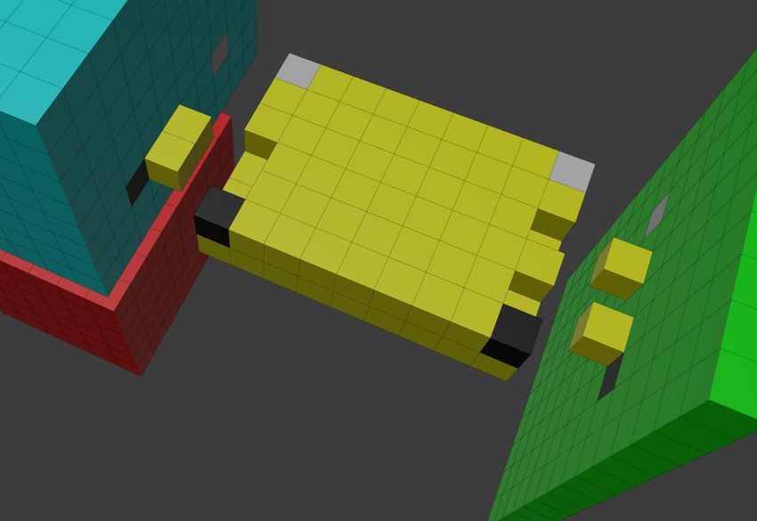
3:2   Self-Replication

      other things, a typical question in the realm of algorithmic tile assembly asks what the
      minimal set of requirements is to achieve some desired property. Such questions can range
      from very concrete, such as “how many distinct tile types are necessary to construct specific
      shapes?”, to more abstract such as “under what conditions is the construction of self-similar
      fractal-like structures possible?”. Since the molecules inspiring many tile assembly models
      are used in nature largely for the purpose of self-replication of living organisms, a natural tile
      assembly question is thus whether or not such behavior is possible to model algorithmically.
          In this paper we show that we can define a model of tile assembly in which the complexities
      of self-replication type behavior can be captured, and provide constructions in which such
      behavior occurs. We define our model with the intention of it (1) being hopefully physically
      implementable in the (near) future, and (2) using as few assumptions and constraints as
      possible. Our constructions therefore provide insight into understanding the basic rules under
      which the complex dynamics of life, particularly self-replication, may occur.
          We chose to use the Signal-passing Tile Assembly Model (STAM) as a basis for our
      model, which we call the STAM*, because (1) there has been success in physically realizing
      such systems [41] and potential exists for further, more complex, implementations using well-
      established technologies like DNA origami [44, 39, 52, 3, 4] and DNA strand displacement [43,
      51, 47, 54, 53, 7], and (2) the STAM allows for behavior such as cooperative tile attachment as
      well as detachment of subassemblies. We modify the STAM by bringing it into 3 dimensions
      and making a few simplifying assumptions, such as allowing multiple tile shapes and tile
      rotation around flexible glues and removing the restriction that tiles have to remain on a fixed
      grid. Allowing flexibility of structures and multiple tile shapes provides powerful new dynamics
      that can mimic several aspects of biological systems and suffice to allow our constructions
      to model self-replicating behavior. Prior work, theoretical [36] and experimental [46], has
      focused on the replication of patterns of bits/letters on 2D surfaces, as well as the replication
      of 2D shapes in a model using staged assembly [1], or in the STAM [27]. However, all of these
      are fundamentally 2D results and our 3D results, while strictly theoretical, are a superset
      with constructions capable of replicating all finite 2D and 3D patterns and shapes.
          Biological self-replication requires three main categories of components: (1) instructions,
      (2) building blocks, and (3) molecular machinery to read the instructions and combine
      building blocks in the manner specified by the instructions. We can see the embodiment
      of these components as follows: (1) DNA/RNA sequences, (2) amino acids, and (3) RNA
      polymerase, transfer RNA, and ribosomes, among other things. With our intention to study
      the simplest systems capable of replication, we started by developing what we envisioned
      to be the simplest model that would provide the necessary dynamics, the STAM*, and
      then designed modular systems within the STAM* which each demonstrated one or more
      important behaviors related to replication. Quite interestingly, and unintentionally, our
      constructions resulted in components with strong similarities to biological counterparts. As
      our base encoding of the instructions for a target shape, we make use of a linear assembly
      which has some functional similarity to DNA. Similar to DNA, this structure also is capable
      of being replicated to form additional copies of the “genome”. In our main construction, it is
      necessary for this linear sequence of instructions to be “transcribed” into a new assembly
      which also encodes the instructions but which is also functionally able to facilitate translation
      of those instructions into the target shape. Since this sequence is also degraded during the
      growth of the target structure, it shares some similarity with RNA and its role in replication.
      Our constructions don’t have an analog to the molecular machinery of the ribosome, and
      can therefore “bootstrap” with only singleton copies of tiles from our universal set of tiles in
      solution. However, to balance the fact that we don’t need preexisting machinery, our building
      blocks are more complicated than amino acids, instead being tiles capable of a constant
      number of signal operations each (turning glues on or off due to the binding of other glues).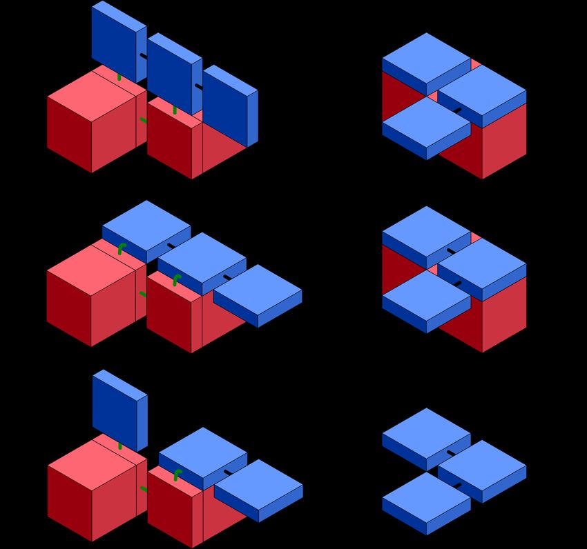
A. Alseth, D. Hader, and M. J. Patitz                                                                   3:3

1.2     Our results
Beyond the definition of the STAM* as a new model, we present a series of STAM* construc-
tions. They are designed and presented in a modular fashion, and we discuss the ways in
which they can be combined to create various (self-)replicating systems.

1.2.1    Genome-based replicator
We first develop an STAM* tileset which functions as a simple self-replicator (in Section 3)
that begins from a seed assembly encoding information about a target structure, a.k.a. a
genome, and grows arbitrarily many copies of the genome and target structure, a.k.a. the
phenotype. This tileset is universal for all 3D shapes comprised of 1 × 1 × 1 cubes when they
are inflated to scale factor 2 (i.e. each 1 × 1 × 1 block in the shape is represented by a cube
of 2 × 2 × 2 tiles). This construction requires a genome whose length is proportional to the
number of cube tiles in the phenotype; for non-trivial shapes the genome is a constant factor
longer in order to follow a Hamiltonian path through an arbitrary 3D shape at scale factor 2.
This is compared to the Soloveichik and Winfree universal (2D) constructor [49] where a
“genome” is optimally shortened, but the scale factor of blocks is much larger.
    The process by which this occurs contains analogs to natural systems. We progress
from a genome sequence (acting like DNA), which is translated into a messenger sequence
(somewhat analogous to RNA), that is modified and consumed in the production of tertiary
structures (analogous to proteins). We have a number of helper structures that fuel both the
replication of the genome and the translation of the messenger sequence.

1.2.2    Deconstructive self-replicator
In Section 4, we construct an STAM* tileset that can be used in systems in which an
arbitrarily shaped seed structure, or phenotype, is disassembled while simultaneously forming
a genome that describes its structure. This genome can then be converted into a linear
genome (of the form used for the first construction) to be replicated arbitrarily and can
be used to construct a copy of the phenotype. We show that this can be done for any
3D shape at scale factor 2 which is sufficient, and in some cases necessary, to allow for a
Hamiltonian path to pass through each point in the shape. This Hamiltonian path, among
other information necessary for the disassembly and, later, reassembly processes, is encoded
in the glues and signals of the tiles making up the phenotype. We then show how, using
simple signal tile dynamics, the phenotype can be disassembled tile by tile to create a
genome encoding that same information. Additionally, a reverse process exists so that once
the genome has been constructed from a phenotype, a very similar process can be used to
reconstruct the phenotype while disassembling the genome.
     In sticking with the DNA, RNA, protein analogy, this disassembly process doesn’t have a
particular biological analog; however, this result is important because it shows that we can
make our system robust to starting conditions. That is, we can begin the self-replication
process at any stage be it from the linear genome, “kinky genome” (the messenger sequence
from the first construction), or phenotype. Finally, since this construction requires the
phenotype to encode information in its glues and signals, we show that this can be computed
efficiently using a polynomial time algorithm given the target shape. This not only shows that
the STAM* systems can be described efficiently for any target shape via a single universal
tile set, but that results from intractable computations aren’t built into our phenotype (i.e.
we’re not “cheating” by doing complex pre-computations that couldn’t be done efficiently
by a typical computationally universal system). Due to space constraints we only include a
result about the necessity for deconstruction in a universal replicator in the online version [2].

                                                                                                     DNA 27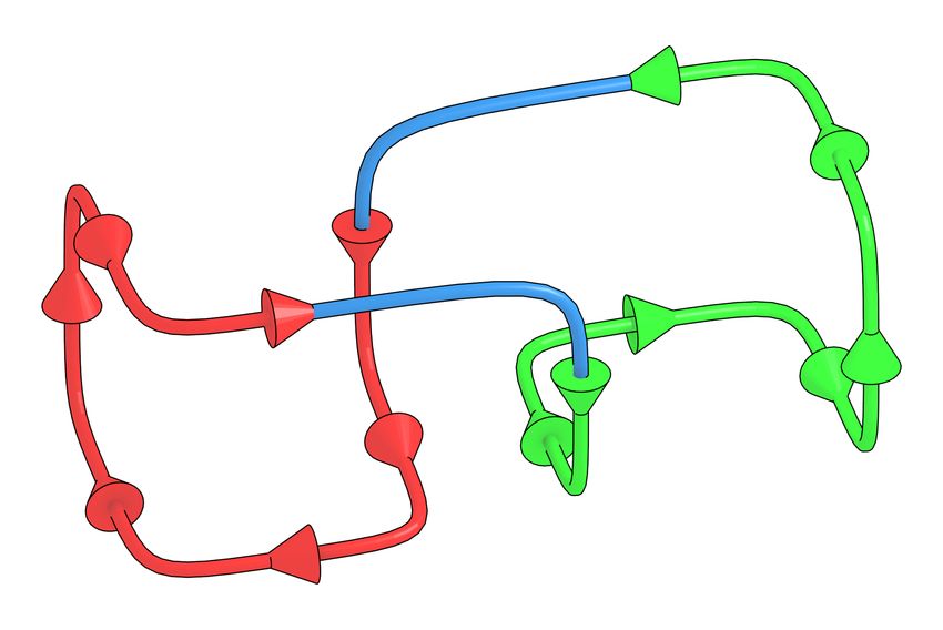
3:4   Self-Replication

      1.2.3    Hierarchical assembly-based replicator
      For our final construction, in Section 5, our aims were twofold. First, we wanted to compress
      the genome so that its total length is much shorter than the number of tiles in the target
      shape. Second, we wanted to more closely mimic the biological process in which individual
      proteins are constructed via the molecular machinery, and then they are released to engage
      in a hierarchical self-assembly process in which proteins combine to form larger structures.
          Biological genomes are many orders of magnitude smaller than the organisms which they
      encode, but for our previous constructions the genomes are essentially equivalent in size to the
      target structures. Our final construction is presented in a “simple” form in which the general
                                                                      1
      scaling approximately results in a genome which is length n 3 for a target structure of size
      n. However, we discuss relatively simple modifications which could, for some target shapes,
      result in genome sizes of approximately log n, and finally we discuss a more complicated
      extension (which also consumes a large amount of “fuel”, as opposed to the base constructions
      which consume almost no fuel) that can achieve asymptotically optimal encoding.

      1.2.4    Combinations and permutations of constructions
      Due to length restrictions for this version of the paper, and our desire to present what we
      found to be the “simplest” systems capable of combining to perform self-replication, there are
      several additions to our results which we only briefly mention. For instance, to make our first
      construction (in Section 3) into a standalone self-replicator, and one which functions slightly
      more like biological systems, the input to the system, i.e. the seed assembly, could instead be
      a copy of the target structure with a genome “tail” attached to it. The system could function
      very similarly to the construction of Section 3 but instead of genome replication and structure
      building being separated, the genome could be replicated and then initiate the growth of a
      connected messenger structure so that once the target structure is completed, the genome is
      attached. Thus, the input assembly would be completely replicated, and be a self-replicator
      more closely mirroring biology where the DNA along with the structure cause the DNA to
      replicate itself and the structure. Attaching the genome to the structure is a technicality that
      could satisfy the need to have a single seed assembly type, but clearly it doesn’t meaningfully
      change the behavior. At the end of Section 5 we discuss how that construction could be
      combined with those from Sections 3 and 4, as well as further optimized. This version of
      the paper contains high-level overviews of the definition of the STAM* as well as of the
      results. Full technical details for each section can be found in the full version online [2] in
      the corresponding sections of the technical appendix.

       2      Preliminaries

      In this section we define the notation and models used throughout the paper.
          We define a 3D shape S ⊂ Z 3 as a finite connected set of 1 × 1 × 1 cubes (a.k.a. unit
      cubes) which define an arbitrary polycube, i.e. a shape composed of unit cubes connected
      face to face where each cube represents a voxel (3-D pixel) of S. For each shape S, we
      assume a canonical translation and rotation of S so that, without loss of generality, we can
      reference the coordinates of each of its voxels and directions of its surfaces, or faces. We
      say a unit cube is scaled by factor c if it is replaced by a c × c × c cube composed of c3 unit
      cubes. Given an arbitrary 3D shape S, we say S is scaled by factor c if every unit cube of S
      is scaled by factor c and those scaled cubes are arranged in the shape of S. We denote a
      shape S scaled by factor c as S c .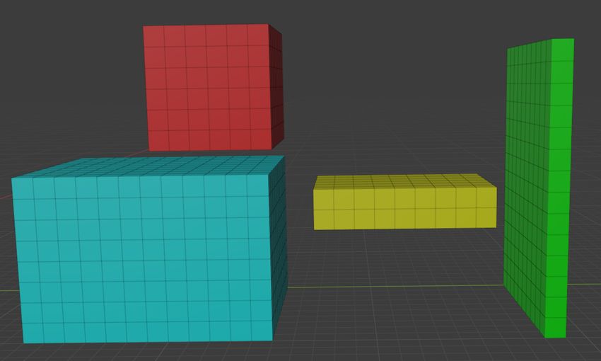
A. Alseth, D. Hader, and M. J. Patitz                                                                     3:5

2.1    Definition of the STAM*
The 3D Signal-passing Tile Assembly Model* (3D-STAM*, or simply STAM*) is a general-
ization of the STAM [40, 20, 26, 37] (that is similar to the model in [30, 31]) in which (1)
the natural extension from 2D to 3D is made (i.e. tiles become 3-dimensional shapes rather
than 2-dimensional squares), (2) multiple tile shapes are allowed, (3) tiles are allowed to flip
and rotate [11, 28], and (4) glues are allowed to be rigid (as in the aTAM, 2HAM, STAM,
etc., meaning that when two adjacent tiles bind to each other via a rigid glue, their relative
orientations are fixed by that glue) or flexible (as in [18]) so that even after being bound tiles
and subassemblies are free rotate with respect to tiles and subassemblies to which they are
bound by bending or twisting around a “joint” in the glue. (This would be analogous to rigid
glues forming as DNA strands combine to form helices with no single-stranded gaps, while
flexible glues would have one or more unpaired nucleotides leaving a portion of single-stranded
DNA joining the two tiles, which would be flexible and rotatable.) See Figure 1a for a simple
example. These extensions make the STAM* a hybrid model of those in previous studies of
hierarchical assembly [8, 12, 14, 42, 29], 3D tile-based self-assembly [10, 22, 6, 24], systems
allowing various non-square/non-cubic tile types [19, 23, 11, 21, 25, 35], and systems in which
tiles can fold and rearrange [18, 34, 32, 33].
    Due to space constraints, we now provide a high-level overview of several aspects of the
STAM* model, and full definitions can be found in the online version [2].
    The basic components of the model are tiles. Tiles bind to each other via glues. Each
glue has a glue type that specifies its domain (which is the string label of the glue), integer
strength, flexibility (a boolean value with true meaning flexible and false meaning rigid),
and length (representing the length of the physical glue component). A glue is an instance of
a glue type and may be in one of three states at any given time, {latent,on,off}. A pair
of adjacent glues are able to bind to each other if they have complementary domains and are
both in the on state, and do so with strength equal to their shared strength values (which
must be the same for all glues with the same label l or the complementary label l∗ ).
    A tile type is defined by its 3D shape (and although arbitrary rotation and translation in
  3
R are allowed, each is assigned a canonical orientation for reference), its set of glues, and its
set of signals. Its set of glues specify the types. locations, and initial states of its glues. Each
signal in its set of signals is a triple (g1 , g2 , δ) where g1 and g2 specify the source and target
glues (from the set of the tile type’s glues) and δ ∈ {activate,deactivate}. Such a signal
denotes that when glue g1 forms a bond, an action is initiated to turn glue g2 either on (if
δ == activate) or off (otherwise). A tile is an instance of a tile type represented by its
type, location, rotation, set of glue states (i.e. latent,on or off for each), and set of signal
states. Each signal can be in one of the signal states {pre,firing,post}. A signal which
has never been activated (by its source glue forming a bond) is in the pre state. A signal
which has activated but whose action has not yet completed is in the firing state, and if
that action has completed it is in the post state. Each signal can “fire” only one time, and
each glue which is the target of one or more signals is only allowed to make the following
state transitions: (1) latent → on, (2) on → off, or (3) latent → off.
    We use the terms assembly and supertile, interchangeably, to refer to the full set of
rotations and translations of either a single tile (the base case) or a collection of tiles which
are bound together by glues. A supertile is defined by the tiles it contains (which includes
their glue and signal states) and the glue bonds between them. A supertile may be flexible
(due to the existence of a cut consisting entirely of flexible glues that are co-linear and there
being an unobstructed path for one subassembly to rotate relative to the other), and we call
each valid positioning of it sets of subassemblies a configuration of the supertile. A supertile
may also be translated and rotated while in any valid configuration. We call a supertile in a
particular configuration, rotation, and translation a positioned supertile.

                                                                                                       DNA 27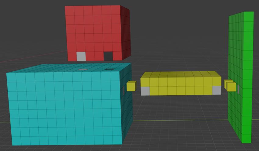
3:6   Self-Replication

          Each supertile induces a binding graph, a multigraph whose vertices are tiles, with an
      edge between two tiles for each glue which is bound between them. The supertile is τ -stable
      if every cut of its binding graph has strength at least τ , where the weight of an edge is the
      strength of the glue it represents. That is, the supertile is τ -stable if cutting bonds of at
      least summed strength of τ is required to separate the supertile into two parts.
          For a supertile α, we use the notation |α| to represent the number of tiles contained in
      α. The domain of a positioned supertile α, written dom α, is the union of the points in R3
      contained within the tiles composing α. Let α be a positioned supertile. Then, for ⃗v ∈ R3 , we
      define the partial function α(⃗v ) = t where t is the tile containing ⃗v if ⃗v ∈ dom α, otherwise it
      is undefined. Given two positioned supertiles, α and β, we say that they are equivalent, and
      we write α ≈ β, if for all ⃗v ∈ R3 α(⃗v ) and β(⃗v ) both either return tiles of the same type, or
      are undefined. We say they’re equal, and write α ≡ β, if for all ⃗v ∈ R3 α(⃗v ) and β(⃗v ) either
      both return tiles of the same type having the same glue and signal states, or are undefined.

                     (a)                                       (b)

          Figure 1 (a) Example showing flat and cubic tiles, and possible behavior of a flexible glue allowing
      the blue tile to fold upward, away from the red cubic tile, or down against it. (b) The glue lengths
      in our constructions: (1) length 2ϵ rigid bonds between cubic tiles, (2) length 0 rigid bonds between
                                                                                                       √
      flat and cubic tiles (as though one tile’s glue strand binds into a cavity), and (3) length 3 2 ϵ/2
      flexible glues between flat tiles.

          An STAM* tile assembly system, or TAS, is defined as T = (T, C, τ ) where T is a finite
      set of tile types, C is an initial configuration, and τ ∈ N is the minimum binding threshold
      (a.k.a. temperature) specifying the minimum binding strength that must exist over the sum
      of binding glues between two supertiles in order for them to attach to each other. The initial
      configuration C = {(S, n) | S is a supertile over the tiles in T and n ∈ N ∪ ∞ is the number
      of copies of S}. Note that for each s ∈ S, each tile α = (t, ⃗l, S, γ) ∈ s has a set of glue states
      S and signal states γ. By default, it is assumed that every tile in every supertile of an initial
      configuration begins with all glues in the initial states for its tile type, and with all signal
      states as pre, unless otherwise specified. The initial configuration C of a system T is often
      simply given as a set of supertiles, which are also called seed supertiles, and it is assumed
      that there are infinite counts of each seed supertile as well as of all singleton tile types in T .
      If there is only one seed supertile σ, we will we often just use σ rather than C.

      2.1.1     Overview of STAM* dynamics
      An STAM* system T = (T, C, τ ) evolves nondeterministically in a series of (a possibly
      infinite number of) steps. Each step consists of randomly executing one of the following
      actions: (1) selecting two existing supertiles which have configurations allowing them to
      combine via a set of neighboring glues in the on state whose strengths sum to strength ≥ τ
      and combining them via a random subset of those glues whose strengths sum to ≥ τ (and
      changing any signals with those glues as sources to the state firing if they are in state pre),
A. Alseth, D. Hader, and M. J. Patitz 3:7
or (2) randomly select two adjacent unbound glues of a supertile which are able to bind, bind
them and change attached signals in state pre to firing, or (3) randomly select a supertile
which has a cut < τ (due to glue deactivations) and cause it to break into 2 supertiles along
that cut, or (4) randomly select a signal on some tile of some supertile where that signal is in
the firing state and change that signal’s state to post, and as long as its action (activate
or deactivate) is currently valid for the signal’s target glue, change the target glue’s state
appropriately.1 Although at each step the next choice is random, it must be the case that no
possible selection is ever ignored infinitely often.
Given an STAM* TAS T = (T, C, τ ), a supertile is producible, written as α ∈ A[T ], if
either it is a single tile from T , or it is the result of a (possibly infinite) series of combinations
of pairs of finite producible assemblies (which have each been positioned so that they do not
overlap and can be τ -stably bonded), and/or breaks of producible assemblies. A supertile
α is terminal, written as α ∈ A□ [T ], if (1) for every β ∈ A[T ], α and β cannot be τ -stably
attached, (2) there is no configuration of α in which a pair of unbound complementary glues
in the on state are able to bind, and (3) no signals of any tile in α are in the firing state.
In this paper, we define a shape as a connected subset of Z3 to both simplify the definition
of a shape and to capture the notion that to build an arbitrary shape out of a set of tiles
we will actually approximate it by “pixelating” it. Therefore, given a shape S, we say that
assembly α has shape S if α has only one valid configuration (i.e. it is rigid) and there exist
(1) a rotation of α and (2) a scaling of S, S ′ , such that the rotated α and S ′ can be translated
to overlap where there is a one-to-one and onto correspondence between the tiles of α and
cubes of S ′ (i.e. there is exactly 1 tile of α in each cube of S ′ , and none outside of S ′ ).2
▶ Definition 1. We say a shape X self-assembles in T with waste size c, for c ∈ N, if there
exists terminal assembly α ∈ A□ [T ] such that α has shape X, and for every α ∈ A□ [T ],
either α has shape X, or |α| ≤ c. If c == 1, we simply say X self-assembles in T .
▶ Definition 2. We call an STAM* system R = (T, C, τ ) a shape self-replicator for shape S
if C consists exactly of infinite copies of each tile from T as well as of a single supertile σ of
shape S, there exists c ∈ N such that S self-assembles in R with waste size c, and the count
of assemblies of shape S increases infinitely.
▶ Definition 3. We call an STAM* system R = (T, C, τ ) a self-replicator for σ with waste
size c if C consists exactly of infinite copies of each tile from T as well as of a single supertile
σ, there exists c ∈ N such that for every terminal assembly α ∈ A□ [T ] either (1) α ≈ σ, or
(2) |α| ≤ c, and the count of assemblies ≈ σ increases infinitely.3 If c == 1, we simply say
R is a self-replicator for σ.
The multiple aspects of STAM* tiles and systems give rise to a variety of metrics with
which to characterize and measure the complexity of STAM* systems, beyond metrics seen
for models such as the aTAM or even STAM. For a brief discussion, please see the online
version [2].
1
The asynchronous nature of signal firing and execution is intended to model a signalling process which
can be arbitrarily slow or fast. Please see the online version [2] for more details.
2
In this paper we only consider completely rigid assemblies for target shapes, since the target shapes are
static. We could also target “reconfigurable shapes, i.e. sets of shapes, but don’t do so in this paper.
Also, it could be reasonable to allow multiple tiles in each pixel location as long as the correct overall
shape is maintained, but we don’t require that.
3
We use ≈ rather than ≡ since otherwise either both the seed assemblies and produced assemblies are
terminal, meaning nothing can attach to a seed assembly and the system can’t evolve, or neither are
terminal and it becomes difficult to define the product of a system. However, our construction in
Section 4 can be modified to produce assemblies satisfying either the ≈ or ≡ relation with the seed
assemblies.
DNA 273:8 Self-Replication
2.1.2 STAM* conventions used in this paper
Although the STAM* is a highly generalized model allowing for variety in tile shapes,
glue lengths, etc., throughout this paper all constructions are restricted to the following
conventions.
1. All tile types have one of two shapes (shown in Figure 1a):
a. A cubic tile is a tile whose shape is a 1 × 1 × 1 cube.
b. A flat tile is a tile whose shape is a 1 × 1 × ϵ rectangular prism, where ϵ < 1 is a small
constant.
c. We call a 1 × 1 face of a tile a full face, and a 1 × ϵ face is called a thin face.
2. Glue lengths are the following (and are shown in Figure 1b):
a. All rigid glues between cubic tiles, as well as between thin faces of flat tiles, are length
2ϵ.
b. All rigid glues between cubic and flat tiles are length 0. (Note that this could be
implemented via the glue strand of one tile extending into the tile body of the other
tile in order to bind, thus allowing the tile surfaces to be adjacent without spacing
between the faces.)
√
c. All flexible glues are length 23 2ϵ. 4
Given that rigidly bound cubic tiles cannot rotate relative to each other, for convenience
we often refer to rigidly bound tiles as though they were on a fixed lattice. This is easily
done by first choosing a rigidly bound cubic tile as our origin, then using the location ⃗l,
orientation matrix R, and rigid glue length g, put in one-to-one correspondence with each
vector ⃗v in Z3 , the vector ⃗l + gR⃗v . Once we define an absolute coordinate system in this way,
we refer to the directions in 3-dimensional space as North (+y), East (+x), South (−y), West
(−x), Up (+z), and Down (−z), abbreviating them as N, E, S, W, U, and D, respectively.
3 A Genome Based Replicator
We now present our first construction in the STAM*, in which a “universal” set of tiles will
cause a pre-formed seed assembly encoding a Hamiltonian path through a target structure,
which we call the genome, to replicate infinitely many copies of itself as well as build infinitely
many copies of the target structure at temperature 2. We consider 4 unique structures
which are generated/utilized as part of the self-replication process: σ, µ, µ′ , and π. The seed
assembly, σ, is composed of a connected set of flat tiles considered to be the genome. Let π
represent an assembly of the target shape encoded by σ. µ is an intermediate “messenger”
structure directly copied from σ, which is modified into µ′ to assemble π. We split T into
subsets of tiles, T = {Tσ ∪ Tµ ∪ Tφ ∪ Tπ }. Tσ are the tiles used to replicate the genome, Tµ
are the tiles used to create the messenger structure, Tπ are the cubic tiles which comprise
the phenotype π, and Tφ are the set of tiles which combine to make fuel structures used in
both the genome replication process and conversion of µ to µ′ . We denote this universal
self-assembling system as R = {T, σ, 2}
The tile types which make up this replicator are carefully designed to prevent spurious
structures and enforce two key properties for the self-replication process. First, a genome
is never consumed during replication, allowing for exponential growth in the number of
4
These glue lengths were chosen so that (1) rigidly bound cubic tiles could each have a flat tile bound to
each of their sides if needed and (2) so that two flat tiles attached to diagonally adjacent rigid tiles
could be attached via a flexible glue.A. Alseth, D. Hader, and M. J. Patitz 3:9
completed genome copies. Second, the replication process from messenger to phenotype
strictly follows µ → µ′ → π; each step in the assembly process occurs only after the prior
structure is in its completed form. This prevents unexpected geometric hindrances which
could block progression of any further step. Complete details of T are located in [2].
3.1 Replication of the genome
The minimal requirements to generate copies of σ in R are the following: (1) for all individual
tile types s ∈ σ, s ∈ Tσ , (2) the last tile is the end tile E, and (3) the first tile in σ is a start
tile in the set (S + , S − ). However, for the shape-self replication of S one additional property
must hold: (4) σ encodes a Hamiltonian path which ends on an exterior cubic tile. We define
the genome to be “read” from left to right; given requirements (2) and (3), the leftmost tile
in a genome is a start tile and the rightmost is an end tile. (4) can be guaranteed by scaling
S up to S 2 and utilizing the algorithm in Section 4.3, selecting a cubic tile on the exterior as
a start for the Hamiltonian path and then reversing the result. This requirement ensures the
possibility of cubic tile diffusion into necessary locations at all stages of assembly.
(a) (b)
Figure 2 (a) In step 0 (before replication begins) both fuel and tiles from Tσ bind to σ. Step 1
indicates the fuel tile binding with the leftmost S + tile in σ ′ , propagating the binding of tiles
from west to east indicated by blue arrow on the ++ tile. Step 2 begins after all σ ′ glues are
bound by strength-1, leading to the propagation of a second glue binding σ ′ from east to west.
Additionally, glues on the north face of σ ′ tiles are activated and glues on the south face binding to
σ are deactivated once they have a strength-2 connection to. Step 3 demonstrates the detachment –
once the second glue binds to the fuel duple (φ1 , φ2 ) signals propagate to detach from σ and σ ′ . (b)
Process of translation: the information encoded in σ is copied to µ by a mapping of tiles via glue
domains. Green glues on µ and µ′ are flexible. One kink-ase (red) is used to convert µ to µ′ .
Figure 9a (located in A.1) is a template for the tile set required for the replication of an
arbitrary genome. The process of replicating a genome σ into a new copy σ ′ demonstrated in
Figure 2a is carried out left to right, initiated by a fuel assembly which is jettisoned after all
tiles in σ ′ are connected with strength 2. This allows for the genome σ to be copied without
itself being used up or firing signals, leading to exponential growth. Full detail is available in
the online version [2].
3.2 Translation of σ to µ
Translation is defined as the process by which the Hamiltonian path encoded in σ is built
into a new messenger assembly µ. Since the signals to attach and detach µ from σ are fully
contained in the tiles of Tµ , translation continues as long as Tµ tiles remain in the system.
We note that the translation process can occur at the same time as σ is replicating. This
causes no unwanted geometric hindrances as demonstrated in Figure 9b.
DNA 273:10 Self-Replication
3.2.1 Placement of µ tiles
Messenger tiles from the set Tµ attach to σ as soon as complementary glues on the back flat
face of σ are activated after the binding of the fuel duple φ to σ ′ . The process of building
µ does not require a fuel structure to continue, as the messenger tiles have built-in signals
to deactivate the glues on µ which attach µ to σ. This allows for a genome to replicate the
messenger structure without itself being consumed in any manner. Once a flat tile in µ is
bound to its eastern neighbor, signals are fired from the eastern glues to deactivate the glue
connecting µ to σ. This leaves µ as its own separate assembly when every tile has attached
to its neighbor(s). The example of translation shown in Figure 2b illustrates that the same
information (i.e., sequence of tiles representing a Hamiltonian path) remains encoded in µ,
but allows for new structural functionality that would otherwise not be possible by σ.
3.2.2 Modification of µ to µ′
The current shape of µ is such that it could only replicate a trivial 2D structure; µ must be
modified to follow a Hamiltonian path in 3 dimensions as made possible by a set of turning
tiles. Additionally, in the current state of µ no cubic tiles can be placed as all the glues
which are complementary to cubic tiles are currently in the latent state. Once a glue of
type “p” is bound on the start tile, we then consider µ to have completed its modification
into µ′ . The “p” glue on turning tiles can only be bound once they have been turned, and as
such the turning tiles present in µ′ must be turned before assembly of π begins.
Turning tiles modify the shape of µ by adding “kinks” into the otherwise linear structure
by the use of a fuel-like structure called a kink-ase. The kink-ase structure is generated from
a set of 2 flat tiles and 2 cube tiles. The unique form of kink-ase allows for the orientation
of two adjacent tiles to be modified without separating µ, shown by Figure 10 in A.2. The
turning tiles are physically rotated such that the connection between a turning tile and its
predecessor along the west thin edge of the turning tile is broken, and then reattached along
either the up or down thin edge of the turning tile. Each turning tile requires the use of a
single kink-ase, which turns into a junk assembly. Additional detail on this turning process
is found in A.2.
3.2.3 Assembly of π
At the end of translation, the tiles of µ′ have two strength-1 glues exposed which map to a
specific cubic tile in Tπ . The only tile in the the set Tπ which starts with two complementary
glues on is the start cubic tile. Once this cubic tile is bound to the start tile, a strength-1
glue is activated on the cube face adjacent to the next cubic tile in the Hamiltonian path,
allowing for the cooperative binding to the superstructure of both µ′ and the first tile of π.
After this process continues and a cubic tile is bound to its neighbor(s) with strength 2,
the flat tile receives a signal to jettison itself from the remaining tiles of µ′ by deactivating
all active glues, becoming a junk tile. Due to the asynchronous nature of signals, there may
be instances which the addition of cubic tiles of π are temporarily blocked. These will be
eventually resolved, allowing assembly to continue. This process is repeated, adding cube by
cube until the end tile in µ′ is reached – see Figure 3a for a simple example. Once the end
cube has been added to π, it has placed cubic tiles in all locations encoded by σ and µ′ has
been disassembled into junk tiles.A. Alseth, D. Hader, and M. J. Patitz 3:11
(a) (b)
Figure 3 (a) Building π from µ′ (same as in Figure 2b). After the start cube binds to µ′ in step
A), the process of assembling π successively adds cubic tiles then detaches flat tiles from µ′ . Step F)
is phenotype π originally encoded by σ. (b) The inductive steps required in the creation of π which
follows a Hamiltonian path given by a σ. The arrow going into the flat tile is the direction taken by
the Hamiltonian path in the prior tile addition step. The five arrows indicate possible directions for
the direction of the Hamiltonian path after the placement of the transparent cubic tile.
3.3 Analysis of R and its correctness
▶ Theorem 4. There exists an STAM* tile set T such that, given an arbitrary shape S, there
exists STAM* system R = (T, σ, 2) and S 2 self-assembles in R with waste size 4.
We provide the main idea of the correctness proof, further described in [2]. We demonstrate
inductively that the construction process of an assembly π correctly generates a structure of
shape S 2 , as shown in Figure 3b. The intuition is that at each step in the Hamiltonian path,
there exists some combination of flat tiles which can correctly orient the placement of every
cubic tile in the Hamiltonian path. This overall set of tiles are encoded in σ, demonstrating
the ability of R to replicate arbitrarily many copies of S 2 .
4 A Self-Replicator that Generates its own Genome
In this section we outline our main result: a system which, given an arbitrary input shape, is
capable of disassembling an assembly of that shape block-by-block to build a genome which
encodes it. We describe the process by which this disassembly occurs and then show how,
from our genome, we can reconstruct the original assembly. Here we describe the construction
at a high level. The technical details for this construction can be found in [2]. We prove the
following theorem by implicitly defining the system R, describing the process by which an
input assembly is disassembled to form a “kinky” genome which is then used to make a copy
of a linear genome (which replicates itself) and of the original input assembly.
▶ Theorem 5. There exists a universal tile set T such that for every shape S, there exists
an STAM* system R = (T, σS 2 , 2) where σS 2 has shape S 2 and R is a self-replicator for σS 2
with waste size 2.
In this construction, there are two main components which here we call the phenotype
and the kinky genome. The phenotype, which is the seed of our STAM* system, is a scale
2 version of our target shape made entirely out of cubic tiles. These tiles are connected to
one another so that the assembly is τ -stable at temperature 2. We require the phenotype
DNA 273:12 Self-Replication
Figure 4 During disassembly, the genome will be dangling off of a single structural tile in the
phenotype. In each iteration, a new genome tile will attach and the old structural tile will detach
along the Hamiltonian path embedded in the phenotype.
to be a 2-scaled version of S since the disassembly process requires a Hamiltonian path
to pass through each of the tiles. This path describes the order in which the disassembly
process will occur. Generally it is often either impossible or intractable to find a Hamiltonian
path through an arbitrarily connected graph; however, using a 2-scaled shape we show that
it’s always possible efficiently. Additionally, the tiles in the phenotype contain glues and
signals that will allow the various attachments and detachments to occur in the disassembly
process. The genome is a sequence of flat tiles connected one to the next, whose glues encode
the construction of the phenotype. In our system, the genome will be constructed as the
phenotype is deconstructed and then will be duplicated or used to make copies of the original
phenotype. Throughout this section, we refer to the cubic tiles that make up the phenotype
as structural tiles and the flat tiles that make up the genome as genome tiles. Additionally,
the tiles used in this construction are part of a finite tile set T , making T a universal tile set.
4.1 Disassembly
Given a phenotype P with encoded Hamiltonian path H, the disassembly process occurs
iteratively by the detachment of at most 2 of tiles at at time. The process begins by the
attachment of a special genome tile to the start of the Hamiltonian path. In each iteration,
depending on the relative structure of the upcoming tiles in the Hamiltonian path, new
genome tiles will attach to the existing genome encoding the local structure of H and, using
signals from these newly attached genome tiles, a fixed number of structural tiles belonging
to nearby points in the Hamiltonian path will detach from P . The order in which these
detachments happen follow the path H and they will also cause all but the most recently
attached genome tile to detach from the structure causing them to dangle, hanging on to the
most recently attached genome tile as illustrated in Figure 5.
To show that the disassembly process happens correctly, we break down each iteration
into one of 6 cases based on the tiles nearby the next in the Hamiltonian path. We show
that these cases are complete and describe the process of disassembly for each one in [2].
Figure 5 illustrates the process and many of the important signals necessary for the most
basic case. In it, a single genome tile attaches causing the previous one to dangle and the
previous structural tile to detach. This new genome tile encodes this detachment so that
reassembly can occur later and the process continues from there in the next iteration.A. Alseth, D. Hader, and M. J. Patitz 3:13
(a) (b)
Figure 5 (a) A side view of some of example glues and signals firing during disassembly. (b) A
side view of the local structure of nearby tiles for all 6 different cases in the disassembly process.
4.2 Reassembly
Once the genome is built, we show that the original shape can be reconstructed. This occurs
when a special structural tile attaches to the genome. This tile is identical to the last tile
in the Hamiltonian path of the original phenotype and initiates the reassembly process.
The online version [2] contains more details of the reassembly process, but essentially that
reassembly occurs very similarly to disassembly in reverse – still using the same 6 cases as
above and instead of having a new genome tile attach and the old structural tiles detach, the
opposite occurs.
4.3 Generating a Hamiltonian Path
▶ Lemma 6. Any scale factor 2 shape S 2 admits a Hamiltonian path and generating this
path given a graph representing S 2 can be done in polynomial time.
The algorithm for generating this Hamiltonian path is described in detail in [9] and
was inspired by [50]. At a high level, the process proceeds as follows. First we generate a
spanning tree through the shape S. We then scale the shape by a factor of two, assigning to
each 2 × 2 × 2 block of tiles one of two orientation graphs as illustrated in Figure 6. These
orientation graphs make a path through the 8 tiles making up a tile block. For each edge in
the spanning tree, we connect the corresponding orientation graphs, combining them to form
a single orientation graph. Doing this for all edges will leave us with a Hamiltonian path
through S 2 . In fact, we actually define a Hamiltonian circuit which guarantees that during
disassembly, the remaining phenotype will always remain connected.
The resulting Hamiltonian path, which we will call H, passes through each tile in the
2-scaled version of our shape and only take a polynomial amount of time to compute since
spanning trees can be found efficiently and only contain a polynomial number of edges.
Additionally, it should be noted that once we generate a Hamiltonian path, an algorithm can
easily iterate over the path simulating which tiles would still be attached during each stage
of the disassembly process. This means such an algorithm can also easily determine the glues
and signals necessary for each tile in the path by considering the appropriate iteration case.
5 Shape Building via Hierarchical Assembly
In this section we present details of a shape building construction which makes use of
hierarchical self-assembly. The main goals of this construction are to (1) provide more
compact genomes than the previous constructions, and (2) to more closely mimic the fact
DNA 273:14 Self-Replication
(a) (b)
Figure 6 (a) Each 2 × 2 × 2 block of space is assigned an orientation graph which will be used
to help generate the Hamiltonian path through our shape. Adjacent blocks are assigned opposite
orientation graphs, the edges of which will help guide the Hamiltonian path around the shape. (b)
Orientation graphs of adjacent blocks are joined to form a continuous path.
that in the replication of biological systems, individual proteins are independently constructed
and then they combine with other proteins to form cellular structures. First, we define a
class of shapes for which our base construction works, then we formally state our result.
Let a block-diffusable shape be a shape S which can be divided into a set of rectangular
prism shaped blocks5 whose union is S (following the algorithm in the online version [2])
such that a connectivity tree T can be constructed through those blocks and if any prism is
removed but T remains connected, that prism can be placed arbitrarily far away and move
in an obstacle-free path back into its location in S.
▶ Theorem 7. There exists a tile set U such that, for any block-diffusable shape S, there
exists a scale factor c ≥ 1 and STAM* system TS = (U, σS c , 2) such that S c self-assembles in
TS with waste size 1. Furthermore, |σS | is approximately O(|S|1/3 ).
To prove Theorem 7, we present the algorithm which computes the encoding of S into
seed assembly σS as well as the value of the scale factor c (which may simply be 1), and then
explain the tiles that make up U so that TS will produce components that hierarchically
self-assemble to form a terminal assembly of shape S. At a high level, in this construction
the seed assembly is the genome, which is a compressed linear encoding of the target shape
that is logically divided into separate regions (called genes), and each gene independently
initiates the growth a (potentially large) portion of the target shape called a block. Once
sufficiently grown, each block detaches from the genome, completes its growth, and freely
diffuses until binding with the other blocks, along carefully defined binding surfaces called
interfaces, to form the target shape.
It is important to note that there are many potential refinements to the construction
we present which could serve to further optimize various aspects such as genome length,
scale factor, tile complexity, etc., especially for specific categories of target shapes. For ease
of understanding, we will present a relatively simple version of the construction, and in
several places we will point out where such optimizations and/or tradeoffs could be made.
Throughout this section, S is the target shape of our system. For some shapes, it may be
the case that a scale factor is required (and the details of how that is computed are provided
5
A rectangular prism is simply a 3D shape that has 6 faces, all of which are rectangles.A. Alseth, D. Hader, and M. J. Patitz 3:15
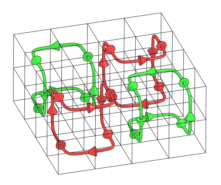
(a) (b)
Figure 7 (a) An example 3D shape S. (b) S split into 4 blocks, each of which can be grown
from its own gene. Note that the surfaces which will be adjacent when the blocks combine will also
be assigned interfaces to ensure correct assembly of S.
(a) (b)
Figure 8 (a) The blocks for the example shape S from Figure 7 with example interfaces
included. (b) View from underneath showing more of the interfaces between blocks. Note that
the actual interfaces created by the algorithm would be shorter, but to make the example more
interesting their sizes have been increased.
in [2]). We will first describe how the shape S can be broken into a set of constituent
blocks, then how the interfaces between blocks are designed, then how individual blocks
self-assemble before being freed to autonomously combine into an assembly of shape S.
5.1 Decomposition into blocks
Since S is a shape in Z3 , it is possible to split it into a set of rectangular prisms whose union
is S. We do so using a simple greedy algorithm which seeks to maximize the size of each
rectangular prism, which we call a block, and we call the full set of blocks B.
After the application of a greedy algorithm to compute an initial set B, we refine it by
splitting some of the blocks as needed to form a binding graph in the form of a tree T such
that every block is connected to at least one adjacent block, but also so that each block
has no more than one connected neighbor in each direction in T . This results in the final set
of blocks that combine to define S, can join along the edges defined by T , and each block
has at most 6 neighbors to which it combines. (Figure 7 shows a simple example.)
5.2 Interface design
The blocks self-assemble individually, then separate from the genome to freely diffuse until
they combine together via interfaces along the surfaces between which there were edges
in the binding tree T . Each interface is assigned a unique length and number. The two
DNA 273:16 Self-Replication
blocks that join along a given interface are assigned complementary patterns of “bumps”
and “dents” and a pair of complementary glues on either side of those patterns (to provide
the necessary binding strength between the blocks). The number assigned to each interface
is represented in binary and the block on one side of an interface has a protruding tile
“bump” in the location of each 1 bit but not in locations of 0 bits, and for the block on
the other side of the interface 1 bits have single tile “dents” where a tile is missing. The
length of each interface dictates which other interfaces have glues at the correct spacing
to allow binding, and the binary pattern of “bumps” and “dents” guarantees that only the
single, correct complementary half can combine with it.
Depending on the shape S and how it is split into blocks, it is possible that there are
too many interfaces of a given length (> 2(n−2)/2 for an interface of length n) to be able
to assign a unique number to each. Our algorithm will attempt to assign a unique length
and number to an interface for all lengths 2 to n/2 (2 being the minimum since there must
be room for the two glues), but since n is the full length of the surface between a pair of
blocks and each bit of the assigned number is represented by a pair of bits, a greater length
can’t be encoded in the tiles along it. Therefore, if there are too many interfaces for a
unique assignment, the shape S is scaled upward. This is repeated until there can be unique
assignments. (Note that there are many ways in which the algorithm could be optimized to
reduce the number of shapes for which scaling is necessary, and/or the amount of scaling,
especially for particular categories of shapes.) More technical details can be found in [2], and
an example of a few interfaces can be seen in Figure 8.
5.3 Block growth
The growth of each block is initiated by a portion of the linear genome called a gene, which
is merely a line of tiles with glues exposed in one direction that encode all of the information
required for the block to self-assemble to the correct dimensions and with the necessary
interfaces. The techniques used to encode the information and allow the blocks to grow
are very standard tile assembly techniques involving binary counters, zig-zag growth patterns,
and rotation of patterns of information. The information to seed the counters and encode the
interfaces is encoded in the outward facing glues of the gene and can be done so with the
universal tile set U since only a constant amount of information needs to be encoded in any
particular gene glue, due to the design of blocks and the fact that each has at most a single
interface on each side which is no longer than that side. Signals are used for detecting
completed growth of blocks, controlling growth of interfaces so “bump” interfaces can’t
complete before all “bumps” are in place, and “dent” interfaces can grow beyond “dent”
locations and then those tiles can fall out, and also so blocks can dissociate from genes.
5.4 Overview of the hierarchical construction
Once a block is freely diffusing and complete, it can combine along its interfaces with
the blocks that have complementary interfaces since, due to the fact that S is a block-
diffusable shape, free blocks can always diffuse into the proper locations to form the complete
shape. We’ve described a tile set U that can be used to (1) form the linear seed assembly
σS , and (2) to self-assemble the blocks which correctly combine to form the target assembly.
The STAM* system TS = (U, σS , 2) will produce an infinite number of copies of terminal
assemblies of shape S (properly scaled if necessary). The only fuel (a.k.a. consumed, junk
assemblies) will be singleton Dent tiles that attached during block growth then detached.
Note that this construction can be combined with the previous constructions as well, to
create a version of a shape self-replicator. Full technical details of the construction, as well
as a discussion of possible enhancements, can be found in [2].A. Alseth, D. Hader, and M. J. Patitz 3:17
References
1 Zachary Abel, Nadia Benbernou, Mirela Damian, Erik Demaine, Martin Demaine, Robin
Flatland, Scott Kominers, and Robert Schweller. Shape replication through self-assembly
and RNase enzymes. In SODA 2010: Proceedings of the Twenty-first Annual ACM-SIAM
Symposium on Discrete Algorithms, Austin, Texas, 2010. Society for Industrial and Applied
Mathematics.
2 Andrew Alseth, Daniel Hader, and Matthew J. Patitz. Self-replication via tile self-assembly
(extended abstract). Technical Report 2105.02914, Computing Research Repository, 2021.
arXiv:2105.02914.
3 Ebbe S. Andersen, Mingdong Dong, Morten M. Nielsen, Kasper Jahn, Ramesh Subramani,
Wael Mamdouh, Monika M. Golas, Bjoern Sander, Holger Stark, Cristiano L. P. Oliveira,
Jan S. Pedersen, Victoria Birkedal, Flemming Besenbacher, Kurt V. Gothelf, and Jorgen
Kjems. Self-assembly of a nanoscale dna box with a controllable lid. Nature, 459(7243):73–76,
May 2009. doi:10.1038/nature07971.
4 Robert D. Barish, Rebecca Schulman, Paul W. K. Rothemund, and Erik Winfree. An
information-bearing seed for nucleating algorithmic self-assembly. Proceedings of the National
Academy of Sciences, 106(15):6054–6059, April 2009. doi:10.1073/pnas.0808736106.
5 Florent Becker, Ivan Rapaport, and Eric Rémila. Self-assembling classes of shapes with a
minimum number of tiles, and in optimal time. In Foundations of Software Technology and
Theoretical Computer Science (FSTTCS), pages 45–56, 2006. doi:10.1007/11944836_7.
6 Florent Becker, Eric Rémila, and Nicolas Schabanel. Time optimal self-assembly for 2d and 3d
shapes: The case of squares and cubes. In Ashish Goel, Friedrich C. Simmel, and Petr Sosík,
editors, DNA, volume 5347 of Lecture Notes in Computer Science, pages 144–155. Springer,
2008. doi:10.1007/978-3-642-03076-5_12.
7 Hieu Bui, Shalin Shah, Reem Mokhtar, Tianqi Song, Sudhanshu Garg, and John Reif. Localized
dna hybridization chain reactions on dna origami. ACS nano, 12(2):1146–1155, 2018.
8 Qi Cheng, Gagan Aggarwal, Michael H. Goldwasser, Ming-Yang Kao, Robert T. Schweller,
and Pablo Moisset de Espanés. Complexities for generalized models of self-assembly. SIAM
Journal on Computing, 34:1493–1515, 2005.
9 Kenneth C Cheung, Erik D Demaine, Jonathan R Bachrach, and Saul Griffith. Programmable
assembly with universally foldable strings (moteins). IEEE Transactions on Robotics, 27(4):718–
729, 2011.
10 Matthew Cook, Yunhui Fu, and Robert T. Schweller. Temperature 1 self-assembly: Determ-
inistic assembly in 3D and probabilistic assembly in 2D. In SODA 2011: Proceedings of the
22nd Annual ACM-SIAM Symposium on Discrete Algorithms. SIAM, 2011.
11 E. D. Demaine, M. L. Demaine, S. P. Fekete, M. J. Patitz, R. T. Schweller, A. Winslow,
and D. Woods. One tile to rule them all: Simulating any tile assembly system with a single
universal tile. In Proceedings of the 41st International Colloquium on Automata, Languages,
and Programming (ICALP 2014), IT University of Copenhagen, Denmark, July 8-11, 2014,
volume 8572 of LNCS, pages 368–379, 2014.
12 Erik D. Demaine, Martin L. Demaine, Sándor P. Fekete, Mashhood Ishaque, Eynat Rafalin,
Robert T. Schweller, and Diane L. Souvaine. Staged self-assembly: nanomanufacture of
arbitrary shapes with O(1) glues. Natural Computing, 7(3):347–370, 2008. doi:10.1007/
s11047-008-9073-0.
13 Erik D. Demaine, Matthew J. Patitz, Trent A. Rogers, Robert T. Schweller, Scott M. Summers,
and Damien Woods. The two-handed assembly model is not intrinsically universal. In 40th
International Colloquium on Automata, Languages and Programming, ICALP 2013, Riga,
Latvia, July 8-12, 2013, Lecture Notes in Computer Science. Springer, 2013.
14 Erik D. Demaine, Matthew J. Patitz, Trent A. Rogers, Robert T. Schweller, Scott M. Summers,
and Damien Woods. The two-handed tile assembly model is not intrinsically universal.
Algorithmica, 74(2):812–850, February 2016. doi:10.1007/s00453-015-9976-y.
DNA 27You can also read