Seismic Performance Assessment of Multiblock Tower Structures as Gravity Energy Storage Systems

Seismic Performance Assessment of
 Multiblock Tower Structures
 as Gravity Energy Storage Systems

 José E. Andrade1 , Ares J. Rosakis2 , Joel P. Conte3 , José I. Restrepo3 , Vahe Gabuchian2 ,
 John M. Harmon1 , Andrés Rodriguez3 , Arpit Nema4 , Andrea R. Pedretti5

 1 Mechanical and Civil Engineering, California Institute of Technology
 2 Graduate Aerospace Laboratories, California Institute of Technology
 3 Department of Structural Engineering, University of California, San Diego
 4 Pacific Earthquake Engineering Research Center, University of California, Berkeley
 5 Energy Vault, Inc., Westlake Village, California

 ABSTRACT
 This paper presents the main findings of a seismic performance assessment for mutiblock tower structures
designed to store renewable energy. To perform our assessment, we deployed in tandem physical and numerical
models that were developed using appropriate scaling for Newtonian systems that interact via frictional contact.
The approach is novel, breaking away from continuum structures where Cauchy scaling and continuum mechanics
are used to model such systems. We show that our discontinuous approach is predictive and consistent. We
demonstrate predictiveness by showing that the numerical models can reproduce with high fidelity the physical
models deployed across two different scales. Consistency is demonstrated by showing that our models can be
seamlessly compared across scales and without regard for whether the model is physical or numerical. The integrated
theoretical-numerical-experimental approach provides a robust framework to study multiblock tower structures and
the results of our seismic performance assessments are promising. These findings may open the door for new
analysis tools in structural mechanics, particularly those applied to gravity energy storage systems.

1 INTRODUCTION
 The world population is expected to reach 10 billion by 2050, necessitating a corresponding increase of 200%
in energy output (UN 2019). At the same time, the US and other nations have goals to reduce CO2 levels by 80%
by 2050 (Markolf et al. 2020). To achieve these massive goals, green energies, such as solar and wind, are being
aggressively pursued to increase the amount of energy available without the negative impact of CO2 production.
The intermittent nature of solar and wind power production, peaks in demand, as well as the need for resilient
infrastructure have created the need for large scale energy storage (Loveless 2012). As of 2019, the US produced
4 × 109 MWh of electricity with only 431 MWh of energy storage available; a seven order of magnitude gap (EIA
2020; Zablocki 2019). It is estimated that the US will require 266 GW of storage for the electric grid by 2030,
up from 176.5 GW in 2017 (IEA 2017). This number is expected to increase to 942 GW by 2040, requiring an
investment in energy storage of $620 billion over the next two decades (Henze 2018).
 Today, electricity storage is dominated by pumped storage hydropower (PSH), furnishing 95% of the large-scale
storage (EERE 2021). One of the appeals of PSH is simplicity: the idea of using gravity to store energy in an uphill
water reservoir when energy is produced and then release it to a downstream reservoir, converting potential energy
into kinetic energy in the process. On the other hand, PSH is limited by topography: there are only so many places
on earth where upstream-downstream reservoir systems can be built. There is clearly a need to find alternative
energy storage systems that share the simplicity of PSH but avoid its limitations. One potentially revolutionary
gravity-driven system is being introduced by Energy Vault (EV), Inc. Figure 1 shows EV’s energy storage concept,
which has been recently proposed and is currently being demonstrated in Switzerland. The proposed idea is to
deploy relatively tall prototype (height, `P ≈ 160 m) multiblock tower structures (MTS) that are connected to
renewable energy sources (e.g., solar, wind), and then use discrete blocks to store energy in the form of potential
energy by lifting the blocks to accrue energy, just like in PSH. Thousands of blocks can be stacked up, as shown
in Figure 1b, each block storing packets of energy that can then be consumed when needed.

 1

a) Energy source/storage b) Energy delivery/storage cycle
 Fully charged Release

 Storage: tower
 Source: solar
 Source: wind

 Accumulation Depleted
Fig. 1. Energy Vault’s gravity energy storage system concept. a) Multiblock tower structures (MTS) proposed to
store renewable energy shown conceptually to be close to green energy sources. b) Energy storage mechanisms for
charging and discharging energy using MTS. An autonomous six-arm crane is used to move blocks as the tower
charges and discharges. In our seismic performance assessment, we focused on the fully charged configuration
shown on the far left.

 The simplicity and promise of the MTS is remarkable, allowing up to 35 MWh of storage per tower anywhere
in the world. The blocks are manufactured using a soil-cement mixture plus other materials from construc-
tion/demolition debris and have a prescribed weight. From a structural mechanics perspective, the novel MTS
concept introduces interesting questions that need to be explored: How can we model such discontinuous structures
both physically and numerically? What are the governing scaling laws that can be used to appropriately design
and deploy physical models across different scales? Particularly relevant is the structural seismic performance of
MTS. In this paper, we take a first step at answering these questions by presenting the results of a year-long
campaign to assess the seismic performance of MTS. We deployed numerical and physical models in tandem, all
against the backdrop of newly-derived scaling laws to achieve not only accurate modeling but also consistency.
Here, we define consistency as the ability to compare physical and virtual models across scales and material prop-
erties. This integrated theoretical-numerical-experimental approach was adopted deliberately since the novel MTS
break away from conventional continuum structures where Cauchy scaling and continuum mechanics provide the
theoretical backbone to model and analyze such systems. Instead, MTS are discontinuous, with discrete blocks
serving as their basic fundamental unit. The discontinuous nature of MTS necessitated a discrete approach to
modeling and analysis, thus requiring a new theoretical backbone fundamentally based on Newtonian mechanics.
The preferred modeling and analysis approach is therefore the discrete element method (DEM) where each block
can be simulated as an individual rigid unit whose interactions are controlled by Newton’s laws and basic frictional
contact mechanics. The numerical models needed complementary physical models at various scales to be properly
validated. At the same time, proper scaling for frictional, multiblock, gravity-driven systems was necessary in
order to design experiments that are representative of the prototype, useful for validation, and can be consistently
compared.
 This paper is the result of a team effort between Caltech, UC San Diego, UC Berkeley, and EV, and is
structured as follows. We first present the modeling campaign methodology to assess the seismic performance
of MTS, with physical and numerical modeling intertwined by proper scaling. The physical modeling campaign
was deployed using shake tables across two different scales: a tabletop scale (1:107) at the California Institute
of Technology (Caltech) and an engineering scale (1:25) at the University of California, Berkeley (UCB). To

 2

appropriately scale from the field prototype to these two modeling scales, we present our scaling methodology with
a key resulting dimensionless number µN (Rosakis et al. 2021) appropriate for such gravitational-frictional systems.
We then present the numerical models, which are furnished using the level set discrete element method (LS-DEM)
(Kawamoto et al. 2016). We focus on the novel features of the LS-DEM, including the process to capture a block’s
morphology as well as the material parameter’s values utilized in our predictions. At the heart of this paper, we
compare the results of the physical and numerical models, which serves as validation of our theoretical approach to
obtain the µN and associated similitude law, as well as validation of our novel numerical models developed using
the LS-DEM. We are pleased to report that the results are encouraging, showing remarkable predictive capabilities
of the LS-DEM models as well as robust consistency across scales and models. Finally, we close the paper with
some discussion on our findings and their significance for gravity-driven storage of renewable energy.

2 METHODOLOGY: SIMILITUDE, PHYSICAL AND NUMERICAL MODELING
 The main goal of our campaign is to validate the computational (virtual) models of EV’s MTS using appropriate
physical models across scales, as shown in Figure 2. To this end, two major tasks need to be undertaken: 1)
development of appropriate physical models M1,2 of MTS at various scales, and 2) development of virtual models
V1,2 of MTS. Direct comparison with the prototype is not yet feasible; there are no full-scale operational MTS
at this time, hence the importance and relevance of appropriate physical models to enable comparisons, i.e. V1
vs. M1 and V2 vs. M2 . We adopt the definition of physical model given by (Janney et al. 1970): “A structural
model is any structural element or assembly of structural elements built to a reduced scale (in comparison with
full size structures) which is to be tested, and for which laws of similitude must be employed to interpret test
results”. To be feasible and effective, physical models are scaled relative to the prototype. This scaling requires
an immediate choice of geometry, material and loading (e.g., input ground motion record) for the physical model,
hinging crucially on similitude. At the same time, similitude requirements are furnished by the derivation of
dimensionless numbers (i.e., Π-groups), which can be shown to control the physical system regardless of choice
of basic dimensions, e.g., length, time, and mass. The choice of dimensionless numbers, which is the subject of
an accompanying paper (Rosakis et al. 2021), drives the design of the physical models and the applied dynamic
loading.
 We designed and constructed the physical models as defined in (Harris and Sabnis 1999): geometrically similar
to the prototype in all respects, including the dynamic loads, furnished by shaking tables. As shown in Figure 2, two
physical modeling campaigns were devised and conducted: one at Caltech at 1:107, and another at UCB at 1:25.
Below, we present some of the details of such direct dynamic models and how we achieved similitude across these
different scales. Suffice it to say, using the Buckingham’s Pi Theorem (BPT), we obtained Π−groups, required to
be invariant between prototype and model. One such Π-group is Π1 := µN , a non-dimensional number as mentioned
above and elaborated below. It turns out that µN is similar to the well-known Froude number FrN . Incidentally,
for dynamic similitude of civil engineering structures, the most commonly used non-dimensional numbers are the
Cauchy number C N , used when elasticity controls the response behavior of the system; and the Froude number
FrN , used for appropriately scaling hydraulic and frictionless structural systems where gravitational loading is
important (Moncarz and Krawinkler 1981). To our knowledge, no non-dimensional number has been previously
proposed to properly scale the dynamic behavior of multiblock systems whose nonlinear dynamic response is
controlled by gravitational and frictional restoring forces.
 Armed with the µN to properly scale our MTS dynamic (physical) models, we designed a combined theoretical-
numerical-experimental campaign whose methodology and key results we present in this paper. Figure 3 shows
an overview of the campaign, including the physical models (specimens) developed, as well as the virtual models
deployed. It is important to highlight that this was a unique exercise in which theory and modeling were deployed
in tandem to analyze the MTS. The numerical models were deployed first since these could readily explore ideas
for theory and experiment. However, it was not until the theory and physical models came about that a deep
understanding and validation of the numerical model were achieved. Below, we describe our efforts in validating
the numerical models and in the process we describe the multiscale physical modeling campaign and then the
intricacies of the numerical model used. Much like the theory and physical models, the numerical model had to
represent the MTS accurately: capturing the block geometry, simulating the frictional contact interfaces, properly
transmitting dynamical loading, and scaling to the thousands of blocks involved in the virtual and physical models.
As shown in Figure 3, complete consistency was imposed across all models, making it possible to compare M1
with V1 , M2 with V2 , but also, and most importantly, being able to analyze all results across models M1,2 ,
and V1,2 consistently. The virtual model also enables us to show consistency: comparing the correctness of the

 3

a) Validation at 1:107 scale b) Validation at 1:25 scale

 Physical model [M2] Virtual model [V2]

 Physical model [M1] Virtual model [V1]

 Validate Validate
 M 1 ≡ V1 M 2 ≡ V2
 [View A1] [View A2]

 Base Base

 Base Base

 Scaled ground motion c) Scaling system physics Scaled ground motion
 Similitude validation
 M 1 ≡ M 2 V 1 ≡ V2

Fig. 2. Schematic representation of combined theoretical-physical-numerical modeling campaign deployed for
MTS. Physical dynamic models were compared with virtual models of MTS. a) Validation at 1:107 scale comparing
physical dynamic model M1 to virtual LS-DEM model V1 . b) Validation at 1:25 scale comparing physical dynamic
model M2 to virtual LS-DEM model V2 . c) Appropriately scaled input ground motions, achieved by imposing
similitude requirements.

similitude theory at levels of accuracy that are superior to the physical models. In what follows, we describe in
detail the development of physical and virtual models for MTS, as well as the most salient results obtained with
such consistent models.

3 PHYSICAL MODELING
 The physical models developed herein are needed to experimentally study the nonlinear behavior of MTS
subjected to input ground motions. The purpose of such experiments is the validation of our newly developed
virtual models, to be presented in the next subsection. To be useful, a physical model should be able to predict
the nonlinear dynamic response of the MTS prototype. This necessitates similitude across scales, materials,
loading, and instrumentation (diagnostics). In this section, we explain how we achieve similitude and, hence,
predictiveness in our physical models. We focus on dynamic modeling theory (DMT), encompassing similitude
requirements, geometric and material properties, and dynamic loads. We also explain our approach to multiscale
model construction and diagnostics.
 Our starting point is dynamic modeling theory (Moncarz and Krawinkler 1981). Perhaps the most funda-
mental component of DMT is dimensional analysis, which is built around the Buckingham’s Pi Theorem (BPT)
(Buckingham 1914) and the concept of similitude. The dynamic behavior of a physical system, such as the MTS

 4

Wood Metal Concrete Virtual
 = 1.51 m = 1.51 m = 6.46 m = any

Fig. 3. Overview of experimental campaign showing physical models used with different geometries and materials
(e.g., wood, metal, concrete). Virtual models were set up block-by-block with the same geometric and material
properties, enabling direct comparison. Bottom row shows blocks as fundamental units of MTS. Notice that
physical blocks were marked to enhance kinematics tracking via digital image correlation (DIC). Bottom right
shows details of the virtual block, which is defined using level sets, requiring a grid of points were the level set
function is defined. Validation necessitates complete consistency between all models: physical and virtual. Every
tower consists of 38 stories or layers with 188 blocks each, for a total of 7,144 blocks. The pattern of each layer is
shown in the top view (top row) with each layer alternating the pattern by 90 degrees.

we are interested in, can be said to be controlled by a dimensionally homogeneous function such that

 f (v; a; `; µg; ρ) = 0 (1)

where the arguments of the (implicit) function f are physical quantities believed to be relevant to the MTS
behavior. In the case of MTS systems, we assume the towers are composed of rigid blocks whose behavior is
controlled by Newtonian mechanics and frictional contact restoring forces, with five main physical quantities of
interest. The quantities of interest take the form of physical variables such as velocity v and acceleration a,

 5

geometrical parameters such as the height of the tower ` (see Figure 3), material system parameters such as
the friction coefficient µ and the mass density ρ, as well as the gravitational acceleration g. We point out that
Equation (1) is a modeling choice, as per usual in the application of BPT. At the same time, there are three basic
units in these systems, i.e., length, time, and mass.
 The BPT states that the dimensional homogenous function f can be rewritten as a non-dimensionally homo-
geneous function with two non-dimensional variables, or Π-groups, so that

 F (Π1 ; Π2 ) = 0 (2)
 √ √ √
where in this case, Π1 := µN = v/ `µg = FrN / µ and Π2 := a/µg. We note that FrN := v/ `g is known as the
Froude number, a typical dimensionless group used in frictionless gravity-controlled systems. The presence of
the inter-block friction coefficient µ next to the gravitational acceleration g in the denominator of both Π-groups
highlights the frictional-gravitational nature of the MTS (Rosakis et al. 2021). Similitude requires invariance in
Π-groups across scales in general and in particular between model (M) and the prototype (P) so that ΠM P
 1 = Π1 and
 M P
Π2 = Π2 . Hence, according to DMT, two systems or models are similar if their Π-groups are equal. Interestingly,
for rigid-block systems, the material density does not appear in the Π-groups and consequently is not a physical
variable as will be corroborated experimentally (Gabuchian et al. 2021). Further, one can choose three scales in
this problem. We choose (for modeling convenience) the following scales between model (M) and prototype (P):
the length scale λ` := `M /`P , the gravity scale λg := g M /g P , and the frictional scale λµ := µM /µP . In the modeling
results presented herein, we chose λ` = {1/107, 1/25}, λg = 1 and λµ ≈ 1. The former corresponding to the length
scales used in the lab at Caltech and UCB, respectively. The latter two corresponding to the same gravitational
field and similar coefficient of friction in the materials used for the unit blocks shown in Figure 3. Finally, it then
follows that the kinematic variables scale such that
 p
 v M = v P λ` λµ λg ≈ v P λ`
 p

 aM = aP λµ λg ≈ aP (3)
 s
 M P λ` p
 t =t ≈ tP λ`
 λµ λg

since λµ λg ≈ 1 for the results presented herein. These scaling relations were used in the construction, excitation
and instrumentation of the experiments conducted at the tabletop and engineering scales and described next.
3.1 Tabletop Scale Models (λ` = 1/107)
 This set of experiments was performed at the California Institute of Technology. The details of this portion
of the physical modeling campaign are specified in an upcoming publication (Gabuchian et al. 2021). Figure 4a
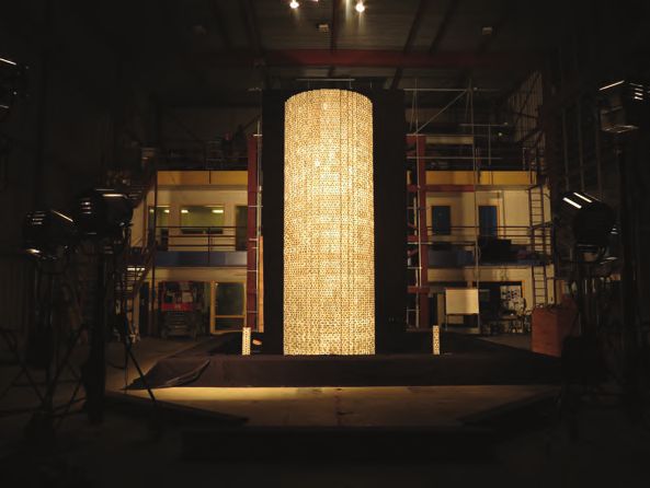
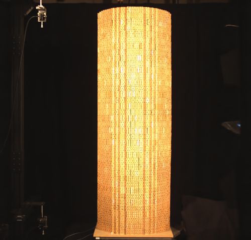
shows a detailed picture of the experimental layout at this scale. The main dimension of the tower is `M1 = 1.51 m
(Fig. 4a), with corresponding basic block dimensions of `M 1
 0 = 4 cm (Fig. 3). The blocks used were made out of
wood and metal (aluminum). In this paper, we focus exclusively on the wood towers and will report the results
on the metal tower in a future publication showcasing the experimental campaign at Caltech in detail (Gabuchian
et al. 2021). Unlike the aluminum blocks, wood blocks have friction coefficients similar to those of concrete and
hence λµ ≈ 1, and the experiments were conducted under full gravitational acceleration, i.e., λg = 1. Hence, the
only major difference between the models and prototype is the length scaling λ` .
 In this paper, we will showcase the results of a test on a wood tower that experiences the 2019 Mw = 7.1
Ridgecrest earthquake because of its relevant location to solar and wind farms in California. We simulate the
velocity time history of the strong motion as recorded at China Lake station 3.5 km away from the fault line.
The shake table at Caltech has one-dimensional horizontal capabilities so we select the strongest ground motion
component (360 degree channel) for our physical simulation. The one-dimensional shaking is simulated by actuating
the shake table platen along the axis parallel to the plane of view of camera A shown in Figure 4. The velocity
record to be inputed in the shake table controller is scaled according to the scaling relations specified in Equation (3)
and depicted at the bottom of Figure 2c. The implication of the scaling is an input velocity record whose speed
and time are one order of magnitude slower and shorter than in the prototype (real scale). This scaling guarantees
similarity between prototype (P) and model (M1 ).
 A significant challenge was the construction of model towers at different scales. To simulate the layered pattern
used in the prototype and furnished by a six-arm crane (see Fig. 1), we use a carrousel or stencil with rectangular
holes corresponding to the cross sectional dimensions of the basic blocks (Gabuchian et al. 2021). The carrousel

 6

a) Laboratory: ` = 1/107 b) Laboratory: ` = 1/25

 Lights (top) CAM B Lights (top) CAM B

 = 1.51 m
 = 6.46 m

 Lights (left) Lights (right) Lights (left) Lights (right)
 Laser velocimeters Base
 Cameras Photo off CAM A axis Cameras Base Photo off CAM A axis

 d) High-speed photography c) Multiscale experimental layout e) Laser velocimeters
 and accelerometers
 Raw Correlated Lights (top) CAM B
 Base
CAM B (top)

 Laser velocimeters Laser beam
 and accelerometers

 Accelerometers f) Accelerometers
CAM A (front)

 Lights (left)

 Base
 Lights (right)

 CAM A Ground motion input

Fig. 4. General layout of physical models at a) Caltech (λ` = 1/107), and b) UCB (λ` = 1/25). c) Schematic
of the experimental layout with the model centered on top of the shake table platen, whose motion is observed
by two cameras procuring high-speed photographs in real time, and additional instrumentation consists of laser
velocimeters and accelerometers. d) Typical snapshots produced by high-speed photography and digital image
correlation. e) Closeup of laser velocimeters and accelerometers. f) Accelerometer array on the back of towers at
UCB.

effectively furnishes a template that provides the location of each of the 188 unit blocks that constitute a single
story in the tower (see Fig. 3). Once a story is placed, the carrousel is lifted and then rotated 90 degrees to furnish
the template for the next story. This process is repeated 38 times to provide the exact location of each of the
38 × 188 = 7, 144 blocks in each tower. Both the tiling pattern and juxtaposition of the stories are important to
the stability of the tower as they influence the level of frictional confinement at the top and bottom of each block.

 7

As for the diagnostics, we chose full-field optical methods at this scale for these main reasons: 1) the ability of
optical methods to scale up, 2) the ability to take contactless measurements, which was very important to streamline
model construction, especially at this scale, and 3) the ability to obtain transient field quantities of interest such
as kinematics and deformations. As shown in Figure 4, two high-speed cameras are placed in front and on top of
the tower models. A typical camera view is shown at the bottom left of Figure 4. We utilized the method of digital
image correlation (Sutton et al. 2009; Gabuchian et al. 2021) to convert incremental displacements of the unit
blocks into strain fields. In this way, we obtain sub-block resolution kinematic field time histories (displacement,
velocity, acceleration) and corresponding strain field for each model tower. We believe that the use of kinematic
and deformation fields for structural mechanics is novel and quite promising as highlighted in our results. To verify
our results, we also deployed three laser velocimeters: one at the platen level, one at the first level and the other
at the top of the tower. These velocimeters enabled us to capture the particle velocities of discrete locations (at
very high temporal resolution) in the tower specimen as a function of time and compare them to the velocity field
evolutions obtained by our full-field optical measurements at those locations.
 As we will describe in the next subsection, our process is amenable to upscaling, necessitating minimal adap-
tation and compatibility between scales. In other words, the procedures used to model MTS at the tabletop scale
λ` = 1/107 are fully compatible and form-identical to the process used to model MTS at the engineering scale
λ` = 1/25.
3.2 Engineering Scale Models (λ` = 1/25)
 This set of experiments was performed at the UCB Earthquake Simulator Laboratory, currently the largest
six-degree-of-freedom shaking table in the United States. The details of this portion of the physical modeling
campaign are specified in an upcoming publication (Restrepo et al. 2021). Figure 4b shows a detailed picture
of the experimental layout at this scale. The main dimension of the tower is `M2 = 6.46 m (Fig. 4b), with
corresponding block dimensions of `M 2
 0 = 17 cm (Fig. 3). The basic blocks are made out of concrete, so there
is direct material similarity with the prototype, i.e., λµ = 1. Also, just like in the previous subsection, the
experiments were conducted at full gravity, i.e., λg = 1. Therefore, once again, the only dimensional scale that has
major influence is the length scale λ` = 1/25.
 Similar to the tabletop experiments, we showcase the results of the concrete tower at engineering scale (λ` =
1/25) for the 2019 Mw = 7.1 Ridgecrest earthquake. We take the same record as before, from a station located
3.5 km away from the fault line. Unlike the Caltech small shake table, the UCB shake table is capable of
imposing three-dimensional translations and rotations. Hence, we simulate the velocity time history in all three
displacement axes, as depicted in Figure 2b. The 3D shaking is simulated by actuating the shake table platen
along the recorded north-south and east-west directions and also in the vertical direction, which corresponds to
the longitudinal dimension of the tower (see Fig. 2b). Consistent with DMT, the 3D acceleration record inputed
in the shake table controller is scaled according to the relations specified in Equation (3). There are two major
differences with respect to the seismic simulation in the Caltech tabletop experiments. First, even though the
input earthquake record is technically the same, the 3D nature of the record at the UC Berkeley shake table is
much more realistic than the single-axis input at Caltech. Second, the velocity and time scalings used at the
engineering scale model (M2 ) are about a fifth of those of the prototype (P), in other words, v M2 ≈ 2v M1 ≈ 1/5v P
and tM2 ≈ 2tM1 ≈ 1/5tP as dictated by scaling.
 Similar to the material, geometry and excitation, the construction process was multiscale, allowing towers to
be built using the same general technique relying on a carrousel or stencil. The same pattern of the blocks at each
floor was obtained, with 188 blocks per layer (see Fig. 3). However, a significant difference from the smaller scale
was the need to use a crane to support, lift, rotate and align the stencil–essential operations to build towers in
the specified layered pattern. The layering process was repeated 38 times (number of stories in the tower), with a
total of 7,144 concrete blocks per tower. Needless to say, building towers of height equivalent to that of a two-story
building is a multi-day operation with a dedicated building crew. The specifics of the tower construction at the
UCB shake table are provided in an upcoming publication (Restrepo et al. 2021).
 Finally, the same optical diagnostics concept was used for the engineering scale towers: high-speed photography
as the basis for digital image correlation to obtain sub-block resolution kinematics. As shown in Figure 4b, two
cameras were positioned to capture the kinematics of the concrete towers. Camera A, positioned to observe the
front plane of the tower and coaxial with the horizontal velocity v1M2 and the vertical velocity v3M2 (see Fig. 2b).
Camera B, positioned to observe a top plane of the tower and coaxial with the horizontal velocities v1M2 and
v2M2 (see Fig. 2b). To verify the kinematics obtained using optical measurements combined with DIC, classical

 8

accelerometers were installed on the back of the tower as shown in Figure 4. The array of accelerometers was
installed along the center of the tower and was distributed over the height of the tower. The measurements
obtained using high speed photography combined with DIC match the measurements obtained with point-wise
via velocimeters (in tabletop experiments) and the accelerometer array. This verification provides confidence to
our optical measurements, which as indicated before are quite novel to structural diagnostics, especially at the
engineering scale. The advantages of optical measurements have been outlined in the previous subsection, but here
we should emphasize that scalability is massive at the engineering scale: the effort to setup high-speed cameras
and lights is comparable across scales, whereas the installation of analog measurements, such as accelerometers,
scales with the number of sensors and the model dimensions.
 The physical models at tabletop scale (λ` = 1/107) and engineering scale (λ` = 1/25) are similar due to their
grounding on the dynamic modeling theory (DMT) outlined in (Rosakis et al. 2021). These similar physical models
provide a wealth of data showcasing the dynamic behavior of MTS. These data are relevant and invaluable in the
validation of numerical (virtual) models, which are presented in the next subsection.

4 NUMERICAL (VIRTUAL) MODELING
 The virtual models in this campaign are needed to show predictive capability to the physical models at both
scales. The key to achieving this goal for MTS is in the kinematics of the blocks, not their deformation, so a
model that focuses on the efficient modeling of contact and rigid body motion is ideal. Continuum modeling
does not achieve this so we have opted for a discrete approach. With this in mind, the level set discrete element
method (LS-DEM) was a natural choice as a modeling technique. Discrete element methods rely on the rigid body
assumption and Newton’s laws to accurately and efficiently model the contact kinetics and individual kinematics
of the discrete elements of the system. In this way key information such as contact forces, frictional dissipation,
and the motion of each block over time can be readily and efficiently studied for towers composed of thousands
of blocks. The level set variant of DEM is used as a way to define the shape of the blocks without limitations
(Kawamoto et al. 2016). Blocks in this study are limited to the simple block shape, however, validating the level
set variant now enables the study of more exotic geometries in the future.
 In LS-DEM, particle geometry is defined using both level set functions and a set of discrete surface points
that work together in a contact algorithm described in full by (Kawamoto et al. 2016). Level sets are functions
that take a position in space as input and then output the signed distance of that position to an object surface
where outside an object is positive and inside is negative. Thus if a surface point position for particle i, pi , gives
a negative level set value from the level set of particle j, φj (x), then particle i and j are in contact. The level
set value is called the overlap and is denoted as d, and the level set also provides the contact normal direction n̂
through the gradient.
 φj (pi ) = d (4)
 ∇φj (pi )
 = n̂ (5)
 |∇φj (pi )|
In the bottom right of Figure 3, a visualization produced from the level set of the representative block is shown
with the surface points overlayed.
 Once contact is established, the contact forces and the resulting moments are calculated using a contact law.
No contact law is specific to the model and for this study a linear force-displacement relationship is used for both
normal and shear forces. For the linear model, normal and shear forces are written as

 F n = kn dn̂ + cv rel
 n (6)

 ∆F s = ks v rel
 s ∆t (7)
where v rel
 n and v s
 rel are the relative velocity between the contact point on each of two colliding blocks in the

normal and shear direction, respectively, ∆t is the time step, kn and ks are the normal and shear stiffnesses,
and c is the contact damping. The contact damping is used to model inelastic contact and is controlled by the
non-dimensional coefficient of restitution, cres . The shear force uses an incremental approach due to the history
dependent nature of friction. Coulomb friction is used to model the maximum frictional force as

 Fsmax = µ||F n || (8)

 9

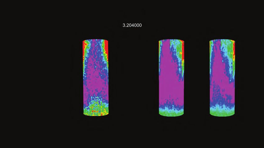
Parameter Wood Concrete Units
 Normal Stiffness (kn ) 30 1,050 MN/m
 Shear Stiffness (ks ) 26 1,000 MN/m
 Density (ρ) 800 2,320 kg/m3
 Friction Coefficient (µ) 0.63 0.59 none
 Coefficient of Restitution (cres ) 0.3 0.5 none
 Block Height Std. Deviation (σH ) 0.155 0.5 mm

 TABLE 1. Complete list of parameters used in numerical modeling.

Moments can then be calculated using the forces and the center of mass of the particle, xm ,

 M = (pi − xm ) × F (9)

With the forces and moments from the forces calculated, the motion of the particles can then be determined by
Newton’s Second Law and kinematics, which results in new contacts and the process iterates.
 The contact algorithm requires certain physical parameters that can all be determined from measurements on
individual blocks without the need of tower construction, and are reported in Table 1. All parameters in this
study were measured at the appropriate scale and for the particular choice of material. It should be noted that
parameters could also be determined through scaling, but this was not pursued in this study. These parameters
are common for all applications of DEM except for the application specific parameter, block height variation. This
parameter was added after observations from the physical models showed that variation of block heights were
causing imperfect stacking arrangements which were believed to affect the dynamics of MTS. The model uses an
explicit time integration scheme in which the time step can be set to a known critical time step (Tu and Andrade
2008).
 The ground is modeled as a flat plane that develops contact with blocks when a block’s surface points cross
that plane. Ground motion is modeled by prescribing the motion of the plane. The imposed earthquake ground
motion record is often recorded at a different sampling rate than the numerical simulation time step and therefore
linear interpolation is used to up-sample the applied base motion.
 Models of the MTS were initialized with each block placed exactly in their designed location in the lateral
directions, but in the vertical direction some space was added in between the block layers. The fictitious initial
vertical separation is to allow the tower to find equilibrium naturally with gravity and without the interference of
initial contact forces. Tower layers are added one at a time and each layer is lowered at a set velocity to replicate as
closely as possible how the tower is built experimentally. This process of the tower settling into static equilibrium
is completed before any earthquake ground motion is applied. In cases where there is significant block height
variation, a damping procedure is recommended to achieve the target tower quality that will be discussed in a
future paper on the subject.

5 RESULTS AND MODEL COMPARISONS
 In this section, we showcase the most salient results obtained from the physical models M1 and M2 , and
the virtual models V1 and V2 . As mentioned earlier, our main objective here is to validate the virtual models
using appropriately-scaled physical models. Hence, as shown in Figures 5 and 6, we will compare the predictions
obtained from V1 of the response obtained in M1 at the tabletop scale (λ` = 1/107), and the predictions obtained
from V2 of the response obtained in M2 at the engineering scale (λ` = 1/25). In addition to validating the virtual
models against physical models, we also present results related to the validity of the physical models, namely:
verify the kinematic fields obtained from the high-speed cameras and DIC against the independent point-wise
measurements obtained using velocimeters and accelerometers; ascertain the consistency of µN and therefore the
similarity between models at different scales (e.g., V1 ≡ V2 ; M1 ≡ M2 ). Hence, we will show that 1) our virtual
models are valid, by comparing them with 2) valid field measurements using DIC, and we will show that 3) the
whole dynamic modeling approach is consistent.
 Figure 5 shows results comparing the virtual model V1 with measurements from physical model M1 at the
tabletop scale. The left-hand side of the figure shows comparisons of the v1 component of velocity at three different
time-stations t1 , t2 , t3 . The component v1 corresponds to the most significant motion in the models since, in the
physical model at λ` = 1/107, the strong ground motion is aligned with that direction. In fact, the right-hand side

 10

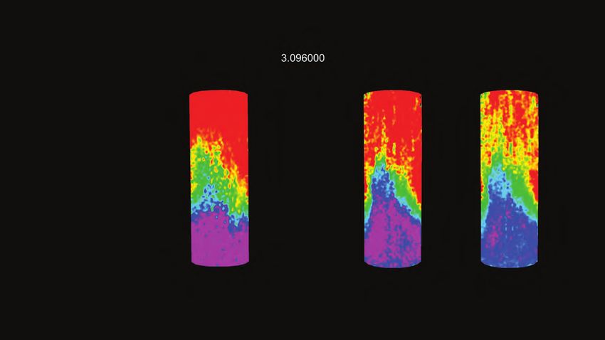
a) Tower response: v1 field, ` = 1/107, Ridgecrest 1D b) Spine records: v1 (black & red dots)

 5 cm/s Measurement
 Prediction
 37
Experimental measurement

 35
 33
 31
 29
 27

 1.51 m
 v1 (cm/s)
 1.5 -1.5

 11
LS-DEM prediction

 9
 7
 5
 3
 1
 Base

 t1 = 0.71650 s t2 = 0.73520 s t3 = 1.00400 s 0.5 t1t2 t3 = 1.00400 t (s)

Fig. 5. Overall results and comparisons between physical (M1 ) and virtual (V1 ) models at λ` = 1/107 scale. a)
Snapshots at three different time stations comparing velocity field v1 for (top) physical model M1 with (bottom)
virtual model V1 . b) Velocity v1 time history for physical model M1 and virtual model V1 at different height levels
(points sampled in a)). Shadow band around virtual model predictions V1 shows spread for 10 different realizations
of virtual tower configurations accounting for random block height variability. Thick (red) line corresponds to V1
prediction average.

panel of Figure 5 shows the time history of the component v1 of velocity in the virtual and physical models at
various stations along on height of the tower. The time history shown at the bottom corresponds to the motion at
the base of the physical model M1 , which is used as input for the virtual model V1 . Before we analyze the results
in more detail, it should be remarked that the virtual model V1 was run ten times, each time corresponding to a
realization of a tower composed of blocks of slightly different heights `0 . The details pertaining to such models will

 11

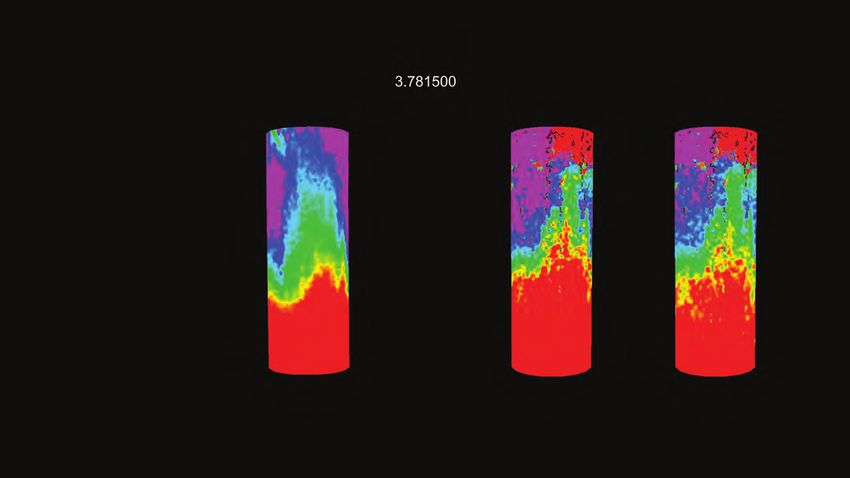
be published in an upcoming paper (Harmon et al. 2021). We chose a normal distribution for the block’s height,
with a standard deviation of 0.155 mm (see Table 1) obtained from measurements taken from the wood blocks used
in the construction of the physical tower at the tabletop scale. Interestingly, without the inclusion of these small
imperfections, the virtual model predictions are not as accurate as those obtained using variable block heights.
Now, we turn our attention to analyzing the results shown in Figure 5 both qualitatively and quantitatively.
 It is worth noting that the v1 velocity fields from the experimental and virtual tower specimens in Figure 5a
are plotted at the same time stations and using the same intensity map. The qualitative similarity in the velocity
fields is strong. Even more remarkable, however, is the quantitative agreement in the details and morphology of
the velocity maps. In both models, one can observe a velocity front, which moves upwards from the base to the
top of the tower at the 38th story. This movement can be observed in both models shown in Figure 5a by looking
at the velocity fronts at the three different time stations shown. The timing, location and morphology of the
v1 velocity field in both models are in very good agreement, demonstrating the accuracy of the virtual model at
this scale λ` = 1/107 using wood blocks. Looking more deeply, Figure 5b shows the time history comparisons for
v1 obtained in both models. Unlike the spatially continuous snapshots in time shown on the left sub-figure, the
continuous time histories show the evolution of v1 at discrete locations (red and black points) along the height of
the model towers. The agreement between the predictions and measurements is excellent, with the virtual model
faithfully capturing the nonlinear response time history along the height of the tower. In a way, Figures 5a,b
offer two sides of the same coin, with one panel (a) offering continuous fields in space but discontinuous snapshots
in time, and the other panel (b) showing continuous time histories but at discontinuous locations in space. The
picture painted by both views is consistent: the virtual model V1 accurately predicts the measured data obtained
from the physical model M1 .
 Figure 6 shows results for the engineering scale models λ` = 1/25. Once again, the virtual models were run ten
times with variable block heights corresponding to a normal distribution with standard deviation of 0.5 mm (see
Table 1) obtained from measurements of many concrete blocks in situ. The shaded band in Figure 6b corresponds
to the fan of results obtained from the 10 different realizations of the virtual model V2 . Accounting for randomly
variable height `0 was crucial for obtaining accurate predictive results as in the tabletop case. Figure 6a shows
comparisons of the velocity v1 field for both physical model M2 and virtual model V2 at three different time
stations t1 , t2 , t3 . In contrast to the tabletop experiments, the engineering scale models at λ` = 1/25 are subjected
to three dimensional input motion at the base (see Figure 2b). Nevertheless, the component v1 corresponds to the
strongest recorded direction of motion and hence presents a relevant component of the velocity field for purposes
of model validation. As shown in Figure 6a, the velocity fields predicted using the virtual model V2 compare
remarkably well to the velocity fields measured from the physical model M2 . As in the tabletop models, one can
observe a velocity front whose location, temporal evolution and shape is similar in both models whose results are
plotted using the same color map. The qualitative and quantitative similarities in the velocity fields is remarkable
and complemented by the results showing the velocity time histories.
 Figure 6b shows the v1 velocity time histories for the virtual and physical models at discrete locations along
the height of the towers. The v1 time histories for both V2 and M2 compare well, with the salient features in the
measured signals being captured by the virtual model. The high and low frequency components of response are
well predicted and the peaks and valleys in the time histories correspond to a high degree of accuracy. Figures 6a,b
show complementary sides of the measured and predicted responses and indicate a high predictive capability of
the virtual model. It is also important to note that there is no deterioration in the predictive power of the virtual
model as the length scale is increased; there is also an important level of consistency in the physical models even
though the nature of the imposed base excitation differed in dimensionality (1D vs. 3D).
 This brings us to the issue of consistency. While it is clear that the virtual and physical models are comparable
at each scale, i.e., V1 ≡ M1 and V2 ≡ M2 , it is not clear if models are consistent across scales, namely V1 ≡ V2 and
M1 ≡ M2 . Consistency requires complete similarity between models and scales, provided the input motions are
also similar. In the results presented herein, there is not complete consistency since the dimensionality of the base
excitation is not consistent. However, we did perform simulations using virtual models with consistent excitations
and found that these models are fully consistent. Similarly, we performed simulations using physical models that
are fully consistent across scales and find that these models are indeed consistent. We present the details of these
findings in (Rosakis et al. 2021; Harmon et al. 2021), but report here that the models are fully consistent due to
their appropriate similarity predicated on µN .
 Finally, we also report on the validity of the optical measurements used in the results provided in Figures 5 and
6. How do we know that the measured kinematics and subsequently calculated fields using DIC are accurate? To

 12

a) Tower response: v1 field, ` = 1/25, Ridgecrest 3D b) Spine records: v1 (black & red dots)

 10 cm/s Measurement
 Prediction
 37
Experimental measurement

 35
 33
 31
 29
 27

 6.46 m
 v1 (cm/s)
 3.0 -3.0

 11
LS-DEM prediction

 9
 7
 5
 3
 1
 Base

 t1 = 3.1240 s t2 = 3.2320 s t3 = 3.8095 s 3 t1 t2 t3 4 t (s)

Fig. 6. Overall results and comparisons between physical (M2 ) and virtual (V2 ) models at λ` = 1/25 scale. a)
Snapshots at three different time stations comparing velocity field v1 for (top) physical model M2 with (bottom)
virtual model V2 . b) Velocity v1 time history for physical model M2 and virtual model V2 at different height levels
(points shown on a)). Shadow band around virtual model predictions V1 shows spread for 10 different realizations
of virtual tower configurations accounting for random block height variability. Thick (red) line corresponds to V2
prediction average.

assess this important question, we have to verify the optical measurements using independent measurements and
evaluate their consistency. In the case of the results shown in Figure 5, the optical measurements are compared
with velocimeter data (not shown) obtained at the base, bottom and the top of the tower. In other words, the time
history shown for the base, block 1 and block 37 are compared with velocimeter data obtained at those locations.
While the data and comparisons will be published in a subsequent publication (Gabuchian et al. 2021), we can

 13

report that the time histories coincide to within the accuracy of the measurement methods. Hence, the data at
λ` = 1/107 has been validated. We used the same optical technique for the experiments at the engineering scale
λ` = 1/25. In the case of the engineering scale measurements, however, we had access to a larger number of locations
on the tower where acceleration measurements were taken. As shown in Figure 4, an array of accelerometers was
installed along the height of the tower to provide indirect validation of the optical measurements. The validation
is indirect since the accelerometers are placed on the back of the tower, while the optical measurements are taken
on the front of the tower. However, there is a relatively high degree of symmetry in the problem (especially
early on during the seismic tests) and hence comparisons can be made. We report on the data and comparisons
of the optical and accelerometer data in an upcoming publication (Restrepo et al. 2021). We also report here
that the optical and accelerometer data obtained are in very good agreement. Also, the velocities obtained at
the base of the tower are compared with those reported by the control system of the shake table at UCB and
they match reasonably well. A number of independent measurements coincide in space and time with the optical
measurements; we therefore conclude that the optical measurements are valid across scales.

6 CLOSURE
 We have presented a systematic methodology to assess the seismic performance of a new type of multiblock
tower structure (MTS) designed to serve as gravitational energy storage systems. These MTS possess great
potential as energy storage systems at a moment when there is much interest and need to expand energy storage
capacity worldwide. The discontinuous nature of the MTS systems pose a number of challenging and interesting
engineering questions, particularly, how can we model such discontinuous gravitational-frictional systems? This
paper summarizes a year-long integrated theoretical-numerical-experimental campaign to begin answering the
question of modeling such systems. The presentation is rather superficial and incomplete due to the nature of this
introductory paper. However, we have reported on a number of important findings that will be expanded in a
number of companion publications (Rosakis et al. 2021; Harmon et al. 2021; Gabuchian et al. 2021; Restrepo et al.
2021). In particular, we have shown the process by which we have constructed similar models of MTS across scales
λ` = 1/107 and λ` = 1/25 and used them to validate virtual numerical models using the level set discrete element
method (LS-DEM). The central piece to achieving similar physical models is the non-dimensional number µN ,
which seems to control gravitational-frictional systems. This new non-dimensional number expands the toolbox
of experimental dynamic modelers used to continuum classical numbers such as Cauchy and Froude, useful in
modeling elastic and frictionless-gravitational systems, respectively, in engineering.
 Appropriate scaling enabled us to successfully design, build and diagnose MTS under dynamic loading. We
utilized the same methodology regardless of scale, particularly in construction and diagnostics. The diagnostics
deployed a novel and scalable concept of optical measurements hinging on high-speed photography enhanced with
DIC. This enabled the measurement of kinematic fields at sub-block resolution, furnishing spatiotemporal fields
for displacement, velocity and acceleration. The optical measurements were properly validated using a number of
independent measurements across material, length and time scales.
 The main objective of the study was to validate computational (virtual) models of MTS which are predicated
on Newtonian Mechanics, a significantly different framework from finite element modeling, which is rooted in
continuum mechanics. Our discontinuous approach uses basic physics and contact-frictional mechanics to model
MTS as a collection of rigid blocks that interact with each other, being controlled by Newton’s Second Law and
modulated by contact-frictional mechanics. This simple physics-based approach was shown to be predictive in
space and time, regardless of length scaling. Strong similarities in fields and time histories of velocity components
were shown as salient examples of a wealth of results that will be subsequently reported.
 The results presented in this paper show that discrete models, such as LS-DEM, can be appropriately used to
simulate the behavior of complex MTS. We have also shown that dynamic modeling theory provides the tools to
construct and test similar physical models of MTS. Equipped with these predictive and validated modeling tools,
one can perform analysis of MTS for a broad range of expected seismic loads across the globe. It is anticipated
that such an approach can be used to design future MTS systems and, eventually, assess the seismic performance
of these novel gravity energy storage systems.

7 ACKNOWLEDGEMENTS
 This research was supported by Energy Vault, Inc. We gratefully acknowledge EV’s support, encouragement
and freedom during this project. We also thank the contractors (Whiteside Concrete Construction, Dynamic Isola-
tion Systems, BlockMex, Luka Grip and Lighting, Abel-Cine, Samy’s Camera) and university facilities’ personnel
at UCB and Caltech for their commitment to this project.

 14

REFERENCES
Buckingham, E. (1914). “On physically similar systems; Illustration of the use of dimensional equations.” Physical
 Review, 4, 345–376.
Energy Efficiency and Renewable Energy (2021). Pumped Storage Hydropower.
Gabuchian, V., Rosakis, A., Harmon, J., Andrade, J., , Conte, J., and Restrepo, J. (2021). “Scaled experiments of
 multiblock tower structures I: tabletop scale. Submitted to Earthquake Engineering and Structural Dynamics.
Harmon, J., Rosakis, A., Andrade, J., Gabuchian, V., Conte, J., and Restrepo, J. (2021). “Predicting the seismic
 performance of multiblock tower structures using the level set discrete element method. Submitted to Computer
 Methods in Applied Mechanics Engineering.
Harris, H. and Sabnis, G. (1999). Structural Modeling and Experimental Techniques. CRC Press, Boca Raton, FL.
Henze, V. (2018). “Energy storage is a $620 billion investment opportunity to 2040.” Bloomberg.
IEA (2017). “Energy storage tracking clean energy process.” Internal Energy Agency,
 .
Janney, J., Breen, J., and Geymayer, H. (1970). “Use of models in structural engineering.” Models for Concrete
 Structures, American Concrete Institute, Detroit, MI, 1–18.
Kawamoto, R., Ando, E., Viggiani, G., and Andrade, J. (2016). “Level set discrete element method for three-
 dimensional computations with triaxial case study.” Journal of the Mechanics and Physics of Solids, 91, 1–13.
Loveless, M. (2012). “Energy storage: The key to a reliable, clean electricity supply.” Department of Energy,
 .
Markolf, S., Azevedo, I., Muro, M., and Victor, D. (2020). “Pledges and progress: Steps toward greenhouse gas
 emissions reductions in the 100 largest cities across the United States.” Brookings Institute.
Moncarz, P. and Krawinkler, H. (1981). “Theory and applications of experimental model analysis in earthquake
 engineering.” Report No. 50, The John A. Blume Earthquake Engineering Center, Department of Civil and
 Environmental Engineering, Stanford University, Stanford, CA.
Restrepo, J., Gabuchian, V., Harmon, J., Rosakis, A., Andrade, J., Gabuchian, V., , Conte, J., Nema, A., and
 Rodriguez, A. (2021). “Scaled experiments of multiblock tower structures II: engineering scale. Submitted to
 Earthquake Engineering and Structural Dynamics.
Rosakis, A., Andrade, J., Gabuchian, V., Harmon, J., Conte, J., and Restrepo, J. (2021). “Implications of Buck-
 ingham’s Pi Theorem to the study of similitude in discrete structures: Introduction of the RF N , µN , and the S N

 dimensionless numbers and the concept of structural speed. Submitted to Journal of Applied Mechanics.
Sutton, M. A., Orteu, J. J., and Schreier, H. (2009). Image correlation for shape, motion and deformation mea-
 surements: basic concepts, theory and applications. Springer Science & Business Media.
Tu, X. and Andrade, J. E. (2008). “Criteria for static equilibrium in particulate mechanics computations.” Inter-
 national Journal for Numerical Methods in Engineering, 75(13), 1581–1606.
United Nations, Department of Economic and Social Affairs, Population Division (2019). World Population
 Prospects 2019: Highlights. (ST/ESA/SER.A/423).
U.S. Energy Information Administration (2020). Electricity explained: Electricity generation, capacity, and sales
 in the United States.
Zablocki, A. (2019). “Fact sheet: Energy storage.” Environmental and Energy Study Institute,
 (February).

 15