Sea ice changes in the southwest Pacific sector of the Southern Ocean during the last 140 000 years - CP
←
→
Page content transcription
If your browser does not render page correctly, please read the page content below
Clim. Past, 18, 465–483, 2022
https://doi.org/10.5194/cp-18-465-2022
© Author(s) 2022. This work is distributed under
the Creative Commons Attribution 4.0 License.

Sea ice changes in the southwest Pacific sector of the Southern
Ocean during the last 140 000 years
Jacob Jones1 , Karen E. Kohfeld1,2 , Helen Bostock3,4 , Xavier Crosta5 , Melanie Liston6 , Gavin Dunbar6 , Zanna Chase7 ,
Amy Leventer8 , Harris Anderson7 , and Geraldine Jacobsen9
1 School  of Resource and Environmental Management, Simon Fraser University, Burnaby, Canada
2 School  of Environmental Science, Simon Fraser University, Burnaby, Canada
3 School of Earth and Environmental Sciences, The University of Queensland, Brisbane, Australia
4 National Institute of Water and Atmospheric Research (NIWA), Wellington, New Zealand
5 Université de Bordeaux, CNRS, EPHE, UMR 5805 EPOC, Pessac, France
6 Antarctic Research Centre, Victoria University of Wellington, Wellington, New Zealand
7 Institute of Marine and Antarctic Studies, University of Tasmania, Hobart, Australia
8 Geology Department, Colgate University, Hamilton, NY, USA
9 Centre for Accelerator Science, Australian Nuclear Science and Technology Organisation, Lucas Heights, NSW, Australia

Correspondence: Jacob Jones (jacob_jones@sfu.ca)

Received: 9 August 2021 – Discussion started: 17 August 2021
Revised: 21 December 2021 – Accepted: 12 January 2022 – Published: 14 March 2022

Abstract. Sea ice expansion in the Southern Ocean is be-         period until MIS 4 (∼ 65 ka), suggesting that sea ice may
lieved to have contributed to glacial–interglacial atmospheric   not have been a major contributor to early glacial CO2 draw-
CO2 variability by inhibiting air–sea gas exchange and influ-    down. Sea ice expansion throughout the glacial–interglacial
encing the ocean’s meridional overturning circulation. How-      cycle, however, appears to coincide with observed regional
ever, limited data on past sea ice coverage over the last        reductions in Antarctic Intermediate Water production and
140 ka (a complete glacial cycle) have hindered our ability to   subduction, suggesting that sea ice may have influenced in-
link sea ice expansion to oceanic processes that affect atmo-    termediate ocean circulation changes. We observe an early
spheric CO2 concentration. Assessments of past sea ice cov-      glacial (MIS 5d) weakening of meridional SST gradients be-
erage using diatom assemblages have primarily focused on         tween 42 and 59◦ S throughout the region, which may have
the Last Glacial Maximum (∼ 21 ka) to Holocene, with few         contributed to early reductions in atmospheric CO2 concen-
quantitative reconstructions extending to the onset of glacial   trations through its impact on air–sea gas exchange.
Termination II (∼ 135 ka). Here we provide new estimates
of winter sea ice concentrations (WSIC) and summer sea
surface temperatures (SSST) for a full glacial–interglacial
cycle from the southwestern Pacific sector of the Southern       1   Introduction
Ocean using the modern analog technique (MAT) on fossil
diatom assemblages from deep-sea core TAN1302-96. We             Antarctic sea ice has been suggested to have played a key
examine how the timing of changes in sea ice coverage re-        role in glacial–interglacial atmospheric CO2 variability (e.g.,
lates to ocean circulation changes and previously proposed       Stephens and Keeling, 2000; Ferrari et al., 2014; Kohfeld and
mechanisms of early glacial CO2 drawdown. We then place          Chase, 2017; Stein et al., 2020). Sea ice has been dynami-
SSST estimates within the context of regional SSST records       cally linked to several processes that promote deep ocean car-
to better understand how these surface temperature changes       bon sequestration, namely by (1) reducing deep ocean out-
may be influencing oceanic CO2 uptake. We find that winter       gassing by ice-induced “capping” and surface water stratifi-
sea ice was absent over the core site during the early glacial   cation (Stephens and Keeling, 2000; Rutgers van der Loeff
                                                                 et al., 2014) and (2) influencing ocean circulation through

Published by Copernicus Publications on behalf of the European Geosciences Union.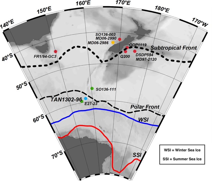
466                                                    J. Jones et al.: Sea ice changes in the SW Pacific over 140 000 years

water mass formation and deep-sea stratification, leading to      (MAT) to fossil diatom assemblages from sediment core
reduced diapycnal mixing and reduced CO2 exchange be-             TAN1302-96 (59.09◦ S, 157.05◦ E, water depth 3099 m). We
tween the surface and deep ocean (Toggweiler, 1999; Bouttes       place this record within the context of sea ice and SSST
et al., 2010; Ferrari et al., 2014). Numerical modelling stud-    changes from the region using previously published records
ies have shown that sea-ice-induced capping, stratification,      from SO136-111 (56.66◦ S, 160.23◦ E, water depth 3912 m),
and reduced vertical mixing may be able to account for a          which has recalculated WSIC and SSST estimates presented
significant portion of the total CO2 variability on glacial–      in this study, and nearby marine core E27-23 (59.61◦ S,
interglacial timescales (between 40–80 ppm) (Stephens and         155.23◦ E, water depth 3182 m) (Ferry et al., 2015). Using
Keeling, 2000; Galbraith and de Lavergne, 2018; Marzoc-           these records, we compare the timing of sea ice expansion
chi and Jansen, 2019; Stein et al., 2020). However, debate        to early glacial–interglacial CO2 variability to test the hy-
continues surrounding the timing and magnitude of sea ice         pothesis that the initial CO2 drawdown (∼ 115 to 100 ka)
impacts on glacial-scale carbon sequestration (e.g., Morales      resulted from reduced air–sea gas exchange in response to
Maquede and Rahmstorf, 2002; Archer et al., 2003; Sun and         sea ice capping and surface water stratification (Kohfeld and
Matsumoto, 2010; Kohfeld and Chase, 2017).                        Chase, 2017). We then consider alternative oceanic drivers of
   Past Antarctic sea ice coverage has been estimated primar-     early atmospheric CO2 variability and place our SSST esti-
ily through diatom-based reconstructions, with most work          mates within the context of other studies to examine how re-
focusing on the Last Glacial Maximum (LGM), specifically          gional cooling and a weakening in meridional SST gradients
the EPILOG time slice as outlined in Mix et al. (2001), cor-      might affect air–sea disequilibrium and early CO2 drawdown
responding to 23 to 19 thousand years before present (ka,         (Khatiwala et al., 2019). Finally, we compare our WSIC es-
calibrated backwards from 1950). During the LGM, these re-        timates with regional reconstructions of Antarctic Interme-
constructions suggest that winter sea ice expanded by 7–10◦       diate Water (AAIW) production and subduction variability
latitude (depending on the sector of the Southern Ocean),         using previously published carbon isotope analyses on ben-
which corresponds to substantial expansion of total winter        thic foraminifera from intermediate to deep-water depths in
sea ice coverage compared to modern observations (Ger-            the southwest Pacific sector of the Southern Ocean, to test
sonde et al., 2005; Benz et al., 2016; Lhardy et al., 2021).      the hypothesis that sea ice expansion is dynamically linked
Currently, only a handful of studies provide quantitative sea     to AAIW production and variability (Ronge et al., 2015).
ice coverage estimates back to the penultimate glaciation,
Marine Isotope Stage (MIS) 6 (∼ 194 to 135 ka) (Gersonde
                                                                  2     Methods
and Zielinksi, 2000; Crosta et al., 2004; Schneider-Mor et
al., 2012; Esper and Gersonde 2014a; Ghadi et al., 2020).         2.1    Study site and age determination
These studies primarily cover the Atlantic sector, with only
one published sea ice record from each of the Indian (SK200-      We reconstruct diatom-based WSIC and SSST using ma-
33 from Ghadi et al., 2020), eastern Pacific (PS58/271-1 from     rine sediment core TAN1302-96 (59.09◦ S, 157.05◦ E, wa-
Esper and Gersonde, 2014a), and southwestern Pacific sec-         ter depth 3099 m) (Fig. 1). The 364 cm core was collected
tors (SO136-111 from Crosta et al., 2004). These glacial–         in March 2013 using a gravity corer during the return of the
interglacial sea ice records show heterogeneity between sec-      RV Tangaroa from the Mertz Polynya in eastern Antarctica
tors in both timing and coverage. While the Antarctic Zone        (Williams, 2013). The core is situated in the western Pacific
(AZ) in the Atlantic sector experienced early sea ice advance     sector of the Southern Ocean, on the southwestern side of
corresponding to MIS 5d cooling (i.e., 115 to 105 ka) (Ger-       the Macquarie Ridge, approximately 3–4◦ south of the aver-
sonde and Zielinksi, 2000; Bianchi and Gersonde, 2002; Es-        age position of the Polar Front (PF) at 157◦ E (Sokolov and
per and Gersonde, 2014a), the Indian and Pacific sector cores     Rintoul, 2009).
in the AZ show only minor sea ice advances during this time          The age model for TAN1302-96 (Figs. 2 and 3) was
(Crosta et al., 2004; Ghadi et al., 2020). The lack of spa-       based on a combination of radiocarbon dating of mixed
tial and temporal resolution has resulted in significant uncer-   foraminiferal assemblages and stable oxygen isotope stratig-
tainty in our ability to evaluate the timing and magnitude of     raphy on Neogloboquadrina pachyderma (180–250 µm).
sea ice change during a full glacial cycle across the Southern    Seven accelerator mass spectrometry (AMS) 14 C samples
Ocean, and to link sea ice to glacial–interglacial CO2 vari-      were collected (Table A1 in Appendix A) and consisted of
ability.                                                          mixed assemblages of planktonic foraminifera (N. pachy-
   This paper provides new winter sea ice concentration           derma and Globigerina bulloides, > 250 µm). Three of the
(WSIC) and summer sea surface temperature (SSST) esti-            seven radiocarbon samples (NZA 57105, 57109, and 61429)
mates for the southwestern Pacific sector of the Southern         were previously published in Prebble et al. (2017), and four
Ocean over the last 140 ka. WSIC, which is a grid-scale ob-       additional samples (OZX 517-520) were added to improve
servation of the mean state fraction of ocean area that is        the dating reliability (Table A1 in Appendix A). OZX 519
covered by sea ice over the sample period, and SSST esti-         and OZX 520 produced dates that were not distinguishable
mates are produced by applying the modern analog technique        from the background (> 57.5 ka) and were subsequently ex-

Clim. Past, 18, 465–483, 2022                                                        https://doi.org/10.5194/cp-18-465-2022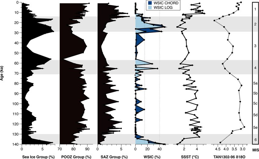
J. Jones et al.: Sea ice changes in the SW Pacific over 140 000 years                                                             467

                                                                        compared to glacial periods, averaging ∼ 2.5 cm ka−1 . It is
                                                                        worth noting that there can be significant MRA variability
                                                                        over time due to changes in ocean ventilation, sea ice cov-
                                                                        erage, and wind strength, specifically in the polar high lati-
                                                                        tudes (Heaton et al., 2020), and as a result, caution should be
                                                                        taken when interpreting the precision of radiocarbon dates.
                                                                        For more information on age model construction and selec-
                                                                        tion, refer to the Supplement.

                                                                        2.2   Diatom analysis
                                                                        TAN1302-96 was sampled every 3–4 cm throughout the core
                                                                        except between 130–180 cm, where samples were collected
                                                                        every 10 cm due to limited availability of sample materi-
                                                                        als (Table A3 in Appendix A). Diatom slide preparation
                                                                        followed two procedures. The first approach approximated
                                                                        the methods outlined in Renberg (1990), while the sec-
                                                                        ond followed the protocol outlined in Warnock and Scherer
                                                                        (2015). To ensure there were no biases between preparation
Figure 1. Map of the southwestern Pacific sector of the Southern
Ocean including the study site, TAN1302-96 (blue circle), and ad-       techniques, results from each technique were first visually
ditional published cores providing sea ice extent data, SO136-111       compared followed by a comparison of sample means (see
and E27-23 (green circles); SST reconstructions (red circles); and      Fig. B1 in Appendix B). No biases in the data were observed
δ 13 C of benthic foraminifera (yellow circles). Note that some cores   between methods.
may not appear present in the figure because of their proximity to         The first procedure was conducted at Victoria University
other cores. Data for all cores are provided in Table 2. Dashed lines   of Wellington and Simon Fraser University on samples ev-
show the average location of the subtropical and polar fronts (Smith    ery 10 cm throughout the core. Sediment samples contained
et al., 2013; Bostock et al., 2015), and red and blue lines show mean   high concentrations of diatoms with little carbonaceous or
positions of modern summer sea ice (SSI) and winter sea ice (WSI)       terrigenous materials, so no dissolving aids were used. In-
extents, respectively (Reynolds et al., 2002, 2007).
                                                                        stead, approximately 50 mg of sediment was weighed, placed
                                                                        into a 50 mL centrifuge tube, and topped up with 40 mL of
                                                                        deionized water. Samples were then manually shaken to dis-
cluded from the age model. The TAN1302-96 oxygen iso-                   aggregate sediment, followed by a 10 s mechanical stir using
topes were run at the National Institute of Water and Atmo-             a vortex machine. Samples were then left to settle for 25 s. A
spheric Research (NIWA) using the Kiel IV individual acid-              total of 0.25 mL of the solution was then pipetted onto a mi-
on-sample device and analysed using Finnigan MAT 252                    croscope slide from a consistent depth, where it was left to
mass spectrometer. The precision is ±0.07 % for δ 18 O and              dry overnight. Once the sample had dried, coverslips were
±0.05 % for δ 13 C.                                                     permanently mounted to the slide using Permount, a high
   The age model was constructed using the “Undatable”                  refractive index mountant. Slides were redone if they con-
MATLAB software (Lougheed and Obrochta, 2018) by boot-                  tained too many diatoms and identification was not possible,
strapping at 10 % and using an xfactor of 0.1 (Lougheed and             or if they contained too few diatoms (generally < 40 speci-
Obrochta, 2019), which scales Gaussian distributions of sed-            mens per transect). Sediment sample weight was adjusted to
iment accumulation uncertainty (Table A2 in Appendix A).                achieve the desired dilution.
Below 100 cm, nine tie points were selected at positions                   The second procedure was conducted at Colgate Univer-
of maximum change in δ 18 O and were correlated to the                  sity on samples every 3–4 cm throughout the core. Oven-
LR04 benthic stack (Lisiecki and Raymo, 2005) (Fig. 2; Ta-              dried samples were placed into a 20 mL vial with 1–2 mL of
ble A2 in Appendix A). Uncertainty associated with strati-              10 % H2 O2 and left to react for up to several days, followed
graphic correlation to the LR04 stack has been estimated to             by a brief (2–3 s) ultrasonic bath to disaggregate samples.
be ±4 ka (Lisiecki and Raymo, 2005). We used a conserva-                The diatom solution was then added into a settling cham-
tive marine reservoir age (MRA) for radiocarbon calibration             ber, where microscope coverslips were placed on stages to
of 1000±100 years, in line with regional estimates in Paterne           collect settling diatoms. The chamber was gradually emp-
et al. (2019) and modelled estimates by Butzin et al. (2017,            tied through an attached spigot, and samples were evapo-
2020). The age model shows that TAN1302-96 extends to at                rated overnight. Cover slips were permanently mounted onto
least 140 ka, capturing a full glacial–interglacial cycle. Lin-         the slides with Norland Optical Adhesive 61, a mounting
ear sedimentation rates in TAN1302-96 were observed to be               medium with a high refractive index.
higher during interglacial periods, averaging ∼ 3.5 cm ka−1 ,

https://doi.org/10.5194/cp-18-465-2022                                                               Clim. Past, 18, 465–483, 2022
468 J. Jones et al.: Sea ice changes in the SW Pacific over 140 000 years
Figure 2. Age model of TAN1302-96. Red circles indicate the depth of AMS 14 C samples, and yellow circles indicate tie points between
the TAN1302-96 oxygen isotope stratigraphy and the LR04 benthic stack (Lisiecki and Raymo, 2005). Two radiocarbon dates, OZX 519 and
520 (at 130 and 170 cm, respectively), were not included in the age model as they produced dates that were NDFB (not distinguishable from
the background).
Diatom identification was conducted at Simon Fraser Uni-
versity using a Leica Leitz DMBRE light microscope us-
ing standard microscopy techniques. Following transverses, a
minimum of 300 individual diatoms were identified at 1000×
magnification from each sample throughout the core. Indi-
viduals were counted towards the total only if they repre-
sented at least one-half of the specimen so that fragmented
diatoms were not counted twice. Identification was con-
ducted to the highest taxonomic level possible, either to the
species or species-group level. Taxonomic identification was
conducted using numerous identification materials, including
(but not limited to) Fenner et al. (1976), Fryxell and Hasle
(1976, 1980), Johansen and Fryxell (1985), Hasle and Syver-
sten (1997), Cefarelli et al. (2010), and Wilks and Armand
(2017). The relative abundances were calculated by dividing
the number of identified specimens of a particular species
by the total number of identified diatoms from the sample.
Based on previously established taxonomic groups (Crosta et
al., 2004), diatoms were grouped into one of three categories
based on temperature preference and sea ice tolerance. The
following main taxonomic groups were used (Table 1):
1. Sea ice group. This represents diatoms that thrive in or
near the sea ice margin in SSTs generally ranging from
Figure 3. Age model of TAN1302-96. Tie points are depicted as −1 to 1 ◦ C.
yellow dots, and grey shading represents associated uncertainty be-
tween tie points. The age model used a marine reservoir calibration
of 1000 ± 100 years. 2. Permanently Open Ocean Zone (POOZ). This repre-
sents diatoms that thrive in open ocean conditions, with
SSTs generally ranging from ∼ 2 to 10 ◦ C.
Clim. Past, 18, 465–483, 2022 https://doi.org/10.5194/cp-18-465-2022J. Jones et al.: Sea ice changes in the SW Pacific over 140 000 years 469
3. Sub-Antarctic Zone (SAZ). This represents diatoms that 3 Results
thrive in warmer sub-Antarctic waters, with SSTs gen-
erally ranging from 11 to 14 ◦ C. 3.1 TAN1302-96 diatom assemblage results
In this core, 51 different species or species groups were iden-
tified, of which 33 were used in the transfer function. These
2.3 Modern analog technique
33 species represent > 82 % of the total diatom assemblages
Past WSIC and SSST (January to March) were estimated for (mean of 92 %). Permanently Open Ocean Zone (POOZ) di-
TAN1302-96 and recalculated for SO136-111 by applying atoms made up the largest proportion of diatoms identified,
the modern analog technique (MAT) to the fossil diatom as- representing between 72 %–91 % of the assemblage (Fig. 4),
semblages, as outlined in Crosta et al. (1998, 2020). Summer with higher values observed during warmer interstadial peri-
(January to March) SST was estimated because it is consid- ods of MIS 1, 3, and 5. Sea ice diatoms made up the second
ered to be a better explanatory variable than spring or an- most abundant group, representing between 0.5 %–7.5 % of
nual SST (Esper et al., 2010; Esper and Gersonde, 2014b). the assemblage, with higher values observed during cooler
The MAT reference database used for this analysis is com- stadial periods (MIS 2, 4, and 6). The Sub-Antarctic Zone
prised of 249 modern core top samples (analogs) located group had relatively low abundances, with higher values oc-
primarily in the Atlantic and Indian sectors from ∼ 40◦ S curring during warmer interstadial periods (MIS 5 and the
to the Antarctic coast. The age of the core tops included Holocene) and briefly during MIS 4 at ∼ 65 ka.
in the reference database have been assessed through ra-
diocarbon and/or isotope stratigraphy when possible. Core 3.2 TAN1302-96 SSST and WSIC estimates
tops were visually evaluated for selective diatom dissolu-
tion, so it is believed that sub-modern assemblages contain There were no non-analog conditions observed in TAN1302-
well-preserved and unbiased specimens. Modern SSST and 96 samples, and all estimates were calculated on five analogs.
WSIC were interpolated from the reference core locations Estimates of SSST and WSIC from both LOG and CHORD
using a 1◦ × 1◦ grid from the World Ocean Atlas (Locarnini MAT outputs produced similar results (Fig. 4). During Ter-
et al., 2013) through the Ocean Data View (Schlitzer, 2005). mination II, SSST began to rise from ∼ 1 ◦ C at 140 ka
The MAT was applied using the “bioindic” package (Guiot (MIS 6) to ∼ 4.5 ◦ C at 132 ka (MIS 5e–6 boundary). This
and de Vernal, 2011) through the R platform. Fossil diatom warming corresponded with a decrease in WSIC from 48 %
assemblages were compared to the modern analogs using to approximately 0 % over the same time periods (Fig. 4). Re-
33 species or species groups to identify the five most sim- constructed SSSTs were variable throughout MIS 5e, reach-
ilar modern analogs using both the LOG and CHORD dis- ing a maximum value of ∼ 4.5 ◦ C at 118 ka, after which they
tance. The dissimilarity threshold, above which the fossil as- declined throughout MIS 5. During this period of SSST de-
semblages are considered to be too dissimilar to the mod- cline, winter sea ice was largely absent, punctuated by brief
ern dataset, is fixed at the first quartile of random distances periods during which sea ice was present but unconsolidated
(Crosta et al., 2020). The reconstructed SSST and WSIC are (WSIC =∼ 15 % and 17 % at 105 and 85 ka, respectively).
the distance-weighted mean of the climate values associated During MIS 4 (71 to 57 ka), SSST cooled to between roughly
with the selected modern analog (Guiot et al., 1993; Ghadi 1 and 3 ◦ C, and sea ice expanded to 36 %, such that it was
et al., 2020). Both MAT approaches produce an R 2 value of present but unconsolidated for intervals of a few thousand
0.96 and a root mean square error of prediction (RMSEP) of years. SSST increased slightly from 1.5 ◦ C at 61 ka (during
∼ 1 ◦ C for SSST and an R 2 of 0.93 and a RMSEP of 10 % for MIS 4) to ∼ 2.5 ◦ C at 50 ka (during MIS 3), followed by a
WSIC (Ghadi et al., 2020). As outlined in Ferry et al. (2015), general cooling trend into MIS 2. Sea ice appears to have
we consider < 15 % WSIC to represent an absence of winter been largely absent during MIS 3 (57 to 29 ka), although
sea ice, 15 %–40 % WSIC as present but unconsolidated, and sampling resolution is low, but increased rapidly to 48 %
> 40 % to represent consolidated winter sea ice. cover during MIS 2 where winter sea ice was consolidated
over the core site. During MIS 2, SSST cooled to a minimum
of < 1 ◦ C at 24.5 ka. After 18 ka, the site rapidly transitioned
2.4 Additional core data
from cool, ice-covered conditions to warmer, ice-free win-
We use additional published marine cores from the south- ter conditions during the early deglaciation. This warming
western Pacific throughout this analysis (Table 2), for was interrupted by a brief cooling around 13.5 ka, follow-
WSIC comparisons (E27-23), %AAIW calculations (MD06- ing which SSSTs quickly reached their maximum values of
2990/SO136-003, MD06-2986, and MD97-2120), and re- ∼ 5 ◦ C at 11.5 ka and remained relatively high throughout the
gional SST gradient comparisons (SO136-003, FR1/94-GC3, rest of the Holocene. Winter sea ice was not present during
ODP 1119-181, DSDP 594, and Q200). the Holocene.
https://doi.org/10.5194/cp-18-465-2022 Clim. Past, 18, 465–483, 2022470 J. Jones et al.: Sea ice changes in the SW Pacific over 140 000 years
Table 1. Species comprising each of the diatom taxonomic groups (updated from Crosta et al., 2004).
Sea ice group POOZ group SAZ group
Actinocyclus actinochilus Fragilariopsis kerguelensis Azpeitia tabularis
Fragilariopsis curta Fragilariopsis rhombica Hemidiscus cuneiformis
Fragilariopsis cylindrus Fragilariopsis separanda Thalassionema nitzschioides var. lanceolata
Fragilariopsis obliquecostata Rhizosolenia polydactyla var. polydactyla Thalassiosira eccentrica
Fragilariopsis ritscheri Thalassionema nitzschioides (form 1) Thalassiosira oestrupii group
Fragilariopsis sublinearis Thalassiosira gracilis group
Thalassiosira lentiginosa
Thalassiosira oliverana
Thalassiothrix sp.
Trichotoxon reinboldii
Table 2. Additional data on published marine cores used throughout this analysis.
Core name Latitude Longitude Depth Age model reference Data assessed Data source
TAN1302-96 59.09◦ S 157.05◦ E 3099 m This study WSIC; SST This study
SO136-111 56.66◦ S 160.23◦ E 3912 m Crosta et al. (2004) WSIC; SST Crosta et al. (2004),
recalculated in this study
E27-23 57.65◦ S 155.23◦ E 3182 m Ferry et al. (2015) WSIC Ferry et al. (2015)
MD06-2990 42.01◦ S 169.92◦ E 943 m Ronge et al. (2015) δ 13 C Ronge et al. (2015)
MD06-2986 43.45◦ S 167.9◦ E 1477 m Ronge et al. (2015) δ 13 C Ronge et al. (2015)
MD97-2120 45.54◦ S 174.94◦ E 1210 m Pahnke and Zahn (2005) δ 13 C Pahnke and Zahn (2005)
SO136-003 42.3◦ S 169.88◦ E 958 m Pelejero et al. (2006), δ 13 C; SST Pelejero et al. (2006),
Barrows et al. (2007) Ronge et al. (2015)
FR1/94-GC3 44.25◦ S 149.98◦ E 2667 m Pelejero et al. (2006) SST Pelejero et al. (2006)
ODP 1119-181 44.75◦ S 172.39◦ E 396 m Wilson et al. (2005) SST Wilson et al. (2005),
Hayward et al. (2008)
DSDP 594 45.54◦ S 174.94◦ E 1204 m Nelson et al. (1985), SST Schaefer et al. (2005)
Kowalski and Meyers (1997)
Q200 45.99◦ S 172.02◦ E 1370 m Waver et al. (1998) SST Weaver et al. (1998)
3.3 SO136-111 SSST and WSIC recalculation during MIS 5, with a brief period where sea ice was present
but unconsolidated (WSIC = 17 % at 84 ka). Beginning at
In core SO136-111, the 33 species included in the transfer ∼ 76 ka, WSIC began to increase and continued throughout
function represent values > 79 % of the total diatom assem- early MIS 4 to a maximum 36 % at 69 ka. WSIC remained
blages (mean of 91 %). There were no non-analog conditions present but unconsolidated throughout most of MIS 3 and 2
observed in SO136-111 samples, and all estimates were cal- with brief periods of absence (WSIC ≤ 15 %) lasting a few
culated on five analogs. Recalculated estimates of SSST and thousand years. SSST and WSIC reached their coolest val-
WSIC from both LOG and CHORD MAT outputs produced ues and highest concentration at 24.5 ka before SSST in-
similar results for SO136-111 (Fig. 5a, d). During Termi- creased to ∼ 5 ◦ C and stabilized throughout the Holocene,
nation II, SSST rose from ∼ 2 ◦ C at 137 ka (MIS 6) to a while WSIC declined to virtually 0 % throughout the same
maximum value of 6 ◦ C at 125 ka (MIS5e), corresponding period.
to a rapid decline in WSIC from 37 % to ∼ 0 % during the
same period. SSST remained relatively high (between 4 and
5 ◦ C) from 125 ka until 115 ka where they declined to ∼ 2 ◦ C.
SSST remained variable from 110 ka until ∼ 40 ka, fluctuat-
ing between ∼ 2 and 4 ◦ C. Winter sea ice was largely absent
Clim. Past, 18, 465–483, 2022 https://doi.org/10.5194/cp-18-465-2022J. Jones et al.: Sea ice changes in the SW Pacific over 140 000 years 471
Figure 4. Diatom assemblages results from TAN1302-96 separated into percentage contribution from each taxonomic group (sea ice group,
POOZ, and SAZ; see Table 1) over a full glacial–interglacial cycle. Using the modern analog technique (MAT), winter sea ice concentration
(WSIC) and summer sea surface temperature (SSST) were estimated and compared against the δ 18 O signature of TAN1302-96.
4 Discussion the mid-Holocene (∼ 6 ka), while TAN1302-96 experienced
values well below the RMSEP of 10 %.
4.1 Regional SSST and WSIC estimates Possible explanations for the observed differences in
WSIC estimates include (1) differences in statistical appli-
cations, (2) lateral sediment redistribution, (3) differences
The new WSIC and SSST estimates from TAN1302-96
in laboratory protocols, (4) differences in diatom identifica-
and recalculated WSIC estimates from SO136-111 show
tion/counting methodology, and (5) selective diatom dissolu-
a coherent regional pattern (Fig. 5). TAN1302-96 shows
tion. Of these explanations, we believe that (1) and (2) are
slightly higher concentrations during MIS 2 (maximum
the most likely candidates and are discussed below (for fur-
WSIC = 48 % at 24.5 ka) and 4 (maximum WSIC = 37 % at
ther discussion on 3, 4, and 5, see Appendix C).
65 ka) compared with SO136-111 (maximum WSIC = 35 %
The first possible explanation is the use of different sta-
at 24.5 ka and 36 % at 68 ka, respectively), which can be ex-
tistical applications. Ferry et al. (2015) used a generalized
plained by a more poleward position of TAN1302-96 rela-
additive model (GAM) to estimate WSIC for both E27-23
tive to SO136-111. The estimates between cores differ dur-
and SO136-111, while we have used the MAT for TAN1302-
ing MIS 3, with seemingly lower WSIC in TAN1302-96 than
96 and SO136-111. A simple comparison of WSIC estimates
in SO136-111, which might result from the low sampling
between the results in Ferry et al. (2015) and our recalculated
resolution in TAN1302-96 during this period. Overall, these
WSIC estimates for SO136-111 can provide insights into the
cores show a highly similar and coherent history of sea ice
magnitude of estimation differences. Generally speaking, the
over the last 140 ka.
GAM estimation produced higher WSIC estimates than the
When compared with E27-23 (Fig. 5b), which is located
MAT (e.g., ∼ 50 % WSIC at 23 ka while the MAT produced
only ∼ 120 km to the southwest of TAN1302-96 (Fig. 1),
∼ 37 % for the same time period); however, we believe it
the TAN1302-96 core shows lower estimates of WSIC, es-
is unlikely that statistical approaches alone could explain a
pecially during MIS 3. During early and mid-MIS 2, both
larger difference (i.e., 50 %) between E27-23 and TAN1302-
cores show similar WSIC estimates, while later in MIS 2
96.
(∼ 17 ka), E27-23 reports a maximum WSIC of 72 % com-
The second possible explanation involves lateral sediment
pared to only 22 % at TAN1302-96. A discrepancy between
redistribution and focusing by the ACC. We estimated sedi-
estimates is also observed during the Holocene, with E27-
ment focusing for E27-23 using 230 Th data from Bradtmiller
23 reporting sea ice estimates of up to nearly 50 % during
https://doi.org/10.5194/cp-18-465-2022 Clim. Past, 18, 465–483, 2022472 J. Jones et al.: Sea ice changes in the SW Pacific over 140 000 years
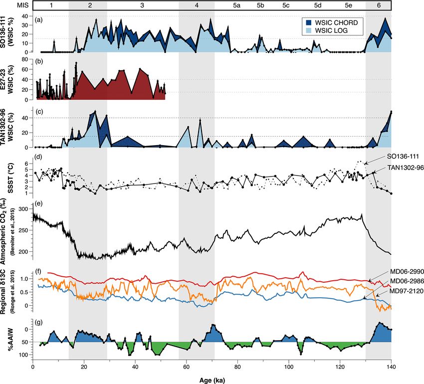
Figure 5. (a) WSIC estimates using MAT from SO136-111 (recalculated in this study; see Appendix D); (b) WSIC estimates using GAM
from E27-23 (Ferry et al., 2015); (c) WSIC estimates using MAT from TAN1302-96 (this study); (d) SSST estimates using MAT from
TAN1302-96 (solid black line) and recalculated SSST for SO136-111 (black dotted line); (e) Antarctic atmospheric CO2 concentrations over
140 ka (Bereiter et al., 2015); (f) δ 13 C data from nearby cores MD06-2990/SO136-003, MD97-2120, and MD06-2986 (Ronge et al., 2015);
(g) %Antarctic Intermediate Water (%AAIW) as calculated in Ronge et al. (2015), which tracks when core MD97-2120 was bathed primarily
by AAIW (green) or Upper Circumpolar Deep Water (UCDW) (blue).
et al. (2009) together with dry bulk density estimated using the scope of this study; however, future work could help ad-
calcium carbonate content (Froelich, 1991). Both sedimenta- dress this uncertainty.
tion rates and focusing factors (FF) for the E27-23 are rel- Although we are unable to identify the specific cause of
atively high (maximum ∼ = 35 cm ka−1 and 26, respectively) the differences, we suggest considering the results from all
during the LGM and Holocene, which could influence the cores when drawing conclusions of regional sea ice history.
reliability of WSIC and SSST estimation (see Fig. C1 in Ap-
pendix C). Several peaks in focusing occurring around 16,
12, and 3 ka appear to closely correspond to periods of peak 4.2 The role of sea ice on early CO2 drawdown
WSIC (∼ 67 %, ∼ 54 %, and ∼ 35 %, respectively), suggest- Kohfeld and Chase (2017) hypothesized that the initial draw-
ing a possible link. Lateral redistribution could artificially down of atmospheric CO2 (∼ 35 ppm) during the glacial in-
increase or decrease relative abundances of some diatom ception of MIS 5d (∼ 115 to 100 ka) was primarily driven
groups, which could lead to over- or under-estimations of sea by sea ice capping and a corresponding stratification of sur-
ice coverage. Thorium analysis for TAN1302-96 is beyond face waters, which reduced the CO2 outgassing of upwelled
carbon-rich waters. This hypothesis is supported by sev-
Clim. Past, 18, 465–483, 2022 https://doi.org/10.5194/cp-18-465-2022J. Jones et al.: Sea ice changes in the SW Pacific over 140 000 years 473 eral lines of evidence, including (1) sea salt sodium (ssNA) can be linked solely to the capping and stratification effects archived in Antarctic ice cores, suggesting sea ice expansion of sea ice expansion. near the Antarctic continent (Wolff et al., 2010); (2) δ 15 N proxy data from the central Pacific sector of the South- 4.3 Other potential contributors to early glacial CO2 ern Ocean, suggesting increased stratification south of the variability modern-day Antarctic Polar Front (Studer et al., 2015); and (3) diatom assemblages in the Permanently Open Ocean The changes observed in WSIC and SSST from TAN1302- Zone (POOZ) of the Atlantic sector, suggesting a slight 96 suggest that sea ice expansion was likely not extensive cooling and northward expansion of sea ice during MIS 5d enough early in the glacial cycle for a sea ice capping ef- (Bianchi and Gersonde, 2002). Our data address this hypoth- fect to be solely responsible for early atmospheric CO2 draw- esis by providing insights into early sea ice expansion into down. This leaves open the question of what may have con- the polar frontal zone of the western Pacific sector. tributed to early drawdown of atmospheric CO2 . In terms of Our data show that, in contrast to the Atlantic sector the ocean’s role, we highlight three contenders: (1) a poten- (Bianchi and Gersonde, 2002), there does not appear to be tially non-linear response between sea ice coverage and CO2 any evidence of sea ice expansion in the southwestern Pa- sequestration potential, (2) links between sea ice expansion cific during MIS 5d at either the TAN1302-96 or SO136-111 and early changes in global ocean overturning, and (3) the core sites (Fig. 5). Unfortunately, the lack of spatially ex- impact of cooling on air–sea disequilibrium in the Southern tensive quantitative records extending back to Termination II Ocean. limits our ability to estimate the timing and magnitude of sea The first possible explanation considers that not all sea ice ice changes for regions poleward of 59◦ S in the southwest- has the same capacity to facilitate or inhibit air–sea gas ex- ern Pacific. We anticipate, however, that an advance in the change. We previously suggested that because sea ice was sea ice edge, consistent with those outlined in Bianchi and not at its maximum extent during MIS 5d, the contribution Gersonde (2002), likely would have reduced local SST as of sea ice on CO2 sequestration would likely not be at its the sea ice edge advanced closer to the core site. Indeed, the maximum extent either. However, this assumes a linear re- TAN1302-96 SSST record does show a decrease to ∼ 2 ◦ C lationship between sea ice coverage and CO2 sequestration (observed at 108 ka), which quickly rebounded to ∼ 4 ◦ C by potential. We know that different sea ice properties, such as ∼ 102 ka (Fig. 5). However, this SSST drop occurred roughly thickness and temperature, determine overall porosity, with 7 ka after the initial CO2 reduction, suggesting that the CO2 thicker and colder sea ice being less porous and more ef- drawdown event and local SSST reduction may not be linked. fective at reducing air–sea gas exchange compared to thin- Thus, while we cannot rule out the possibility of modest sea ner and warmer sea ice (Delille et al., 2014). It is therefore ice advances or consolidation of pre-existing sea ice (partic- possible that if modest sea ice advances took place closer to ularly to the south of the core sites), the quantitative WSI and the Antarctic continent (and were therefore not captured by SSST reconstructions suggest that sea ice cover over our core TAN1302-96), they may have been more effective at reduc- site was limited during glacial inception. ing CO2 outgassing either by experiencing some type of reor- Given that sea ice was not at its maximum extent during ganization or consolidation, or through a change in properties the early glacial, it stands to reason that any reductions to such as temperature or thickness. It is also possible that sea air–sea gas exchange in response to the hypothetically ex- ice coverage over some regions leads to more effective cap- panded sea ice would not have been at its maximum im- ping, while in other regions sea ice growth contributes only pact either. Previous modelling work has suggested that the to marginal reductions in air–sea gas exchange. This, theoret- maximum impact of sea ice expansion on glacial–interglacial ically, could point to a non-linear response between sea ice atmospheric CO2 reductions ranged from 5 to 14 ppm (Ko- expansion and CO2 sequestration potential, and thus mod- hfeld and Ridgwell, 2009). More recent modelling studies est sea ice growth around the Antarctic continent could have are consistent with this range, suggesting a 10 ppm reduc- contributed in part to the ∼ 35 ppm initial CO2 drawdown tion (Stein et al., 2020), while some studies even suggest event. While this is theoretical and cannot be adequately ad- a possible increase in atmospheric CO2 concentrations due dressed in this analysis, it is worthy of deeper consideration. to sea ice expansion (Khatiwala et al., 2019). Furthermore, The second possible explanation involves changes in the Stein et al. (2020) suggest that the effects of sea ice cap- global overturning circulation. Kohfeld and Chase (2017) ping would have taken place after changes in deep ocean previously examined the timing of changes in δ 13 C of benthic stratification had occurred and would have contributed to foraminifera solely from the Atlantic basin and observed that CO2 drawdown later during the mid-glacial period. These the largest changes in the Atlantic Meridional Overturning model results, when combined with our data, suggest that Circulation (AMOC) coincided with the mid-glacial reduc- even if modest sea ice advances did take place during the tions in atmospheric CO2 changes mentioned above. Subse- early glacial (i.e., MIS 5d), their impacts on CO2 variability quent work of O’Neill et al. (2021) examined whole-ocean likely would have been modest, ultimately casting doubt on changes in δ 13 C of benthic foraminifera and noted that the the hypothesis that early glacial CO2 reductions of 35 ppm separation between δ 13 C values of abyssal and deep ocean https://doi.org/10.5194/cp-18-465-2022 Clim. Past, 18, 465–483, 2022
474                                                    J. Jones et al.: Sea ice changes in the SW Pacific over 140 000 years

waters – and therefore the isolation of the abyssal ocean –       cle. The annual growth and decay of Antarctic sea ice plays
was actually initiated between MIS 5d and MIS 5a (114 to          a critical role in regional water mass formation. Brine rejec-
71 ka). Evidence for early changes in abyssal circulation and     tion results in net buoyancy loss in regions of sea ice forma-
reductions in deep-ocean overturning have also been detected      tion, while subsequent melt results in freshwater inputs and
in Indian Ocean δ 13 C records (Govin et al., 2009). More         net buoyancy gains near the ice margin (Shin et al., 2003;
recently, Indian Ocean εNd records (Williams et al., 2021)        Pellichero et al., 2018). This increased freshwater input and
have suggested that the abyssal ocean may have responded          buoyancy gain near the ice margin can hinder AAIW sub-
to sea ice changes around the Antarctic continent early in the    duction, with direct and indirect impacts on both the upper
glacial cycle, with colder and more saline AABW forming           and lower branches of the meridional overturning circulation
as sea ice expanded near the continent. If indications of an      (Pellichero et al., 2018).
early-glacial response in the global ocean circulation in the        Previous research has used δ 13 C in benthic foraminifera to
Indo-Pacific are correct, these data may also point to an el-     track changes in the depth of the interface between AAIW
evated importance of sea ice near the Antarctic continent in      and Upper Circumpolar Deep Water (UCDW) (Pahnke and
triggering early, deep-ocean overturning changes.                 Zahn, 2005; Ronge et al., 2015). Low δ 13 C values are linked
   The third possible explanation involves changes in sur-        to high nutrient concentrations found at depths below ∼
face ocean temperature gradients in the Southern Ocean, and       1500 m in the UCDW, and higher δ 13 C values are associ-
how they could influence air–sea gas exchange. Several re-        ated with the shallower AAIW waters (Fig. 5). Marine sed-
cent studies have pointed to the importance of changes to         iment core MD97-2120 (45.535◦ S, 174.9403◦ E, core depth
air–sea disequilibrium as a key contributor to CO2 uptake in      1210 m) was retrieved from a water depth near the interface
the Southern Ocean (Eggleston and Galbraith, 2018; Mar-           between the AAIW and UCDW water masses (Pahnke and
zocchi and Jansen, 2019; Khatiwala et al., 2019). Khatiwala       Zahn, 2005). Over the last glacial–interglacial cycle, fluc-
et al. (2019) suggested that modelling studies have tradition-    tuations in the benthic δ 13 C values from MD97-2120 sug-
ally underrepresented (or neglected) the role of air–sea dise-    gest that the core site was intermittently bathed in AAIW
quilibrium in amplifying the impact of cooling on potential       and UCDW, and that the vertical extent of AAIW fluctu-
CO2 sequestration in the middle to high southern latitudes        ated throughout the last glacial–interglacial cycle. Ronge et
during glacial periods. They argue that when the full effects     al. (2015) used the δ 13 C values from MD97-2120 and other
of air–sea disequilibrium are considered, ocean cooling can       core sites to quantify the contributions of AAIW to the waters
result in a 44 ppm decrease due to temperature-based solubil-     overlying MD97-2120 (%AAIW, Appendix D). These results
ity effects alone. They attributed this increased impact of SST   suggest that during warm periods, MD97- 2120 exhibited
to a reduction in sea-surface temperature gradients explicitly    more positive δ 13 C values, corresponding to higher %AAIW,
in polar mid-latitude regions (roughly between 40 and 60◦         while cooler periods exhibited more negative values, corre-
north and south). If we compare the SST gradients in the          sponding to lower %AAIW (Fig. 5). This suggests that dur-
southwest Pacific sector over the last glacial–interglacial cy-   ing cooler periods, the AAIW-UCDW interface shoaled, re-
cle (Fig. 6), we see an early cooling response between MIS        ducing the total volume of AAIW and indirectly causing an
5e–d corresponding to roughly half of the full glacial cool-      expansion of UCDW (Ronge et al., 2015).
ing, specifically in the cores located south of the modern STF.      Our comparison between %AAIW and regional WSIC
While they did not quantify them, Bianchi and Gersonde            estimates suggest a strong link between the two (Fig. 5).
(2002) also described a weakening of meridional SST gra-          Specifically, we observe that AAIW shoaled and UCDW ex-
dients between the Subantarctic and Antarctic Zones during        panded (i.e., %AAIW is low) during periods when sea ice ex-
MIS 5d in the Atlantic sector. Although this analysis is based    pansion occurred. In contrast, during periods of low WSIC, a
on sparse data, our SSST reconstructions are consistent with      reduced seasonal sea ice cycle, and warmer summer sea sur-
the notion that surface ocean cooling, a weakening of merid-      face temperatures (e.g., MIS 5e), %AAIW is observed to be
ional SST gradients, and changes to the overall air–sea dise-     high. This correlation supports the idea that increased con-
quilibrium could be responsible for at least some portion of      centrations of regional sea ice resulted in a substantial sum-
the early CO2 drawdown. Further SST estimates from the re-        mer freshwater flux into the AAIW source region. This re-
gion, and from the global ocean, are needed to substantiate       gional freshening likely promoted a shallower subduction of
this hypothesis.                                                  AAIW and a corresponding volumetric expansion of UCDW,
                                                                  which can be seen by the isotopic offset of the δ 13 C val-
4.4   Sea ice expansion and ocean circulation
                                                                  ues between the reference cores, and also by the increased
                                                                  carbonate dissolution in MD97-2120 during glacial periods
Although the TAN1302-96 WSIC record suggests that sea             (Fig. 7) (Pahnke et al., 2003; Ronge et al., 2015). These find-
ice was largely absent at the core site until the mid-glacial     ings directly link sea ice proxy records to observed changes
(∼ 65 ka), the observed changes in sea ice could have mod-        in ocean circulation and water mass geometry.
ulated regional fluctuations in Antarctic Intermediate Water         In addition to its influence on regional freshwater forc-
(AAIW) subduction throughout the glacial–interglacial cy-         ing and AAIW reductions, these sea ice changes may also

Clim. Past, 18, 465–483, 2022                                                         https://doi.org/10.5194/cp-18-465-2022
J. Jones et al.: Sea ice changes in the SW Pacific over 140 000 years 475 Figure 6. SST estimates from seven cores located in the southwestern Pacific. SST used were five-point averages (depending on sampling resolution) taken at MIS peaks and median dates in accordance with boundaries outlined in Lisiecki and Raymo (2005). Due to the complex circulation and frontal structures in the region, cores were plotted in ± distance from the average position of the modern STF. Cores used include SO136-003 (SSTs calculated from alkenones, Pelejero et al., 2006), FR1/94-GC3 (alkenones, Pelejero et al., 2006), ODP 181-1119 (PF-MAT, Hayward et al., 2008), DSDP594 (PF-MAT, Schaefer et al., 2005), Q200 (PF-MAT, Weaver et al., 1998), SO136-111 (D-MAT, Crosta et al., 2004), and TAN1302-96 (D-MAT; this study). The blue band represents the modern STF zone, while the red dotted line represents the southern shift in the STF during MIS 5e (Cortese et al., 2013). coincide with larger-scale deep ocean circulation changes. ulations suggest a resulting CO2 sequestration of 20–40 ppm The most dramatic increases in winter sea ice observed into the deep ocean. in TAN1302-96 and SO136-111, along with changes in Taken collectively, the available data show that sea ice %AAIW, are initiated during MIS 4. These shifts also cor- expansion, AAIW-UCDW shoaling, changes in the AMOC, respond to basin-wide changes in benthic δ 13 C values in the and a decrease in atmospheric CO2 all occur concomitantly Atlantic Ocean that suggest a shoaling in the AMOC dur- during MIS 4 (Fig. 5). It appears likely, therefore, that sea ing MIS 4 (Oliver et al., 2010; Kohfeld and Chase, 2017). ice expansion during this time influenced intermediate wa- Changes in deep ocean circulation are also recorded in εNd ter density gradients through increased freshening and con- isotope data in the Indian sector of the Southern Ocean sequent shoaling of AAIW, which may also have increased (Wilson et al., 2015), suggesting extensive reductions in the the efficiency of the carbon pump and increased CO2 uptake AMOC during this period. Recent modelling literature (Mar- by phytoplankton (Sigman et al., 2021). This appears to have zocchi and Jansen, 2019; Stein et al., 2020) suggests that sea occurred while simultaneously influencing deep-ocean den- ice formation directly impacts marine carbon storage by in- sity, and therefore stratification, through brine rejection and creasing density stratification and reducing diapycnal mix- enhanced deep water formation, which ultimately lead to de- ing, especially in simulations where brine rejection is en- creased ventilation (Abernathey et al., 2016). These changes hanced near the Antarctic continental slope and open ocean in ocean stratification, combined with the sea ice “capping” vertical mixing (and subsequent CO2 outgassing) is reduced mechanism, appear to agree with both the recent modelling (Bouttes et al., 2010, 2012; Menviel et al., 2012). These sim- efforts (Stein et al., 2020) and observed proxy data and fit https://doi.org/10.5194/cp-18-465-2022 Clim. Past, 18, 465–483, 2022
476                                                       J. Jones et al.: Sea ice changes in the SW Pacific over 140 000 years

Figure 7. Schematic of changes in southwestern Pacific sector sea ice coverage and water mass geometry between interglacial and glacial
stages. Panel (a) depicts interglacial conditions where sea ice coverage is minimal and freshwater input from summer sea ice melt is low.
This lack of freshwater input allows AAIW to subduct to deeper depths and bath core MD97-2120, capturing the higher δ 13 C signature of
the overlying AAIW waters. The AAIW-UCDW interface (red dashed line) is located beneath MD97-2120. CO2 outgassing is occurring as
a carbon-rich Circumpolar Deep Water upwell near Antarctica. Panel (b) depicts glacial conditions where sea ice expansion has occurred
beyond TAN1302-96, increasing brine rejection, and stabilizing the water column. As a result of the increased sea ice growth, subsequent
summer melt increases the freshwater flux into the AAIW source region and increases AAIW buoyancy. This buoyancy gain shoals the
AAIW-UCDW interface above core MD97-2120, causing the core site to be bathed in low δ 13 C UCDW. The shoaling of AAIW causes an
indirect expansion of CDW, increasing the glacial carbon stocks of the deep ocean, while sea ice reduces CO2 outgassing via the capping
mechanism.

well within the hypothesis that mid-glacial CO2 variability            al., 2019). Another key consideration is the potentially non-
was primarily the result of a more sluggish overturning cir-           linear response between sea ice expansion and CO2 seques-
culation (Kohfeld and Chase, 2017).                                    tration potential (i.e., that not all sea ice is equal in its ca-
                                                                       pacity to sequester carbon). More analyses are required to
                                                                       adequately address this.
5   Summary and conclusion
                                                                          We also observe a strong link between regional sea ice
This study presents new WSIC and SSST estimates from                   concentrations and vertical fluctuations in the AAIW-UCDW
marine core TAN1302-96, located in the southwestern Pa-                interface. Regional sea ice expansion appears to coincide
cific sector of the Southern Ocean. We find that the WSIC              with the shoaling of AAIW, likely due to the freshwater flux
remained low during the early glacial cycle (130 to 70 ka),            from summer sea ice melt increasing buoyancy in the AAIW
expanded during the middle glacial cycle (∼ 65 ka), and                formation region. Furthermore, major sea ice expansion and
reached its maximum just prior to the LGM (∼ 24.5 ka).                 AAIW shoaling occurs during the middle of the glacial cy-
These results largely agree with nearby core SO136-111 but             cle and is coincident with previously recognized shoaling in
display some differences in WSIC magnitude with E27-23.                AMOC and mid-glacial atmospheric CO2 reductions, sug-
This discrepancy may be explained by differences in sta-               gesting a mechanistic link between sea ice and ocean circu-
tistical applications and/or lateral sediment redistribution,          lation.
although more analysis is required to determine the exact                 In conclusion, this paper has focused exclusively on sea
cause(s).                                                              ice as a driver of physical changes, but we recognize that
   The lack of changes in SSST and the absence of winter sea           these changes in sea ice will be accompanied by multiple
ice over the core site during the early glacial suggests that          processes that interact and compete with each other. Marzoc-
the sea ice capping mechanism and corresponding surface                chi and Jansen (2019) note that teasing apart the individual
stratification in this region is an unlikely cause for early CO2       components of CO2 fluctuations is complicated because of
drawdown, and that alternative hypotheses should be consid-            interactions between sea ice capping, air–sea disequilibrium,
ered when evaluating the mechanism(s) responsible for the              AABW formation rates, and the biological pump. We recog-
initial drawdown. More specifically, we consider the impact            nize that these processes may not act independently and, as
of changes in SSST gradients between ∼ 40 to 60◦ S and                 such, have contributed new data to help advance our collec-
support the idea that changes in air–sea disequilibrium asso-          tive understanding of the role of sea ice on influencing atmo-
ciated with reduced sea-surface temperature gradients could            spheric CO2 variability on a glacial–interglacial timescale.
be a potential mechanism that contributed to early glacial re-
ductions in atmospheric CO2 concentrations (Khatiwala et

Clim. Past, 18, 465–483, 2022                                                               https://doi.org/10.5194/cp-18-465-2022
J. Jones et al.: Sea ice changes in the SW Pacific over 140 000 years 477
Appendix A: Age model and sampling depths
Table A1. Radiocarbon dates taken from TAN1302-96. NDFB = not distinguishable from the background.
Lab code Sample material Core name Depth δ 13 C δ 13 C % modern 1σ Modern (+/−) Radiocarbon 1σ Reference
(cm) (per mil) (+/−) carbon error fraction year error
NZA 57105 N. pachyderma TAN1302-96 21 1 0.2 / / 0.5982 0.0018 4127 24 Prebble et
and G. bulloides al. (2017)
NZA 57109 N. pachyderma TAN1302-96 50 0.7 0.2 / / 0.3723 0.0015 7936 32 Prebble et
and G. bulloides al. (2017)
OZX 517 N. pachyderma TAN1302-96 63 1 0.1 30.62 0.15 / / 9505 40 This study
and G. bulloides
NZA 61429 N. pachyderma TAN1302-96 75 0.7 0.2 / / 0.2373 0.0011 11 554 37 Prebble et
and G. bulloides al. (2017)
OZX 518 N. pachyderma TAN1302-96 87 −0.1 0.1 19.62 0.11 / / 13 085 45 This study
and G. bulloides
OZX 519 N. pachyderma TAN1302-96 130 1.7 0.1 0.02 0.04 / / NDFB / This study
and G. bulloides
OZX 520 N. pachyderma TAN1302-96 170 −1.1 0.3 0.03 0.04 / / NDFB / This study
and G. bulloides
Table A2. Tie points used in construction of the TAN1302-96 age model.
TAN1302-96 depth (cm) TAN1302-96 δ 18 O LR04 Age LR04 δ 18 O
110 4.710 18 000 5.02
170 3.930 56 000 4.35
200 3.782 70 000 4.32
220 3.07 82 000 3.8
230 3.23 87 000 4.18
250 3.22 109 000 4.12
270 2.90 123 000 3.1
300 3.660 129 000 3.9
320 4.350 140 000 4.98
https://doi.org/10.5194/cp-18-465-2022 Clim. Past, 18, 465–483, 2022478 J. Jones et al.: Sea ice changes in the SW Pacific over 140 000 years
Table A3. Sample depth and corresponding age. Diatom slides using Method 1 used even-numbered sediment samples (e.g., 10, 20, 30),
while diatom slides using Method 2 used odd-numbered sediment samples (e.g., 53, 87).
Sample depth (cm) Age Sample depth (cm) Age Sample depth (cm) Age Sample depth (cm) Age
10 1001∗ 100 16 011 197 68 608 260 116 007
20 2531∗ 103 16 609 200 69 999 263 118 110
30 4061 107 17 406 203 71 790 267 120 912
40 5591 110 18 000 207 74 196 270 123 000
50 7152 113 19 893 210 76 000 273 123 597
53 7584 117 22 434 213 77 802 277 124 398
57 8108 120 24 340 217 80 207 280 124 998
60 8486 123 26 244 220 82 000 283 125 598
63 8890 127 28 780 223 83 491 287 126 398
67 9735 130 30 686 227 85 503 290 126 999
70 10 404 140 37 035 230 87 000 293 127 600
73 11 056 150 43 357 233 90 289 297 128 403
77 11 844 160 49 677 237 94 703 300 129 000
80 12 306 170 56 000 240 98 011 303 130 644
83 12 747 180 60 672 243 101 314 307 132 850
87 13 361 183 62 074 247 105 715 310 134 503
90 13 963 187 63 942 250 108 999 313 136 155
93 14 581 190 65 340 253 111 094 317 138 360
97 15 404 193 66 740 257 113 903 320 140 000
∗ Indicates the sample was calculated based on linear sedimentation rates.
Appendix B: Diatom slide preparation comparison
Figure B1. Results from diatom slide preparation methods 1 and 2. No notable differences or biases were observed between the two different
methods.
Clim. Past, 18, 465–483, 2022 https://doi.org/10.5194/cp-18-465-2022J. Jones et al.: Sea ice changes in the SW Pacific over 140 000 years 479
Appendix C: TAN1302-96 and E27-23 comparison
Potential causes for WSIC estimate differences
The third potential cause for the observed differences be-
tween TAN1302-96 and E27-23 WSIC estimates is through
the cumulative effects of different laboratory protocols.
While it is difficult to determine precisely how much differ-
ent laboratory protocols could influence the results, we can-
not exclude this explanation as a possible contributor to dif-
ferences in WSIC.
The fourth potential cause for differences in WSIC esti- Figure C1. Preliminary focusing factor (FF) values for E27-23.
mates between E27-23 and TAN1302-96 are differences in These results suggest notable lateral sediment redistribution over
counting and identification methods. We believe this is an the last 26 ka, requiring further analysis (Bradtmiller et al., 2009).
unlikely cause for the differences observed between E27-
23 and TAN1302-96 primarily because of the magnitude of
Data availability. All data has been published on Pangaea and
counting discrepancies required to cause a difference of 50 %
can be found at https://doi.pangaea.de/10.1594/PANGAEA.938457
WSIC estimates between the two cores. The close coupling
(Jones et al., 2021).
of WSIC estimates between TAN1302-96 and SO136-111
over the entire glacial–interglacial cycle supports that a fun-
damental issue relating to taxonomic identification and/or Author contributions. Study conception and design was com-
methodology is an unlikely explanation for the observed pleted by KK and HB. Data collection was completed by JJ, KK,
WSIC differences. HB, XC, ML, GD, ZC, and AL. Data analysis and the interpretation
Finally, the fifth potential cause of differing WSIC es- of results was completed by JJ, KK, HB, XC, ZC, AL, HA, and GJ.
timates is selective diatom preservation (e.g., Pichon et Draft manuscript preparation and editing was completed by JJ, KK,
al., 1992; Ragueneau et al., 2000). The similarities be- HB, XC, GD, ZC, AL, HA, and GJ. All authors reviewed the results
tween TAN1302-96 and SO136-111 WSIC estimates, along and approved the final version of the paper.
with independent indicators in cores E27-23 and TAN1302-
96, suggest that this is unlikely. For E27-23, Bradtmiller
et al. (2009) used the consistent relationship between Competing interests. The contact author has declared that nei-
231 Pa/230 Th ratios and opal fluxes to suggest that dissolution ther they nor their co-authors have any competing interests.
remained relatively constant between the LGM and Holocene
periods. In TAN1302-96, we assigned a semi-quantitative
Disclaimer. Publisher’s note: Copernicus Publications remains
diatom preservation value between 1 (extreme dissolution)
neutral with regard to jurisdictional claims in published maps and
and 4 (virtually perfect preservation) for each counted speci-
institutional affiliations.
men. The average preservation of diatoms for the entire core
was 3.38 ± 0.13, with no observed bias based on sedimenta-
tion rate or MIS. This assessment, although semi-qualitative, Special issue statement. This article is part of the special issue
suggests that preservation remained relatively constant (and “Reconstructing Southern Ocean sea-ice dynamics on glacial-to-
good) throughout TAN1302-96 and is therefore unlikely to historical timescales”. It is not associated with a conference.
cause large differences in WSIC between the two cores.
Acknowledgements. A special thanks to Rachel Meyne (Col-
Appendix D: %AAIW calculation gate University), who assisted with slide preparation, Maureen Soon
(University of British Columbia), who assisted with opal concen-
tration measurements, and Marlow Pellatt (Parks Canada), who as-
The calculation of %AAIW in this study is the same as was
sisted with project conceptualization and guidance. The TAN1302-
used in Ronge et al. (2015): 96 core was collected during the TAN1302 RV Tangaroa voyage
. to the Mertz Polynya. We would like to thank the voyage leader
%AAIW = δ 13 CMD97−2120 − δ 13 CMD06−2986 Mike Williams and Captain Evan Solly and the crew, technicians,
and scientists involved in the TAN1302 voyage.
δ 13 CMD06−2990 − δ 13 CMD06−2986 × 100.
Financial support. This research has been supported by the
All core information for MD97-2120, MD06-2986, and Canadian Natural Sciences and Engineering Research Council
MD06-2990 can be found through the original publication. Grant’s Discovery Grant (grant no. RGPIN342251), the Aus-
https://doi.org/10.5194/cp-18-465-2022 Clim. Past, 18, 465–483, 2022You can also read