Sampling and node adding in probabilistic roadmap planners
←
→
Page content transcription
If your browser does not render page correctly, please read the page content below
Robotics and Autonomous Systems 54 (2006) 165–173
                                                                                                                               www.elsevier.com/locate/robot

                Sampling and node adding in probabilistic roadmap planners
                                                  Roland Geraerts ∗ , Mark H. Overmars
                    Utrecht University, Institute of Information and Computing Sciences, P.O. Box 80.089, 3584CH Utrecht, The Netherlands

                                                     Received 30 September 2004; accepted 13 September 2005
                                                                Available online 1 December 2005

Abstract

    The probabilistic roadmap approach is one of the leading motion planning techniques. Over the past decade the technique has been studied
by many different researchers. This has led to a large number of variants of the approach, each with its own merits. It is difficult to compare the
different techniques because they were tested on different types of scenes, using different underlying libraries, implemented by different people
on different machines. In this paper we provide a comparative study of a number of these techniques, all implemented in a single system and
run on the same test scenes and on the same computer. In particular we compare collision checking techniques, sampling techniques, and node
adding techniques. The results were surprising in the sense that techniques often performed differently than claimed by the designers. The study
also showed how difficult it is to evaluate the quality of the techniques. The results should help future users of the probabilistic roadmap planning
approach in deciding which technique is suitable for their situation.
 c 2005 Elsevier B.V. All rights reserved.

Keywords: Comparative study; PRM; Motion planning; Sampling techniques; Node adding techniques

1. Introduction                                                                      Globally speaking, the PRM approach samples the
                                                                                  configuration space (that is, the space of all possible placements
   Motion planning can be defined as finding a path for an                        for the moving object) for collision-free placements. These
object (or kinematic device) from a given start to a given goal                   are added as nodes to a roadmap graph. Pairs of promising
placement in a workspace without colliding with obstacles in                      nodes are chosen in the graph and a simple local motion
the workspace. Besides the obvious application within robotics,                   planner is used to try to connect such placements with a
motion planning also plays an important role in animation,                        path. If successful, an edge is added between the nodes in the
virtual environments, computer games, computer aided design                       graph. This process continues until the graph represents the
and maintenance, and computational chemistry [26].                                connectedness of the space.
   Over the years, many different approaches to solving the                          The basic PRM approach leaves many details to be filled
motion planning problem have been suggested. See the books                        in, like how to sample the space, what local planner to use
of Latombe [25] and LaValle [27] for an extensive overview                        and how to select promising pairs. Over the past decade
of the situation and for example the proceedings of the yearly                    researchers have investigated these aspects and developed
IEEE International Conference on Robotics and Automation                          many improvements over the basic scheme (see e.g. [2,6,5,
(ICRA) or the Workshop on Foundations of Robotics (WAFR)                          17,21,30,33,38,40]). Unfortunately, the different improvements
for many recent results. A popular motion planning technique                      suggested are difficult to compare. Each author used his
is the Probabilistic Roadmap Method (PRM), developed                              or her own implementation of PRM and used different test
independently at different sites [3,4,19,20,31,36]. It turns out                  scenes, both in terms of environment and the type of moving
to be very efficient, easy to implement, and applicable for many                  device used. Also the effectiveness of one technique sometimes
different types of motion planning problems (see e.g. [9,13,14,                   depends on choices made for other parts of the method. So it
21,24,33,35,36,38,39]).                                                           is still rather unclear what is the best technique under which
                                                                                  circumstances. (See [11] for a first study of this issue.)
  ∗ Corresponding author.                                                            In [12], we made a first step toward a comparison between
    E-mail address: roland@cs.uu.nl (R. Geraerts).                                the different techniques developed. In this work, we will

0921-8890/$ - see front matter c 2005 Elsevier B.V. All rights reserved.
doi:10.1016/j.robot.2005.09.026
166                               R. Geraerts, M.H. Overmars / Robotics and Autonomous Systems 54 (2006) 165–173

continue comparing them. We implemented a large number
of the techniques in a single motion planning system and
added software to compare the approaches. In particular we
concentrated on approaches checking local paths for collisions,
the sampling technique and the choice of promising pairs of
nodes. This comparison gives insight in the relative merits
of the techniques and the applicability in particular types of
motion planning problems. Also we hope that in the longer term
our results will lead to improved (combinations of) techniques
and adaptive approaches that choose techniques based on
observed scene properties.
   The paper is organized as follows. In Section 2 we review the
basic PRM approach. In Section 3 we describe our experimental            Fig. 1. The roadmap graph we get for the difficult hole test scene used in this
setup and the scenes we use. In Section 4 we compare different           paper. The left image shows the graph using Halton sampling and the right
ways of performing collision checks of the paths produced                image uses Gaussian sampling.
by the local planner. We conclude that a binary approach
performs best. In Section 5 we consider six different uniform            is used to try to connect these configurations by a path. When
sampling strategies. We conclude that, except for very special           the local planner succeeds, an edge is added to the graph.
cases, one best uses a deterministic approach based on Halton            The local planner must be very fast, but is allowed to fail
points, although the differences between the methods are                 on difficult instances. A typical choice is to use a simple
small. In Section 6 we consider six non-uniform sampling                 interpolation between the two configurations, and then check
techniques that have been designed to deal with the so-called            whether the path is collision-free. So the path is a straight line
narrow passage problem and conclude that these techniques                in configuration space.
should only be used in the parts of the workspace containing                Once the graph reflects the connectivity of Cfree it can be
narrow passages, i.e., they do handle the test scene with one            used to answer motion planning queries. (See Fig. 1 for an
very narrow passage faster than uniform sampling but are                 example of the roadmap graphs computed.) To find a motion
considerable slower on all other scenes. In Section 7 we study           between a start configuration and a goal configuration, both are
different strategies for choosing promising pairs of nodes to            added to the graph using the local planner. (Some authors use
connect. We conclude that one best picks a few nodes in each             more complicated techniques to connect the start and goal to
connected component of the roadmap. Finally, in Section 8                the graph, e.g., using bouncing motion.) Then a path in the
we study the variation of the running time over different runs           graph is found which corresponds to a motion for the object.
and present a simple technique that can be used to reduce this           The pseudo code for the algorithm for constructing the graph is
variation.                                                               shown in the Algorithm C ONSTRUCT ROADMAP. Note that in

2. The PRM method                                                        Algorithm 1 C ONSTRUCT ROADMAP
                                                                         Let: V ← ∅; E ← ∅;
   The motion planning problem is normally formulated in                  1: loop
terms of the configuration space C, the space of all possible             2:   c ← a (useful) configuration in Cfree
placements of the moving object. Each degree of freedom of                3:    V ← V ∪ {c}
the object corresponds to a dimension of the configuration                4:    Nc ← a set of (useful) nodes chosen from V
space. Each obstacle in the workspace, in which the object                5:   for all c0 ∈ Nc , in order of increasing distance from c
moves, transforms into an obstacle in the configuration space.                 do
Together they form the forbidden part Cforb of the configuration          6:      if c0 and c are not connected in G then
space. A path for the moving object corresponds to a curve                7:         if the local planner finds a path between c0 and c
in the configuration space connecting the start and the goal                         then
configuration. A path is collision-free if the corresponding              8:            add the edge c0 c to E
curve does not intersect Cforb , that is, it lies completely in the
free part of the configuration space, denoted with Cfree .               this version of PRM we only add an edge between nodes if they
   The probabilistic roadmap planner samples the configuration           are not in the same connected component of the roadmap graph.
space for free configurations and tries to connect these                 This saves time because such a new edge will not help solving
configurations into a roadmap of feasible motions. There are             motion planning queries. On the other hand, to get short paths
a number of versions of PRMs, but they all use the same                  such extra edges are useful (see e.g. [29]). For this comparative
underlying concepts.                                                     study we will not add these additional edges.
   The global idea of PRM is to pick a collection of (useful)               In this study we concentrate on the various choices for
configurations in the free space Cfree . These free configurations       picking useful samples (line 2 of the algorithm), for picking
form the nodes of a graph G = (V, E). A number of (useful)               useful pairs of nodes for adding edges (that is, on the choice
pairs of nodes are chosen and a simple local motion planner              of Nc in line 4) and for collision checking those edges (line 7).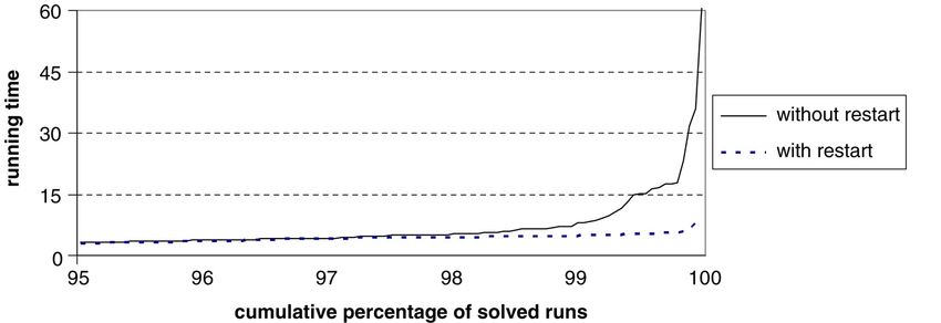
R. Geraerts, M.H. Overmars / Robotics and Autonomous Systems 54 (2006) 165–173                           167

                                                     Fig. 2. The six scenes used for testing.

These are the most crucial steps and they strongly influence the           from the Motion Strategy Library [27]. Furthermore, to make
running time and the structure of the roadmap graph.                       extensive experimentation possible, we did not include huge
   Furthermore, we focus on multiple shot techniques and                   environments such as those common in CAD environments.
will not consider single shot methods such as RRT-based                        cage: This environment consists of many primitives. The
planners [23].                                                             flamingo (7049 polygons) has to find a route (from a few dozen
                                                                           possibilities) that leads him out of the cage (1032 triangles).
3. Experimental setup                                                      The complexity of this environment will put a heavy load on
                                                                           the collision checker but the paths are relatively easy.
    In this study we restricted ourselves to free-flying objects in
a three-dimensional workspace. Such objects have six degrees                   clutter: This scene consists of 500 uniformly distributed
of freedom (three translational and three rotational). In all              tetrahedra. A torus must move among them from one corner to
experiments, we used the most simple local method that                     the other. The configuration space will consist of many narrow
consists of a straight-line motion in configuration space. For             corridors. There are many solutions to the query.
other types of devices or local planners the results might be                  hole: The moving object consists of four legs and must rotate
different. We will investigate this in future work.                        in a complicated way to get through the hole. The hole is placed
    The PRM approach builds a roadmap which, in the query                  off-center to avoid that certain grid-based methods have an
phase, is used for motion planning queries. We aim at                      advantage. The configuration space will have two large open
computing a roadmap that covers the free space adequately but              areas with two narrow winding passages between them.
this is difficult to test. Instead, in each test scene we defined              house: The house is a complicated scene consisting of about
a relevant query and continued building the roadmap until the              2200 polygons. The moving object (table) is small compared
query configurations were in the same connected component.                 to the house. Because the walls are thin, the collision checker
    All techniques were integrated in a single motion planning             must make rather small steps along the paths, resulting in much
system called SAMPLE (System for Advanced Motion                           higher collision checking times. Because of the many different
PLanning Experiments), implemented in Visual C++ under                     parts in the scene the planner can be lucky or unlucky in finding
Windows XP. All experiments were run on a 2.66 GHz                         the relevant part of the roadmap. So we expect a large difference
Pentium 4 processor with 1 GB internal memory. We used Solid               in the running times of different runs.
as the basic collision checking package [37]. In all experiments               rooms: In this scene there are three rooms with lots of
we report the running time in seconds. Because the experiments             space and with narrow doors between them. So the density of
were conducted under the same circumstances, the running time              obstacles is rather non-uniform. The table must move through
is a good indication of the efficiency of the technique. For those         the two narrow doors to the other room.
techniques where there are random choices involved we report                   wrench: This environment features a large moving object
the average time over 30 runs.                                             (156 triangles) in a small workspace (48 triangles). There are
    For the experiments we used the following six scenes                   many different solutions. At the start and goal the object is
(see Fig. 2). The cage and wrench scenes are borrowed                      rather constrained.
168                                R. Geraerts, M.H. Overmars / Robotics and Autonomous Systems 54 (2006) 165–173

4. Collision checking                                                     Table 1
                                                                          Running times for different collision checking methods

     The most time-consuming steps in the probabilistic roadmap                           Collision checking
planner are the collision checks that are required to decide                              incremental        binary           line    rotate-at-s
whether a sample lies in Cfree and whether the motion produced            cage              2.4                 1.9             1.8      2.7
by the local planner is collision-free. In particular the second          clutter           1.8                 1.3             1.4      3.1
type of checks is time consuming. In this section we investigate          hole            431.9               422.3           436.4   1206.7
                                                                          house             6.4                 4.9             4.7     47.1
some techniques for collision testing of the paths.                       rooms             0.5                 0.4             0.4      1.1
     As basic collision checking package we use Solid [37]. The           wrench            0.9                 0.5             0.5      1.1
advantage of this package is that it considers objects like blocks,
tetrahedra, spheres, and cylinders as solids rather than boundary
                                                                             The table shows that in all scenes the binary approach was
representations. This avoids the generations of samples inside
                                                                          faster than the incremental approach although the improvement
obstacles. Also it reduces the number of obstacles required to
                                                                          varied over the type of scene. The line check only had a
describe complicated scenes. Solid builds a data structure based
                                                                          marginal effect, contrary to the claim in [10]. This might be due
on bounding boxes for fast query answering.
                                                                          to the way Solid performs the collision checking with the line
     When testing a path for collisions we can use the following
                                                                          segment. In [10] it was suggested to only apply the line check
techniques.
                                                                          when the distance between the endpoints is large. We tried this
     incremental: In the incremental method we take small steps
                                                                          but did not see any significant improvement in performance.
along the path from start to goal. For each placement we check
                                                                             Also the rotate-at-s technique did not give the improvement
for collisions with the scene.
                                                                          suggested in [1]. It should though be noticed that this can
     binary: In the binary method we start by checking the
                                                                          depend on the underlying collision checking package used. For
middle position along the path. If it is collision-free we recurse        the rest of the paper we will use the binary approach without
on both halves of the path checking the middle positions                  line checks.
there. In this way we continue until either a collision is found
or the checked placements lie close enough together (again                5. Uniform sampling
determined by a given step size) [33].
     In early papers on PRM the incremental method was used.                  The first papers on PRM used uniform random sampling of
Later papers suggest that the binary method works better [34].            the configuration space to select the nodes that are added to the
The reason is that the middle position is the one that has the            graph. In recent years, other uniform sampling approaches have
highest chance of not being collision free. This means that,              been suggested to remedy certain disadvantages of the random
when the path is not collision free, this collision will most likely      behavior. In particular we will study the following techniques.
be found earlier, that is, after fewer collision checks.                      random: In the random approach a sample is created by
     It has been suggested that one should try to compute sweep           choosing random values for all its degrees of freedom. The
volumes and use these for collision tests. As a result, a path            sample is added when it is collision-free.
check would require just one collision test. The problem is                   grid: In this approach we choose samples on a grid. Because
that it is very difficult to compute sweep volumes for three-             the grid resolution is unknown in advance, we start with a
dimensional moving objects with six degrees of freedom. A                 coarse grid and refine this grid in the process, halving the cell
much simpler technique is to first check with the sweep volume            size. Grid points on the same level of the hierarchy are added in
introduced by the origin of the object, that is, with a line              random order.
segment between start and goal position (see [10]).                           Halton: In [7] it has been suggested to use so-called Halton
     line check: In this method we first perform a collision test         point sets as samples. Halton point sets have been used in
with the line segment between the start and goal position in the          discrepancy theory to obtain a coverage of a region that is better
workspace. Only if it is collision-free do we perform the binary          than using a grid (see e.g. [8]). It has been suggested in [7] that
method. (This assumes that the origin of the object lies inside           this deterministic method is well suited for PRM.
it.)                                                                          Halton*: In this variant of Halton we choose a random
     We would expect that this test will quickly discard many             initial seed instead of setting the seed to zero [41]. The claims
paths that have a collision, leading to an improvement in                 in [7] should still hold because they are independent of the seed.
running time.                                                             By choosing a random seed we avoid the situation in which seed
     rotate-at-s: While the previous methods check collisions             zero is lucky or unlucky.
along a straight line, the rotate-at-s approach first translates              random Halton: In this approach we use again Halton
from start to an intermediary configuration s halfway, then               points. But when adding the nth sample point we choose an area
rotates, and finally translates to the endpoint [1]. We set s to          around this point (in configuration space) and choose a random
0.5.                                                                      configuration in this area. As size of the area we choose k A/n
     Table 1 summarizes the results (using deterministic Halton           where A is the area of (the relevant part of) the configuration
points for sampling and a simple nearest-k node adding                    space and k is a small constant. (We set k to 0.2.) So the area
strategy; see below).                                                     becomes smaller when more and more points are added. This
R. Geraerts, M.H. Overmars / Robotics and Autonomous Systems 54 (2006) 165–173 169
Table 2 Table 3
Comparison of average running times of six basic sampling strategies Comparison of average running times of six advanced sampling strategies
Basic sampling strategy Sampling around obstacles
random grid Halton Halton* rnd cell-based Gaussian obstacle obstacle* bridge MA NC Halton*
halt.
cage 7.3 3.1 5.3 3.3 215.9 5.4 2.0
cage 2.3 3.2 1.9 2.0 1.5 2.8 clutter 2.8 2.0 2.6 3.3 620.4 7.1 1.5
clutter 1.2 3.4 1.3 1.5 1.5 1.4 hole 8.8 47.5 7.1 35.4 7.7 2.3 201.4
hole 433.9 370.4 422.3 201.4 435.5 279.5 house 18.0 20.7 13.0 28.8 199.3 15.7 10.4
house 78.7 3.2 4.9 10.4 17.9 10.0 rooms 0.5 0.4 0.5 1.0 3.5 0.4 0.7
rooms 0.7 0.8 0.4 0.7 0.6 0.7 wrench 2.7 0.9 1.9 0.7 11.0 3.8 0.4
wrench 0.7 0.4 0.5 0.4 0.7 0.4
added randomness is another way suggested to solve cases in Gaussian: Gaussian sampling is meant to add more samples
which Halton is unlucky. near obstacles. The idea is to take two random samples,
cell-based: In this approach we take random configurations where the distance between the samples is chosen according
within cells of decreasing size in the workspace. The first to a Gaussian distribution. Only if one of the samples lies in
sample is generated randomly in the whole space. Next we split Cfree and the other lies in Cforb we add the free sample. This
the workspace in 23 equally sized cells. In a random order we leads to a favorable sample distribution [5].
generate a configuration in each cell. Next we split each cell obstacle based: This technique, based on [2], has a similar
into sub-cells and repeat this for each sub-cell. This should lead goal. We pick a random sample. If it lies in Cfree we add it to
to a much better spread of the samples over the configuration the graph. Otherwise, we pick a random direction and move the
space. A similar approach was employed in [32]. sample in that direction with increasing steps until it becomes
An important question is how to choose random values. free and add the free sample.
Random values were obtained by the Mersenne Twister [28]. obstacle based*: This is a variation of the previous
Sampling for the rotational degrees of freedom (S O3) was technique where we throw away a sample if it initially lies in
performed by choosing random unit quaternions [22]. See [42] Cfree . This will avoid many samples in large open regions.
for a more extensive elaboration on sampling methods for S O3. bridge test: The bridge test is a hybrid technique that aims
Table 2 summarizes the results. It can be seen that the results at better coverage of the free space [15]. The idea is to take
were rather varying. In general the differences were small, that two random samples, where the distance between the samples
is, the slowest method took about twice the time of the fastest is chosen according to a Gaussian distribution. Only if both
method. But for each scene another technique was the fastest. samples lie in Cforb and the point in the middle of them lies
There was just one exception. The random approach performed in Cfree is the free sample added. (To also get points in open
reasonable well except in the house scene. For this particular space, every sixth sample is simply chosen randomly.)
scene there was a huge variation in running times between medial axis: This technique generates samples near the
different runs. More that a third of the runs took 6 s or less, medial axis (MA) of the free space [40]. All samples have two
while another third took more than 100 s (one run even took equidistant nearest points resulting in a large clearance from
650 s). As a result, conclusions based on average times are obstacles. The method increases the number of samples in small
difficult to make. Also the other approaches had a high variation volume corridors but is relatively expensive to compute.
in running time. Fig. 3 shows a box plot of the different running nearest contact: This method generates samples on the
times for the rooms scene for the methods. The cell-based boundary of the C-space and can be seen as the opposite to
approach seemed to have the lowest variance. the medial axis technique. First we choose a uniform random
It is interesting to compare Halton and Halton*. In some sample c. If c lies in Cfree we discard it, else we calculate
sense Halton is simply one particular run of Halton*. We saw the penetration vector v between c and the environment. Then
that for example for the house scene it was a lucky run while
we move c in the opposite direction of v and place c on the
for the hole scene it was an unlucky run. Adding a bit of
boundary of the C-space. Care must be taken not to place c
randomness did not seem to remedy this problem.
exactly on the boundary, because then it would be difficult to
In general we must conclude that there is little to win when
make connections between the samples.
using different kinds of uniform sampling in terms of average
We expect these techniques to be useful only in scenes
running time. There can though be other arguments to use
where there are large open areas (in configuration space) and
a particular technique. For example, the Halton approach is
some narrow passages. Table 3 shows the results. (The Halton*
deterministic. Even though it might be unlucky on a particular
scene this still is a favorable property. approach is shown for comparison.)
As expected, the techniques only performed considerably
6. Advanced sampling better for the hole scene. Also for the rooms scene the methods
worked well but the improvement was not significant. However,
Rather than using uniform sampling, it has been suggested in other situations the methods were up to ten times slower.
to add more samples in difficult regions of the environment. In The medial axis approach was even worse, due to the expensive
this section we study a number of these techniques. calculations. The method does though give samples that are170 R. Geraerts, M.H. Overmars / Robotics and Autonomous Systems 54 (2006) 165–173
Fig. 3. Box plot for the rooms scene, showing the variation in running time for 30 runs. A vertical line represents the minimum and maximum value of the
experiments and the box represents the middle fifty per cent of the data.
nicely located between the obstacles, which leads to motions Table 4
with a higher clearance. Comparison between four node adding strategies
We conclude that special non-uniform techniques should Node adding strategy
only be used in specific situation with narrow corridors. nearest-k comp comp-k visibility
Preferably they should also only be used in the parts of the cage 1.9 3.4 1.6 3.0
workspace where this is relevant; see e.g. [18]. clutter 1.3 1.3 1.4 2.3
hole 409.5 7428.2 7554.4 102.5
7. Node adding house 4.9 3.0 13.0 45.5
rooms 0.4 0.2 0.2 6.3
wrench 0.5 0.4 0.4 1.6
In this section we will study how to select the set of
neighbors to which we try to make connections. As each test for
a connection is expensive we should try to avoid these as much We consider the following techniques.
as possible. On the other hand, if we try too few connections we nearest-n: We try to connect the new configuration c to the
will fail to connect the graph. It is not useful (from a complexity nearest n nodes in the graph. The rationale is that nearby nodes
point of view) to make connections to nodes that are already lead to short connections that can be checked efficiently. If
in the same connected component, because a new connection many nearby nodes lie in the same connected component there
will not help solving motion planning queries. Also, it is not is no other component in the neighborhood so it is acceptable
useful to try to connect to nodes that lie too far away. The that we only connect to a single component.
chance of success for such a connection is minimal while the component: We try to connect the new configuration to
collision checks required for testing the path are expensive. An the nearest node in each connected component that lies close
important question here is what we use as a distance measure; enough. The rationale is that we prefer to connect to multiple
see also [1]. In this paper we use d = dt + dr , where dt denotes connected components.
the translational distance of the origin of the object and dr component-n: We try to connect the new configuration to
denotes the rotational distance between two unit quaternions at most n nodes in each connected component. Still we keep
that represent the start and goal orientation; see [22]. This the total number of connections tried small (the same number
measure is easy to compute and gives a reasonable estimate. as for nearest-n). The rationale is that when the number of
We performed a large number of experiments to determine components is small we prefer to spend some extra time on
for each scene the optimal values for the maximal distance trying to make connections. Otherwise the time required for
d and for the maximum number of connections k. It turned adding the node will become the dominant factor.
out that for most test scenes a value of k between 20 and 25 visibility: This method is based on the visibility sampling
was best. Only for the clutter scene a much smaller value of technique described in [30]. We try to connect the new
around 10 was required. The reason is that many connections configuration to useful nodes. Usefulness is determined as
are invalid due to the large number of obstacles. So even when follows: when a new node can be connected to no other nodes
there are many connected components it does not help to try to it forms a new connected component and is labeled useful. If it
connect to them. For the maximal distance a similar argument connects two or more components it is also labeled useful. If it
holds. For large open scenes, like the cage and the wrench, can be connected to just one component it is not labeled useful.
a large value is best. For more constrained scenes, a smaller It has been observed in [30] that the number of useful nodes
value is required. For the hole scene an even smaller value remains small, making it possible to try connections to all of
works best. The reason is that in the difficult part of the scene them.
only short connections have a chance of success. We used the Table 4 summarizes the results. Although the visibility
optimal values in this paper. In general, one would like to have approach pruned the graph a lot, it still performed worse on
a technique that determines the best values based on (local) most scenes. Only for the hole scene did it perform better.
properties of the scene. Such a technique is currently lacking. We feel that the reason is that the approach is too strict inR. Geraerts, M.H. Overmars / Robotics and Autonomous Systems 54 (2006) 165–173 171
Fig. 4. Cumulative percentages of 2000 runs solved in t seconds for the wrench scene.
rejecting nodes. In general, the component-based techniques Table 5
were faster except for the hole scene. We must remark that for Average running times for the wrench scene with and without restarting the
the hole scene it is better to use an obstacle-based sampling PRM
technique such as nearest contact. For this technique, nearest-k Statistics for the variance problem
was actually three times faster than the visibility approach (and minimum average maximum st. dev.
the components techniques). Without restart 0.03 1.01 60.81 2.32
With restart 0.05 0.88 8.20 1.00
8. Variation of running times
An advantage of random sampling techniques is that they random techniques more robust. We plan to investigate this
are usually fast and can successfully deal with the diversity approach further.
of problems. However, a price has to be paid: the running
times needed to find a solution will vary. We noticed that 9. Conclusions
some of them were exorbitantly high, increasing the average
considerably. This phenomenon is undesirable for two reasons. In this paper we have presented the results of a comparative
First, a large variation complicates statistical analysis and can study of various PRM techniques. The results confirm
even make it unreliable. Second, it is undesirable from a user’s previously made claims that the binary approach for collision
point of view; for example, in a virtual environment where real- checking works well. The results showed that many claims
time behavior is required, only a particular amount of cpu time on efficiency of certain sampling approaches could not be
will be scheduled for the motion planner. verified, i.e., there was little difference between the various
A first study of this problem has been reported in [16], uniform sampling methods and they were only outperformed
where a bidirectional A∗ search is used, based on parameterized by advanced sampling methods for special (narrow passage)
formulas for increasing the competence of the local planner. We cases.
propose a new simple technique that can be used to decrease the For node adding it turned out that visibility sampling did not
maximum, average and variance of running times. perform as well as expected. A technique based on choosing a
restart prm: We run PRM for a particular time t. If no number of nodes per component seemed to perform best.
solution is found within t seconds, the PRM is restarted, One thing that is clear from the study is that a careful choice
throwing away the roadmap created so far. We repeat this of techniques is important. Also, it is not necessarily true that
process until a solution is found. Clearly, t should be a a combination of good techniques is good. For example, for
reasonable guess for the time in which we expect that the the hole scene one might expect that a combination of nearest
problem can be solved. If no such guess can be made we can contact and visibility works best. But experiments showed that
also start with a small value and double the time t in each step. this combination is actually about three times worse than the
As an example we apply the approach to the wrench scene. best combination.
To make sure our averages make sense we ran the planner 2000 The study also showed the difficulty of evaluating the quality
times. Fig. 4 shows the percentage of runs that have been solved of the techniques. In particular the variance in the running time
in a particular amount of time. We only show the tail of the chart and the influence of certain bad runs were surprisingly large.
because the heads of the two curves are indistinguishable. We presented a very simple variance killer that seems to be
Only 1% of the runs that were generated without restarting effective. We are though fairly certain that better techniques
had a high running time (between 8.0 and 60.8 s). By restarting exist. This is an interesting topic for further study. This study
the PRM after 4 s this interval was dramatically improved to does not provide a final answer as to the best technique. Further
[4.9; 8.2]. This improvement positively changed the average, research, in particular into adaptive sampling techniques,
maximum and standard deviation of running times, which are will be required for this. Also, further study for other
stated in Table 5. We conclude that restarting the PRM makes robot types such as articulated and car-like robots would be172 R. Geraerts, M.H. Overmars / Robotics and Autonomous Systems 54 (2006) 165–173
interesting since we only compared techniques for free-flying The Algorithmic Perspective. The Third Workshop on the Algorithmic
objects. Foundations of Robotics, 1998, pp. 141–154.
We hope that our studies shed some more light on the [18] D. Hsu, Z. Sun, Adaptive hybrid sampling for probabilistic roadmap
planning, Technical Report TRA5/04, National University of Singapore,
questions of what technique to use in which situation. A major 2004.
challenge is to create planners that automatically choose the [19] L.E. Kavraki, Random networks in configuration space for fast path
correct combination of techniques based on scene properties or planning, Ph.D. Thesis, Stanford University, 1995.
that learn the correct settings while running. [20] L.E. Kavraki, J.-C. Latombe, Randomized preprocessing of configuration
space for fast path planning, in: IEEE Int. Conf. on Robotics and
Automation, 1994, pp. 2138–2145.
Acknowledgements [21] L.E. Kavraki, P. S̃vestka, J.-C. Latombe, M. Overmars, Probabilistic
roadmaps for path planning in high-dimensional configuration spaces,
This work was supported by the Netherlands Organization IEEE Transactions on Robotics and Automation 12 (1996) 566–580.
for Scientific Research (N.W.O.) and by the IST Programme [22] J.J. Kuffner, Effective sampling and distance metrics for 3D rigid body
of the EU as a Shared-cost RTD (FET Open) Project path planning, in: IEEE Int. Conf. on Robotics and Automation, 2004, pp.
3993–3998.
under Contract No IST-2001-39250 (MOVIE - Motion
[23] J.J. Kuffner, S.M. LaValle, RRT-connect: An efficient approach to single-
Planning in Virtual Environments). We would like to thank query path planning, in: IEEE Conf. on Robotics and Automation, 2000,
Dennis Nieuwenhuisen who created part of the SAMPLE pp. 995–1001.
software. [24] F. Lamiraux, L. Kavraki, Planning paths for elastic objects under
manipulation constraints, International Journal of Robotics Research 20
(3) (2001) 188–208.
References [25] J.-C. Latombe, Robot Motion Planning, Kluwer, 1991.
[26] J.-C. Latombe, Motion planning: A journey of robots, molecules, digital
[1] N.M. Amato, O. Bayazit, L. Dale, C. Jones, D. Vallejo, Choosing good actors, and other artifacts, International Journal of Robotics Research 18
distance metrics and local planners for probabilistic roadmap methods, (1999) 1119–1128.
in: IEEE Int. Conf. on Robotics and Automation, 1998, pp. 630–637. [27] S.M. LaValle, Planning Algorithms, http://msl.cs.uiuc.edu/planning,
[2] N.M. Amato, O. Bayazit, L. Dale, C. Jones, D. Vallejo, OBPRM: An 2004.
obstacle-based PRM for 3D workspaces, in: Workshop on the Algorithmic [28] M. Matsumoto, T. Nishimura, Mersenne twister: A 623-dimensionally
Foundations of Robotics, 1998, pp. 155–168. equidistributed uniform pseudorandom number generator, Transactions
[3] N.M. Amato, Y. Wu, A randomized roadmap method for path and on Modelling and Computer Simulation 8 (1998) 3–30.
manipulation planning, in: IEEE Int. Conf. on Robotics and Automation, [29] D. Nieuwenhuisen, M.H. Overmars, Using cycles in probabilistic
1996, pp. 113–120. roadmap graphs, in: IEEE Int. Conf. on Robotics and Automation, 2004,
[4] J. Barraquand, L.E. Kavraki, J.-C. Latombe, T.-Y. Li, R. Motwani, P. pp. 446–452.
Raghavan, A random sampling scheme for path planning, International [30] C. Nissoux, T. Siméon, J.-P. Laumond, Visibility based probabilistic
Journal of Robotics Research 16 (1997) 759–774. roadmaps. in: IEEE Int. Conf. on Intelligent Robots and Systems, 1999,
[5] R. Bohlin, Motion planning for industrial robots. Ph.D. Thesis, Göteborg pp. 1316–1321.
University, 1999. [31] M.H. Overmars, A random approach to motion planning, Technical
[6] R. Bohlin, L.E. Kavraki, Path planning using lazy PRM, in: IEEE Int. Report RUU-CS-92-32, Utrecht University, 1992.
Conf. on Robotics and Automation, 2000, pp. 521–528. [32] B. Salomon, M. Garber, M.C. Lin, D. Manocha, Interactive navigation in
[7] M. Branicky, S. LaValle, K. Olson, L. Yang, Quasi-randomized path complex environments using path planning, in: Symposium on Interactive
planning, in: IEEE Int. Conf. on Robotics and Automation, 2001, pp. 3D Graphics, 2003, pp. 41–50.
1481–1487. [33] G. Sánchez, J.-C. Latombe, A single-query bi-directional probabilistic
[8] B. Chazelle, The Discrepancy Method, Cambridge University Press,
roadmap planner with lazy collision checking, in: Int. Symposium on
Cambridge, 2000.
Robotics Research, 2001, pp. 403–418.
[9] J. Cortes, T. Simeon, J.P. Laumond, A random loop generator for planning
[34] G. Sánchez, J.-C. Latombe, On delaying collision checking in PRM
the motions of closed kinematic chains using PRM methods, in: IEEE Int.
planning — application to multi-robot coordination, International Journal
Conf. on Robotics and Automation, 2002, pp. 2141–2146.
of Robotics Research 21 (1) (2002) 5–26.
[10] L. Dale, Optimization techniques for probabilistic roadmaps. Ph.D.
[35] T. Simeon, J. Cortes, A. Sahbani, J.P. Laumond, A manipulation planner
Thesis, Texas A&M University, 2000.
[11] L. Dale, N.M. Amato, Probabilistic roadmaps – putting it all together, in: for pick and place operations under continuous grasps and placements, in:
IEEE Int. Conf. on Robotics and Automation, 2001, pp. 1940–1947. IEEE Int. Conf. on Robotics and Automation, 2002, pp. 2022–2027.
[12] R. Geraerts, M.H. Overmars, A comparative study of probabilistic [36] P. S̃vestka, Robot motion planning using probabilistic road maps. Ph.D.
roadmap planners, in: Workshop on the Algorithmic Foundations of Thesis, Utrecht University, 1997.
Robotics, 2002, pp. 43–57. [37] G. van den Bergen, Collision Detection in Interactive 3D Environments,
[13] L. Han, N.M. Amato, A kinematics-based probabilistic roadmap method Morgan Kaufmann, 2003.
for closed chain systems, in: Algorithmic and Computational Robotics: [38] P. Švestka, M.H. Overmars, Motion planning for car-like robots,
New Directions. The Fourth Workshop on the Algorithmic Foundations a probabilistic learning approach, International Journal of Robotics
of Robotics, 2000, pp. 233–245. Research 16 (1997) 119–143.
[14] C. Holleman, L.E. Kavraki, J. Warren, Planning paths for a flexible surface [39] P. Švestka, M.H. Overmars, Coordinated path planning for multiple
patch, in: IEEE Int. Conf. on Robotics and Automation, 1998, pp. 21–26. robots, Robotics and Autonomous Systems 23 (1998) 125–152.
[15] D. Hsu, T. Jiang, J. Reif, Z. Sun, The bridge test for sampling narrow [40] S.A. Wilmarth, N.M. Amato, P.F. Stiller, MAPRM: A probabilistic
passages with probabilistic roadmap planners, in: IEEE Int. Conf. on roadmap planner with sampling on the medial axis of the free space, in:
Robotics and Automation, 2003, pp. 4420–4426. IEEE Int. Conf. on Robotics and Automation, 1999, pp. 1024–1031.
[16] D. Hsu, T. Jiang, J. Reif, Z. Sun, On addressing the run-cost variance [41] X. Hickernell, F, J. Wang, Randomized Halton sequences, Mathematical
in randomized motion planners, in: IEEE Int. Conf. on Robotics and and Computer Modelling 32 (2000) 887–899.
Automation, 2003, pp. 2934–2939. [42] A. Yershova, S.M. Lavalle, Deterministic sampling methods for spheres
[17] D. Hsu, L.E. Kavraki, J.-C. Latombe, R. Motwani, S. Sorkin, On finding and S O(3), in: IEEE Int. Conf. on Robotics and Automation, 2004, pp.
narrow passages with probabilistic roadmap planners, in: Robotics: 3974–3980.R. Geraerts, M.H. Overmars / Robotics and Autonomous Systems 54 (2006) 165–173 173
Roland Geraerts received his M.S. degree in Mark Overmars received his Ph.D. degree in
Computer Science in 2001 from Utrecht University Computer Science in 1983 from Utrecht University
in the Netherlands. Currently he is a Ph.D. candidate in the Netherlands. Currently he is a full professor
at the Department of Computer Science at the same at the Department of Computer Science at the same
university. His interests include robotics and motion university. Here he heads the Center for Geometry,
planning. Imaging and Virtual Environments. His main research
interests include computational geometry and its
application in areas like virtual reality, robotics, and
computer games.You can also read