Salish Sea Ambient Noise Study: Best Practices (2021)

Salish Sea Ambient Noise Study: Best Practices
 (2021)

 This work was sponsored and financially supported by the Vancouver Fraser Port Authority. Transport Canada provided
 additional financial support.

 For bibliographic purposes, this document should be cited as follows:

Eickmeier, J., Tollit, D., Trounce, K., Warner, G., Wood, J., MacGillivray, A. and Zizheng Li (2021) Salish Sea Ambient Noise
Study: Best Practices (2021). Vancouver, British Columbia, Vancouver Fraser Port Authority, Enhancing Cetacean Habitat and
Observation (ECHO) Program.

Authors: Justin Eickmeier1, Dominic Tollit2, Krista Trounce3, Graham Warner4, Jason Wood5, Alex MacGillivray6 and Zizheng
Li7

1) Justin M. Eickmeier is a Consulting Scientist at SLR Consulting (Canada) Ltd., Vancouver, British Columbia, V6J 1V4
(jeickmeier@slrconsulting.com)
2) Dominic J. Tollit is the Principal Scientist at SMRU Consulting North America, Vancouver, British Colunbia, V6B 1A1
(djt@smruconsulting.com)
3) Krista B. Trounce is the Research Manager for the ECHO Program, Vancouver Fraser Port Authority, Vancouver, British
Columbia, V6C 3T4 (krista.trounce@portvancouver.com)
4) Graham Warner is a Project Scientist for JASCO Applied Sciences (Canada) Ltd.
5) Jason Wood is Operations Manager & Senior Research Scientist at SMRU Consulting North America
6) Alex MacGillivray is a Senior Scientist for JASCO JASCO Applied Sciences (Canada) Ltd.
7) Zizheng Li is a Project Scientist for JASCO JASCO Applied Sciences (Canada) Ltd.

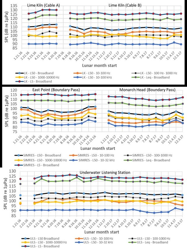
Table of Contents
Abstract ............................................................................................................................................................................................. 2
 Introduction .............................................................................................................................................................................. 3
 Ambient Noise ...................................................................................................................................................................... 4
 Noise Monitoring in the Salish Sea ...................................................................................................................................... 6
 Ambient Noise Evaluation Project (Best Practices) ........................................................................................................... 10
 Hydrophone systems .......................................................................................................................................................... 12
 1) Hydrophone systems - Summary of findings ................................................................................................................. 12
 Calibrations:............................................................................................................................................................................. 12
 Sensitivity: ............................................................................................................................................................................... 12
 System noise: ........................................................................................................................................................................... 13
 Flow-noise: .............................................................................................................................................................................. 14
 2) Hydrophone systems – Discussion and contemporary studies ....................................................................................... 15
 3) Hydrophone systems – key recommendations ............................................................................................................... 17
 Location: .................................................................................................................................................................................. 17
 Equipment: .............................................................................................................................................................................. 17
 Calibration: .............................................................................................................................................................................. 18
 System monitoring:.................................................................................................................................................................. 18
 Vessel Traffic ..................................................................................................................................................................... 19
 1) Vessel Traffic - Summary of findings ............................................................................................................................ 19
 2) Vessel traffic - Discussion and contemporary studies .................................................................................................... 22
 3) Vessel traffic - key recommendations ............................................................................................................................ 24
 Large vessel traffic .................................................................................................................................................................. 24
 Environmental Factors........................................................................................................................................................ 25
 1) Environmental Factors – summary of findings .............................................................................................................. 25
 Wind and rain: ......................................................................................................................................................................... 25
 Tidal currents: .......................................................................................................................................................................... 26
 Sound speed profile: ................................................................................................................................................................ 27
 Biologicals: .............................................................................................................................................................................. 29
 2) Environmental factors - discussion and contemporary studies....................................................................................... 29
 3) Environmental factors - key recommendations .............................................................................................................. 31
 Data Analysis and Reporting Metrics ................................................................................................................................. 32
 1) Data Analysis and Reporting Metrics – summary of findings ....................................................................................... 32
 2) Data Analysis and Reporting Metrics- discussion and contemporary studies ................................................................ 34
 3) Data analysis and reporting - key recommendations ...................................................................................................... 36
 Conclusion .......................................................................................................................................................................... 37
Acknowledgments ........................................................................................................................................................................... 40
References ....................................................................................................................................................................................... 41

 1

ABSTRACT

All monitoring locations and hydrophone systems have unique features that affect the ability to monitor

ambient noise levels accurately. As anthropogenic underwater noise effects on marine species becomes

increasing important globally, it is imperative to understand how best to consistently measure, analyze, and

account for factors contributing to the soundscape. The Enhancing Cetacean Habitat and Observation

Program, led by the Vancouver Fraser Port Authority, seeks to mitigate shipping noise effects on at-risk

whales, particularly endangered Southern Resident Killer Whales. Utilizing two years of data from three

different, cabled inshore hydrophone stations in the Salish Sea, this high-level review aims to help understand

and address key environmental and anthropogenic factors that contribute to ambient noise. Contributions

from: the hydrophone system and ancillary equipment; rain, wind and tidal currents; factors affecting sound

propagation; biological presence; and vessel traffic are considered in this study, and “best practice”

recommendations for undertaking standardized long-term noise assessment are provided. Key findings

highlight that early and frequent quality assessment protocols are imperative, weather and tidal information

should be collected proximate to the hydrophone, vessel traffic was the dominating influence at all locations

across all measured frequencies, and validated noise models should augment empirical data collection.

Monthly variability in sound pressure levels was 2-6 dB, highlighting the analytical challenges in determining

“existing” conditions and detecting trends or testing mitigation strategies. Accounting for the key factors

contributing to the soundscape is considered critical in these evaluations.

 Index Terms Acoustic signal processing, Best practices, Environmental factors, Oceanography, Remote

monitoring, Underwater acoustics, and Underwater technology.

 2

INTRODUCTION

The Vancouver Fraser Port Authority’s (the port authority’s) Enhancing Cetacean Habitat and Observation

(ECHO) Program is a port authority-led collaborative program aimed at better understanding and managing

the cumulative effects of shipping activities on at-risk whales throughout the southern coast of British

Columbia. The ECHO Program is guided by the advice and input of a volunteer advisory working group and

associated technical committees, with representatives from Canadian and American government agencies,

the marine transportation industry, Indigenous communities, conservation and environmental groups, naval

architects, engineers, and scientists.

 One of the priorities of the ECHO Program is to develop mitigation measures leading to quantifiable

reductions in underwater noise (UWN) caused by marine shipping, which the Department of Fisheries and

Oceans Canada (DFO) Recovery Strategy identifies as one of the key threats to the recovery of the Southern

Resident Killer Whales (SRKW). Therefore, quantifying the potential noise benefits of different mitigation

strategies, developing an understanding of existing ambient noise conditions, and what factors most affect

ambient noise is crucial.

 In 2015, under the guidance of the ECHO Program’s Acoustic Technical Committee (ATC), the program

initiated an ambient noise monitoring project in the Salish Sea. An inland sea of the Pacific Ocean, the Salish

Sea is located in British Columbia, Canada and Washington State, USA. It includes the Strait of Georgia,

Strait of Juan de Fuca and a network of connecting channels. The primary purpose was to consistently

measure ambient underwater acoustic levels, over two years, at three representative locations to:

 • Establish existing underwater ambient noise levels regionally at key reference sites.

 • Ground truth and better calibrate regional-level acoustic models.

 • Establish trends in underwater noise levels regionally and temporally to facilitate on-going and

 adaptive underwater noise management in the future.

 • Investigate the effectiveness of mitigation measures implemented by the ECHO Program or others.

 3

This document summarizes the findings of the “Ambient Noise Evaluation Project,” [1] which evaluated

two years of ambient noise level data collected from the three reference sites using standardized reporting

protocols developed by the ATC. It provides guidance and recommendations on collecting and analyzing

ambient noise data in the Salish Sea.

 AMBIENT NOISE

 The ECHO program focuses on assessing mitigation of underwater noise caused by marine shipping, a

known threat to the recovery of endangered SRKW. To measure and understand how effective any noise

reduction mitigation measure might be, requires a full understanding of variability and the accuracy of

empirical measurements, and the factors that contribute or confound those measurements.

 In 1962, Wenz published an early study on ambient noise, identifying three primary sources: the effects of

surf, rain, hail, tides (or water motion), anthropogenic sources such as ships, and biological sources

(crustaceans, fish, and marine mammals). Wentz suggested that future studies of ambient noise should

consider temporal (hourly, daily, and seasonal) and spatial (directional) measurements [2]. Talham studied

the directional distribution of ambient noise and found the noise field to be anisotropic but indicated no

existing theory accounted for energy from a single source arriving at the same terminal location over multiple

paths [3]. Urick classified ambient noise under two categories, based on directional properties. Type I noise

(low-frequency) arrived at all hydrophones on a vertical array with high coherence and no time delay.

Anthropogenic noise from distance vessels is the primary source of this noise. Type II noise originated at the

sea surface and was the dominant high-frequency noise source when wind speeds are high [4].

 In 1970, Perrone determined ambient noise levels to be a function of water depth, frequency, and wind

speed in the Northwest Atlantic. Calibration of the hydrophone and data acquisition system was an integral

component of this study [5]. By 1981, Wagstaff had determined the study of ambient noise to be a complex

 4

phenomenon requiring both the interpretation of measurements and an understanding of acoustic propagation

theory [6].

 In the 1990s, the monitoring and modeling of ambient noise were studied (concerning a three-dimensional

ocean environment), and consideration in the design and placement of hydrophones for in situ measurements

improved acoustic propagation modeling [7]. Existing concepts on ambient noise's directionality expanded

to include range-dependent environments and focused on the attenuation effects of upslope and downslope

propagation [8].

 In 2009, the study of ambient noise in the ocean was advanced significantly by Hildebrand through an

extensive investigation into anthropogenic and natural noise sources. Frequency bands were used to classify

noise sources: low (10 to 500 Hz), mid (500 Hz to 25 kHz), and high (above 25 kHz) [9]. Anthropogenic

sources such as commercial vessel traffic or seismic surveys dominated the low-frequency noise band.

Oceanographic and meteorological processes such as breaking waves, sea spray, bubble formation/collapse,

and rainfall contributed to the mid-frequency band. Small vessels also contributed to ambient noise in the

mid-frequency band. Hildebrand identified small vessels as having peak energy at 5 kHz when operated at

speeds between 10 to 20 knots. At high frequencies, propagation loss confines all noise sources to an area

close to the receiver. Hildebrand identified four critical environmental factors that influence acoustic

propagation and the measurement of ambient noise levels: I) measurement of the sound speed profile, II)

attenuation properties of seawater, III) local bathymetry and IV) the properties of bottom sediment layers [9].

 The above studies are standard references for contemporary investigations (2010-2020) on ambient noise.

Contributions from Merchant et al., (2012), Dekeling et al., (2014) and MacGillivray et al., (2018) [10-12]

(amongst other studies discussed in this document) reported overall ambient noise levels and individual

contributions from anthropogenic, biological, and environmental sources. These studies and guides set the

groundwork for this best practices document.

 5

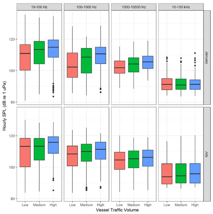
Figure 1: Ambient noise monitoring stations in the Salish Sea (2016-2017).

 NOISE MONITORING IN THE SALISH SEA

 The ECHO Program ambient noise evaluation project included collecting two years of ambient noise data

from key reference locations within the Salish Sea. Three existing cabled hydrophone sites were selected to

represent three sub-areas of the Salish Sea in proximity to the commercial shipping lanes (Fig. 1). Based on

the Acoustic Technical Committee’s advice, two years of data was recommended as the minimum timeframe

to evaluate existing ambient noise conditions and describe any clear trends. Calibrated hydrophones in Haro

Strait (Lime Kiln) and Boundary Pass (East Point and subsequently nearby at Monarch Head) were deployed

in shallow water (23-30 m depth) in critical SRKW habitat, between one and five kilometers from the

 6

shipping lanes, noting the ATC considered a depth of less than 20 m to be sub-optimal for monitoring low-

frequency ambient noise bands. The hydrophone in the Strait of Georgia, termed underwater listening station

(ULS), was deployed in deeper water (173 m) and precisely positioned between the northbound and

southbound shipping lanes to accurately measure source levels of transiting Automated Identification System

(AIS) equipped vessels while also collecting ambient noise data.

 Acoustic data from these three sites were collected for approximately two years (2016-2017), noting a

relatively small location change (East Point to Monarch Head) at Boundary Pass in year two. The East Point

hydrophone was operational from January 2016 until March 2017. The Monarch Head hydrophone was

operational during all of 2017 [1]. Each location has a unique soundscape based on local bathymetry,

environmental characteristics, anthropogenic contributions, and source-receiver geometry. Furthermore, the

data acquisition hardware for each hydrophone system varied between sites. In 2015, Dakin and Heise

provided a pertinent regional review of hydrophone system installation decisions for various scenarios,

including choice of location, depth and hydrophone system specifications, and recommendations for post-

processing techniques [13].

 The review of underwater noise monitoring guidance documents [10,11,14] subsequently led the ECHO

Program’s ATC to develop an initial standardized sampling, analysis, and reporting scheme for long-term

ambient noise measurements. The results of that work, summarized in Table 1, governed the data collection

and standardized analysis protocols. It is important that the precise definition of the frequency bands used in

the ECHO study be specified, as different conventions can be encountered in the literature. All frequency

bands used by the Program are distributed on a logarithmic scale and are based on powers of ten around a

reference frequency of 1000 Hz. The lower and upper frequency limits of the decade bands are:

(Eq. 1) = 1000 ∙ 10 

(Eq.2) = 1000 ∙ 10( +1) , = −2, −1, 0, …

 7

where the lower frequency limit of the first decade band starts at 10 Hz and the upper frequency limit of the

highest decade band is truncated at the maximum sampling frequency.

 For a finer resolution, the center frequencies of nominal 1/3-octave bands (which are, by convention, one-

tenth decade bands) are constructed by multiplying the reference frequency by 10(n/10), with n = –20

corresponding to a center frequency of 10 Hz. The lower and upper frequency limits for any of these bands

goes from:

 ( −0.5)
(Eq.3) = 1000 ∙ 10 10 , to
 ( +0.5)
(Eq.4) = 1000 ∙ 10 10 , ≥ −20

 For example, for the center frequency of 100 Hz (n = −10) the band limits are 89.125 Hz and 112.20 Hz.

Although the more formal qualifier for these bands is decidecade as per the ISO 18405 standard [15], the

combined bandwidth of three contiguous decidecade bands is approximately one octave, and for this reason

some standards still refer to them as “1/3-octave” bands [16]. This traditional terminology is used in the

ECHO analyses.

 8

TABLE I

 ECHO PROGRAM ANALYSIS AND REPORTING SCHEME (2017)

 Factor Proposed Rationale

Temporal 2 years of reference measurements, analysis, Considered the minimum period to collect reference ambient

sampling and review. noise data.

Data sampling Lunar month, with analysis of weekly and “Standardize” platform flow noise across comparative periods,

blocks daily rhythms. given the difficulties in removing platform flow-noise due to

 tidal current effects.

Fundamental Power Spectral Density (PSD): (dB re 1 PSD and SPL are both standard ambient noise reporting metrics.

reporting metrics µPa2/Hz)

 Sound Pressure Levels (SPL): (dB re 1 µPa)

Bandwidth 10 Hz–100 kHz This frequency bandwidth range captures acoustic energy from

 vessels, as well as SRKW communication and echolocation

 bands.

PSD reporting Percentile exceedance PSD plots (1-minute Percentile PSD plots are useful for comparison across regional

protocols average) sites and interpreting noise sources and system noise.

 Annotated PSD spectrogram plots (1-hour

 average) Long-term spectral averages or spectrograms allow the

 interpretation of temporal noise cycles (diurnal and tidal) and

 identification of dominant acoustic sources (natural and

 anthropogenic).

SPL reporting SPL reporting in broadband, decade band, To provide summary noise data using metrics suitable for

protocols and 1/3-octave bands (re 1μΡa, 1-minute universal comparison and in frequency bands relevant to

 average) with consideration to SRKW SRKW.

 specific communication and echolocation

 frequency bands. At the time of the 2017 study, no universal reporting metrics

 were identifiable in peer-reviewed publications or international

 SPL, in the form of exceedance percentiles, guides. Given the evolving nature of this field of study, a range

 9

including median (L50), min., max., quartiles of metrics were considered.

 (L25 and L75), and using the arithmetic mean

 (Leq) of the squared sound pressure.

 System Full calibration (at the start of each study) Maintain high-quality data collection.

 performance and and regular in situ system checks, consisting

 data quality of high dynamic range and sensitivity gain

 checks.

 Auxiliary data Environmental auxiliary data includes: Key local influencing factors.

 needs weather, current speed, and sound

 propagation conditions. For anthropogenic

 sources, vessel movement patterns.

 AMBIENT NOISE EVALUATION PROJECT (BEST PRACTICES)

 In 2018, the ECHO Program’s ATC met to review the processed dataset from the 2016-2017 ambient

noise monitoring project and plan a study to identify key factors that require further investigation when

evaluating ambient noise trends and applied mitigation efforts. The ECHO Program subsequently initiated

the ambient noise evaluation project to seek answers to the following questions:

 1. What were the temporal variabilities and trends in ambient noise (across both broadband and finer-

 scale frequency bands) for each site, and did these hold for all three sites?

 2. What key factors and trends (if any) affected ambient noise differences and variability at each site?

 3. What are the critical requirements for future monitoring of ambient noise (i.e., including system

 performance, resolution, and methods for data analysis) to best understand the contribution of

 commercial vessel traffic to ambient noise levels?

 10

The generalized approach began with defining factors that influence ambient noise levels in these

complex and heavily trafficked inshore waters. The following factors were deemed to require additional

study to determine how they contribute to underwater ambient noise levels at each site:

 • Hydrophone systems and data quality (system noise, sensitivity range, and calibration)

 • Vessel traffic

 • Weather and tidal conditions

 • Sound speed profile (SSP) and associated variability in acoustic propagation

 • Biological (animal) presence

 Dekeling et al. recommended consideration of sea state, wave height, water and air temperature,

proximity to marine nature reserves, wrecks, and military sites as well as other nearby permanent

anthropogenic noise sources (e.g., gas pipeline, wind farm, fish farm) for evaluation of ambient noise [11].

These factors (except for water temperature used in the calculation of sound speed) were not evaluated in

the ECHO Program study, noting that evaluation of wind speed was conducted as a suitable proxy metric

for sea state and wave height.

 Given the ECHO Program’s focus on SRKWs (considered a high-frequency odontocete) [17] it was

essential to distinguish how these factors affect different frequency bands; therefore, a decade band

analytical approach was taken. In the low-frequency band (10-100 Hz, 1 decade), vessel noise dominates

the soundscape. In higher frequency decade bands (0.1-1 kHz, 1-10 kHz, and 10-100 kHz), killer whale

vocalizations occur and hearing abilities peak.

 For each of the influencing factors identified for this region, the following sections describe the factor, a

high-level summary of findings from the ECHO Program’s ambient noise evaluation project, a discussion

of how other studies have considered this factor, and recommendations or best practices for measurement

and evaluation in the Salish Sea based on findings from the ECHO Program, and key guidance formulated

from other studies.

 11

Hydrophone systems

1) Hydrophone systems - Summary of findings

 A hydrophone system’s performance relates to how a data acquisition system affects measured levels of

underwater ambient noise: including consideration of system noise, hydrophone sensitivity, frequency range,

and calibration. In the ambient noise evaluation project, aural and visual methods allowed system noise

assessment after hydrophone calibration. All three sites are cabled systems, run independently and

consequently utilized different hydrophones and systems. System noise was unique to each recording system;

however, contamination of data from narrow-band tones and electrical power supplies was identifiable at all

study sites. Some system noises varied with time, but others were consistent. All sites had low-pass anti-

aliasing filters, which affected the detection of quiet sounds at high frequencies. At East Point, a site that

relied on solar power, system noise was substantial and frequently present in all decade bands (Fig.2). Using

such heavily “contaminated” data to establish existing conditions is not recommended without careful

consideration of additional filtering needs. Forced redactions due to naval activity occurred in some months

at the ULS, resulting in loss of data in the lower frequency decade bands.

Calibrations:

 All three sites used high quality calibrated hydrophones, but calibration methods varied. The pistonphone

calibrations made at Lime Kiln found no loss of sensitivity at 250 Hz, whereas, at Monarch Head, a high-

frequency calibration error biased the 10–64 kHz decade band levels.

Sensitivity:

 The sensitivity of hydrophones at all sites met ECHO Program requirements and ranged between -165 and

−171 dB re 1 V/μPa, well within recommended sensitivity levels for this type of monitoring [11].
 12

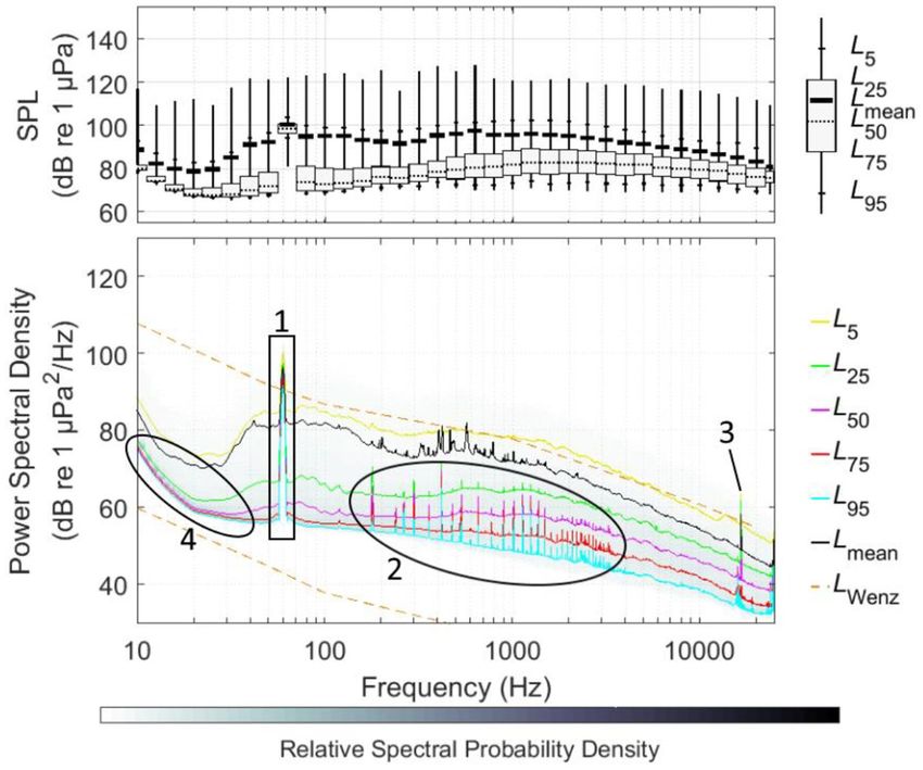
System noise:

 A review of PSD exceedances identified several system noise issues. The effects of these varied across

sites and were more substantial during quiet periods (e.g., nighttime, no vessels present, slack tide, low wind),

including; electrical noise spikes at both low and high frequencies, unwanted noise from GPS, and an acoustic

Doppler current profiler (ADCP). East Point (Fig. 2) had a significant power supply spike at 60 Hz with

harmonics extending to 3800 Hz. Autonomous deployments may reduce certain aspects of system noise

generally associated with cabled external power supplies.

 13

Figure 2: Example of notable data quality issues identified using 1/3-octave bands and power spectral density

levels recorded from 22 Jan 2016 to 21 Feb 2016 (East Point) with four annotated system noise features

identified. Annotation 1 shows the 60 Hz power supply tone. Annotation 2 shows harmonics from the power

supply tone. Annotation 3 shows tones from a solar panel feeding the power grid. Annotation 4 shows the

low-frequency noise floor [1].

Flow-noise:

 Currents in the study area are predominantly tidally driven, with typical peak flow speeds ranging between

0.5-1.0 m/s at ebb and flood. Tidal currents can produce substantial flow noise on the hydrophone and

mooring components, with effects documented at 10–100 Hz levels during high-current periods. At such

 14

times, this noise limited a recorder’s ability to measure low levels of low-frequency sounds. Site comparisons

were not possible due to the lack of local current data at Lime Kiln and East Point.

2) Hydrophone systems – Discussion and contemporary studies

 In 2016, Merchant et al. suggested that consistency in the monitoring instrumentation, sensor placement,

and continuity of the time series have a strong influence on the statistical power of passive monitoring

programs and that shallower bathymetry results in comparatively poor acoustic propagation, attenuating the

contribution of shipping noise [18]. ACCOBAMS (The Agreement on the Conservation of Cetaceans of the

Black Sea, Mediterranean Sea and contiguous Atlantic area) suggested that long-term hydrophone stations

should be placed in high and low traffic areas and near oceanographic stations. In addition, a recent sonar

survey of local bathymetry is recommended for hydrophone deployment and subsequent analysis (with

emphasis on hydrophone deployment sites in deep water with low current speeds) [19].

 In 2014, Robinson et al. wrote a “Good Practice Guide for Underwater Noise Measurement” on behalf of

Marine Scotland. This guide provided direction on noise measurements and identified commonly used

metrics for describing underwater noise, including definitions and units. The recommendations included

reporting metrics and guidance on hydrophone selection, data acquisition systems, and calibration

procedures. For shallow water deployments, the measuring hydrophone ideally resides in the lower half of

the water column, between half and three-quarters of the total depth (measured from the sea surface). In very

shallow water, the variation in tidal depth may significantly affect sound propagation [14].

 Dekeling et al. recommended that calibration should include the full frequency range of interest for the

specific application at hand, noting that it is possible to calibrate a hydrophone and recording system with an

overall uncertainty of less than 1 dB [11].

 Dakin and Heise suggested that hydrophone calibrations take place at least once every two years.

Calibration facilities provide a higher degree of accuracy (± 0.5 to ± 2 dB) than in situ calibrations (± 3 to ±

 15

6 dB) but are more labor and time-intensive. It is tempting to set the system gain high to detect distant or low

amplitude sounds on recording systems with adjustable gain. However, this also amplifies the system's self-

noise and can cause louder sounds to saturate the hydrophone, and the combination reduces the dynamic

range of the system. System noise can be associated with the pre-amplifiers, filters, and power supplies in

the data acquisition system. Also, cables, moorings, and anchoring systems may add to the noise of a

hydrophone installation. The use of a shroud, installed over the hydrophone element, is recommended, and

decoupling the hydrophone from the mooring using a shock cord can also help to dampen noise, including

fauna noise on the mooring, such as crabs and fish [13]. Kinda et al. also highlighted flow noise as an issue

for autonomous moorings and suggested flow noise effects might be minimized by reporting (low-frequency)

results only for periods of low current flow [20].

 The Joint Monitoring Programme for Ambient Noise in the North Sea (JOMOPANS) issued a 2018 report

on “Standard procedure for equipment performance, calibration, and deployment”. The report also

recommended calibration for any hydrophone and recording system deployed for the study of ambient noise.

Ideally, hydrophone calibrations should occur in the same mounting configuration and temperature/depth,

which the hydrophone is likely to experience in the field. Prior to deployment and following the recovery,

field calibrations are essential to ensure no significant changes in the hydrophone response occur throughout

the deployment. The recommended frequency range for calibrations should, at a minimum, cover the

frequencies of interest between 10 Hz and 20 kHz [21].

 Flow noise contamination can reduce the correlation between broadband shipping noise and the frequency

bands used as anthropogenic noise indicators, making these indicators less effective. Since flow noise

increases with decreasing frequency, lower frequency bands are more affected, particularly the 63 Hz band

used for the European Commission Marine Strategy Framework Directive [18].

 In 2015, the Baltic Sea Information on the Acoustic Soundscape (BIAS) report stated that system-noise is

a key consideration when measuring low amplitude signals. Expression of self-noise as a spectrum level,

either in µV/Hz at the amplifier input or back-calculated as µPa/Hz at the hydrophone, should be at least 6

 16

dB below the lowest noise level of interest [22]. To minimize random and systematic uncertainties, quality

controls were implemented throughout the processing steps by testing the signal processing software and

performing inter-organization comparisons (ring tests) of the signal processing methodologies.

3) Hydrophone systems – key recommendations

 Based on the learnings of the ECHO Program ambient noise evaluation project and a review of other

relevant studies, the following points represent best practices for hydrophone systems and data quality:

Location:

 Hydrophone sampling should be conducted at the same location and depth, year-over-year, to confidently

establish long-term trends. Consistency is particularly crucial for near-shore hydrophones, which can be

substantially affected by bathymetric features and shorelines blocking noise sources.

Equipment:

 Where possible, the use of cabled systems for long term monitoring is advantageous. This allows for

continuous data collection (no duty cycle required) at wide bandwidth and on-going system performance

checks. A minimum water depth of 20 - 30 m is recommended for any installation.

 If possible, utilize identical systems at all monitoring locations if looking to characterize a regional

soundscape. If this is not possible, select systems with similar performance (sampling rate, bit-rate, and anti-

aliasing filters). Installation of shrouds to help reduce biofouling (in addition to reducing flow noise) and a

ready supply of system components to ensure timely replacement (if a failure occurs) is pragmatic.

 17

Calibration:

 Characterization of a hydrophone and recording system's response curve should ideally be within ±1 dB

over the full frequency range of interest (e.g., 10 Hz to 100 kHz). End-to-end system calibrations should be

spot-checked, at minimum, annually (using a pistonphone or other controlled sound source) to ensure no

long-term variations in the recording system's sensitivity. Where possible, different recorders should be co-

located during calibration, allowing for comparison of ambient noise measurements and characterization of

system noise.

System monitoring:

 Before deployment, measurement of the hydrophone’s noise floor (1-minute PSD spectrum) in a quiet

laboratory setting is preferable. After deployment, the noise floor (1-minute PSD spectrum) of the

hydrophone and recording system should be measured monthly during a quiet period. Interfering noise

sources should be identified in situ, if possible.

 Undertake regular aural checks on data quality (unusual noises, reduced performance). Catalogue and

ideally fix any underlying data quality issues (Fig. 2). Identifying residual data quality issues is preferable in

early data post-processing (to allow filtering or analytical remedies).

 Monthly reviews of measured 1-minute 1/3-octave band noise levels are suitable for monitoring changes

in system noise characteristics. Any significant changes in system noise characteristics require investigation,

as they may indicate impending system failure (e.g., increased low-frequency noise may be associated with

water ingress into hydrophone electronics).

 Consistently record all system specifications and all modifications (e.g., gain settings, maintenance

operations, calibration events) that occur between deployments.

 18

Vessel Traffic

1) Vessel Traffic - Summary of findings

 Vessel movement patterns at all three ECHO Program reference sites made use of AIS data. Additional

small boat (non-AIS) information was collected from photographic evidence at East Point and by an

acoustic detector at Lime Kiln.

 Vessels were the dominating factor affecting ambient noise levels at all three sites and across all

frequencies considered. Large AIS vessel presence dominated noise levels between 10-100 Hz and was also

a significant contributing factor at higher frequencies. This mirrors published sources in the Salish Sea [23],

especially for sites close to the shipping lane [18]. Fig. 3 (below) shows a density plot of vessel traffic

hours versus distance from the hydrophone at each study site. In Haro Strait, the peaks at 2.5 and 4.5 km

from the Lime Kiln hydrophone correspond to the inbound and outbound international shipping lanes,

respectively. The peak in the Boundary Pass density plot, 2 km from the East Point / Monarch Head

hydrophones, was due to vessel traffic in both the inbound and outbound shipping lanes. A spike in the

density plot around 6.25 km from the ULS in the Strait of Georgia was primarily due to tug traffic entering

and exiting the Fraser River [1].

 19

Figure 3: Density plot of vessel traffic hours versus distance from the hydrophone at each site [1].

 When reviewing sound pressure level (SPL) statistics, the arithmetic mean (Leq) values were below the L5

values but well above (>10 dB) the L50 (median SPL) at all sites, which indicated that short-term, high-

amplitude noise sources were present (such as large vessels). The ULS, adjacent to the shipping lane, had

the highest monthly mean ambient noise sound pressure levels (Leq = 119.8 dB re 1µPa). Lime Kiln, the

site furthest from the shipping lanes, had the highest monthly median ambient noise levels (L50 = 108.4 dB

re 1µPa), and experienced regular, close proximity transits of small boats [1].

Fig. 4 (below) shows the influence of traffic volume from large commercial vessels at Lime Kiln. Low,

medium, and high-volume traffic days were determined from daily large commercial vessel traffic hours in

the 0-25th, 25th-75th, and 75th-100th percentiles, respectively. At Lime Kiln, hourly sound levels increased

 20

with vessel traffic in the first three-decade bands (especially in January), but increases in the fourth decade

band (10-100 kHz) were either smaller (July) or negligible (January).

Figure 4: Box-and-whisker plots of hourly decade-band sound levels (Lime Kiln) versus large commercial

traffic volume in January (top) and July (bottom) 2017 [1]. A box-and-whisper plots illustrates the center,

spread, and overall range of data from a visual 5-number summary. The top and bottom of the box are the

upper and lower quartiles (25th and 75th percentiles), while the horizontal line is the median (50th

percentile). Whiskers (vertical lines) indicate the lower extreme and upper extreme values within 1.5 x the

interquartile range. Black dots indicate outliers.

 Small (non-AIS) vessels in close proximity to the hydrophone can dominate the soundscape, as found at

Lime Kiln (Fig. 5). Overall, at this site small vessels were found to dominate some higher frequencies. Fig.

 21

5 compares SPL cumulative distribution functions when no vessels were detected, when large vessels were

acoustically detected, when large vessels were detected by AIS, and when small vessels were acoustically

detected. The large vessel acoustic detector was in good agreement with AIS detections above an SPL of

115 dB re 1µPa. Divergence at lower levels is driven by false negatives (missed detections of distant

vessels).

Figure 5: SPL cumulative distribution functions (Lime Kiln) with broadband (10 Hz to 100 kHz) 1-minute

cumulative exceedance probability plots for January (left) and July (right) 2017, during periods with

acoustic detections of large vessels (dark blue), small vessels (pink), and no-vessels (red). SPLs for times

when there were AIS transmissions within 6 km of the hydrophone are shown in cyan [1].

2) Vessel traffic - Discussion and contemporary studies

 Studies focused on vessel noise typically only report ambient noise levels at lower frequencies where

large vessels are known to be significant contributors [9]. Vessel noise effects have thus often focused on

baleen whales that are considered a low-frequency hearing group. However, more recent regional studies

have highlighted elevated median background levels associated with vessel presence at low frequencies
 22

(20-30 dB from 100 to 1,000 Hz) and higher frequencies (5-13 dB from 10,000 to 96,000 Hz). Thus, noise

received from commercial vessels at ranges less than 3 km extends to mid-frequencies used by odontocetes,

such as killer whales, for communication and echolocation [24]. Typically, noise from small boats peaks at

higher frequencies than larger ocean-going commercial vessels. Managing underwater noise, as part of the

European Union’s “Marine Strategy Framework Directive” (MSFD), has resulted in a focus on measuring

annual mean (Leq) continuous noise (such as that emitted by large commercial vessels) levels in just two

1/3-octave bands centered at 63 and 125 Hz.

 Several subsequent publications and reports have extended reporting frequencies, especially to higher

frequencies (e.g., 2 kHz), mainly to take better account of the frequencies in which key large cetaceans

vocalize, as well as suggesting alternative or additional reporting metrics [10, 18, 19]. Consequently, in

addition to annual mean estimates, reports of cumulative distribution functions (CDF, Fig. 5) of SPL are

recommended by many of the more recent European reports and papers reviewed (see further discussion in

Data Analysis and Reporting Metrics section). This CDF approach permits the concurrent visualization of

multiple SPL dB exceedance metrics. In a recent SRKW noise effect study in the Salish Sea [25], a CDF

approach was used to generate monthly cumulative noise distribution maps. Merchant et al. undertook a

systematic review of different noise metrics and concluded that L10 or L5 is the most appropriate for

tracking anthropogenic noise levels in the marine environment, as these high dB exceedance metrics are

most sensitive to intermittent high noise levels typically caused by vessel transits [18].

 All reviewed contemporary ambient noise studies highlighted the need to access AIS information on

shipping movements as AIS data provide information on vessel density and proximity to monitoring

locations, as well as vessel speed and class [18, 25]. Such factors are considered necessary in understanding

trends in ambient noise levels. Only a small fraction of private pleasure crafts, fishing vessels, and

ecotourism boats are equipped with AIS transponders, yielding an underestimation of these vessels' actual

contribution to noise levels. In some inner coastal waters, noise from motorized recreational (non-AIS)

vessels can elevate 1/3-octave band noise centered at 0.125, 2, and 16 kHz by 47–51 dB [26] and dominate

 23

the soundscape. In areas of known high density non-AIS recreational traffic, understanding these vessel’s

contributions are essential when interpreting ambient noise levels and generating cumulative noise models.

Multiple studies also recommend considering auxiliary environmental data when assessing the influence of

vessel noise on ambient noise levels (see Environmental Factors section below).

3) Vessel traffic - key recommendations

 Based on the learnings of the ECHO Program ambient noise evaluation project and a review of other

relevant studies, the following points represent best practices for collecting and analyzing AIS and non-AIS

vessel movements:

Large vessel traffic

 Continuous traffic monitoring using a land-based AIS receiver located near the hydrophone is preferable.

Periods with AIS receiver outages require identification and AIS data quality checks (e.g., vessel type) to

help ensure data consistency. Additional factors such as vessel proximity to the hydrophone, vessel

type/size, and vessel speed are necessary for detailed analyses.

 Transits of non-AIS vessel traffic should be monitored at the hydrophone location, using a combination

of acoustic and non-acoustic methods to increase the detection rate. Results from this study suggest that a

combination of camera and hydrophone-based detections may be an effective method. Alternative

monitoring methods, such as radar, may also be useful for monitoring non-AIS vessels.

 Utilizing vessel source levels [27], combined with AIS and other tracking data to model the noise field of

both AIS and non-AIS vessels, is also recommended for a fulsome evaluation of ambient noise

contributions across larger areas, as well as to explore mitigation efficacy [28].

 24

Environmental Factors

1) Environmental Factors – summary of findings

 Environmental factors that influence ambient noise belong to three broad categories: weather and tides,

sound speed profile variability, and the presence of biological noise sources.

 Wind creates breaking waves and can elevate ambient noise levels during quiet periods when vessel noise

is negligible. It also increases high-frequency transmission loss due to rough sea surface-induced scattering

and weakened coherent reflections. The sound of rainfall may be detected at the hydrophone, particularly

for shallow installations.

 Variation in the refractive properties of the SSP influences the path of acoustic propagation. Refraction

occurs due to changes in sound speed, which is a function of temperature, pressure, and salinity. Sea-

surface roughness, bathymetry, and seabed composition (e.g., sand, silt, and clay) also affect sound

propagation. These characteristics of the water column, surface, and seafloor are critical inputs for accurate

modeling and developing a robust understanding of acoustic propagation at a particular monitoring site.

 Biological presence relates to underwater sounds generated by marine fauna, such as marine mammal

vocalizations and echolocation clicks, that affect ambient noise.

 In combination with a predictive ocean current model and local current measurements (where available),

local weather station data allows evaluation of how wind, rain, and tidal currents may have affected

ambient noise data.

Wind and rain:

 Seasonal changes in wind-induced ambient noise (>100 Hz) were identifiable at Lime Kiln and East

Point for winter conditions but not during summer conditions. Rainfall events in this study made negligible

contributions to ambient noise levels at each site. Ideally, to better understand the acoustic impact of

rainfall, data should be collected close to the hydrophone location and on a fine (e.g., 1-minute) timescale.

 25

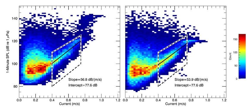
Tidal currents:

 At the ULS, ADCP measurements allowed for better characterization of flow noise from tidal currents

(Fig. 6); however, the high-frequency chirps of the ADCP also contaminated the acoustic recordings. With

current data from a predictive tidal model, correlations were less distinct at Lime Kiln and East

Point/Monarch Head. Low-frequency system noise at East Pont also limited the ability to interpret tidal

effects. Mechanical or electromagnetic current meters located proximate to the hydrophone deployment

may be preferable for future ambient monitoring.

Figure 6: ULS correlation analysis to assess current speed effects on noise levels. Sound pressure levels

(SPL; 1-minute average) in the 10–100 Hz decade band as a function of water current speed were compared

for January (left) and July 2017 (right). Linear regressions (solid black lines) were fit to the data within the

dashed line, indicating a positive correlation effect above 0.4 m/s [1].

 26

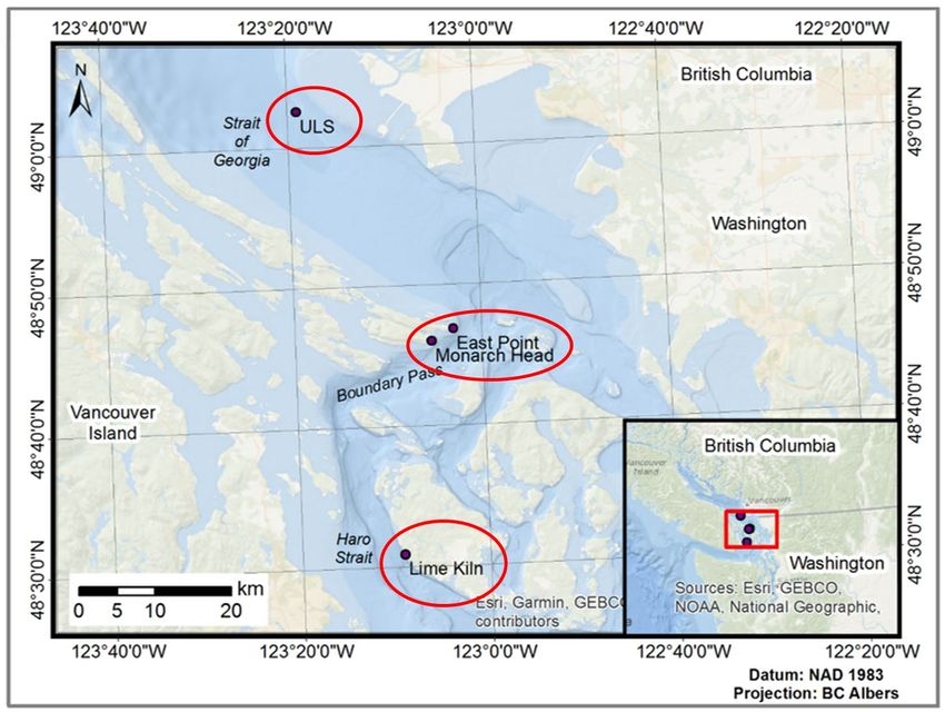
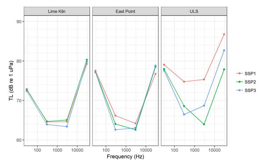
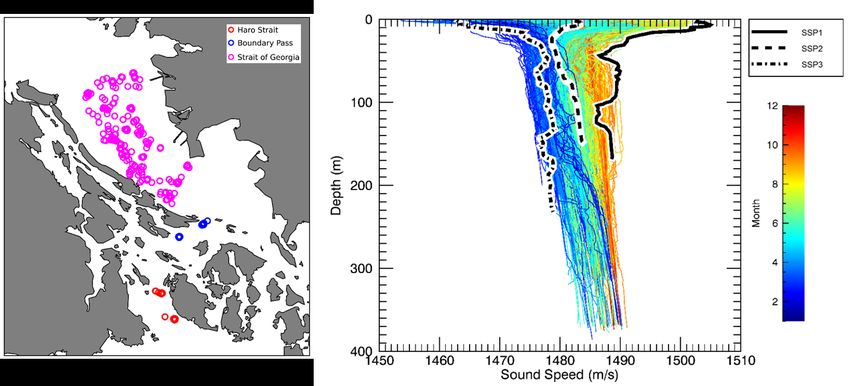
Sound speed profile:

 SSP measurements in the Salish Sea showed more seasonal variations at the ULS than either Lime Kiln

or East Point; however, greater temporal and spatial coverage of SSP measurements at that location may

have played a factor (Fig.7).

Figure 7: Map (left) showing sound speed profile (SSP) measurements locations in the Salish Sea (circles)

[29]. Sound speed profiles measured in the Strait of Georgia (right). SSP profiles 1, 2, and 3 (summer,

fall/spring, and winter) represent the observed range of SSP variability at this site. The sound channels at

~50 and 120 m will not have a large effect on transmission loss between shallow noise sources (e.g., ships

and waves) and the hydrophone at 170 m depth [1].

 SSP measurements were used with wind speed measurements and seabed properties to model acoustic

propagation at each site (Fig. 8). Propagation modelling, used JASCO’s Marine Operations Noise Model

(MONM) that incorporates the following site-specific environmental properties: I) a bathymetric grid of the

modeled area II) underwater sound speed as a function of depth, and III) a geo-acoustic profile based on the

seafloor's overall stratified composition. MONM computes acoustic fields in three dimensions by modeling

 27

transmission loss within two dimensional (2-D) vertical planes aligned along radials covering a 360° swath

from the source [1].

Figure 8: Average transmission loss (TL) for Lime Kiln (left), East Point (middle), and ULS (right) for a

near-surface source between 2 and 4 km range along a radial between the international shipping lanes and

the hydrophone. Line colors represent the seasonality of sound speed profiles (SSPs), used for modelling

(red: summer, green: fall or spring and blue: winter). Measured seasonal profiles were unique to each site

[1].

 Sound propagation modeling showed that propagation loss was lowest for the mid frequencies, 300 and

3000 Hz and higher during summer (downwards-refracting) conditions. Despite this, ambient noise levels

were higher in summer at all three reference sites, indicating traffic volumes (higher in summer) played a

more important role than the seasonal effects of SSP.

 28

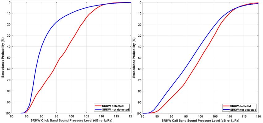
Biologicals:

 The effect of biological presence was analyzed by comparing sound levels at times with and without

(immediately before and after) acoustic detections of marine mammals. Sounds from biological sources are

automatically detected using PAMGuard software and subject to verification by a human analyst. This

evaluation focused on Lime Kiln where there were sufficient periods of confirmed SRKW vocalizations to

conduct an assessment. Biological presence from SRKW increased sound levels in the 1-10 kHz and 10–

100 kHz frequency range by approximately 3 and 7 dB, respectively (Fig. 9).

Figure 9: Lime Kiln: One-minute cumulative exceedance probability plots for periods with and without

Southern Resident Killer Whale (SRKW) detections for “vocalization” decade band SPL (1-10 kHz) (left)

and SRKW “click” decade band SPL (10-100 kHz) [1].

2) Environmental factors - discussion and contemporary studies

 29

A “soundscape” is formally defined by ISO [30] as the “characterization of ambient sound in terms of its

spatial, temporal and frequency attributes, and the types of sources contributing to the sound field”. In

2018, Ainslie described the Atlantic Deepwater Ecosystem Observatory Network (ADEON) project’s focus

on establishing an acoustical/environmental observation network to support baseline measurements and

predictive modeling of the soundscape. This report adds that the ISO definition for soundscape does not

include many “region-specific” sources: system noise, noise from turbulent flow (flow-noise) or surface

gravity waves, nor emissions from vessels or biologicals. The ADEON study includes these sources to

facilitate compatibility between inter-study soundscapes and those studied by other researchers and

institutions [30]. ADEON also focused on biological sources and commercial vessel detection. The regional

detection of biological sources ranged from Fin whales to dolphins.

 Garrett et al. assessed ambient noise with an environmental focus on seasons, wind, and wave height in

Falmouth Bay, UK. The study found that improved propagation conditions in winter may be contributing to

the observed louder average sound levels during this season. Increasing wave height significantly affects

the 63 & 125 Hz 1/3-octave band levels likely contributing to increased noise levels with increasing wave

height in winter. A site-specific environmental evaluation accounts for these natural contributions to local

sound levels [31].

 Dekeling et al. stated that it is beneficial to record any relevant auxiliary data and correlate it with the

measured noise levels during analysis. If auxiliary data must be measured locally, this may require the

deployment of additional equipment. Relevant auxiliary data may include sea-state, wind speed (and

associated measurement height), rate of rainfall and other precipitation (including snow), water depth and

tidal variations across that depth range, water/air temperature, hydrophone depth in the water column, GPS

locations of hydrophones and recording systems, seabed properties, profiles of conductivity, and

hydrostatic pressure as a function of depth [11].

 30

3) Environmental factors - key recommendations

 The monitoring of wind and rain data should occur near the hydrophone location. Wind speed, wind

direction, and precipitation should be recorded on a 1-minute basis, if possible. Wind data is ideally

measured at a standard elevation (a mast 10 m above sea level is recommended).

 A current meter (mechanical, electromagnetic, or acoustical) preferably records water currents' speed and

direction near the hydrophone. In combination with 1-minute SPL data, a linear correlation defines the

relationship between current speed and flow-induced noise (Fig. 6). Acoustical meters require sufficient

separation from the hydrophone to minimize noise contamination. The amount of noise contamination

depends on the current meter (e.g., frequency, power, and beam pattern), recorder (e.g., sample rate and

frequency response), and transmission loss. Determining an appropriate separation distance to minimize

acoustic contamination may require acoustic modelling and test measurements. Electromagnetic meters

require periodic maintenance to clean biofouling. Consideration of fairings, shrouds, and other noise

reduction methods for moorings is recommended.

 Sampling of temperature and salinity profiles should, at minimum, be seasonal (ideally monthly) and

near the hydrophone. Recent storm events and freshwater outflow from major river systems affect

previously measured profiles, so their influence requires consideration. Transmission loss modelling should

use seasonal SSPs to better quantify location-specific and seasonal variability in underwater sound

propagation.

 For assessing the influence of biologicals (marine mammals and fish), automatic acoustic detectors, with

a portion manually validated, should be run on the data. Comparing “quiet times” with and without marine

mammal detections is optimal to evaluate biological sources' potential contribution. Aural review of

acoustic data during quality assurance protocols will help identify other critical biological contributors.

 31