Using machine learning on new feature sets extracted from 3D models of broken animal bones to classify fragments according to break agent
←
→
Page content transcription
If your browser does not render page correctly, please read the page content below
Using machine learning on new feature sets extracted
                                              from 3D models of broken animal bones to classify
                                                     fragments according to break agent *
arXiv:2205.10430v1 [cs.CV] 20 May 2022

                                                  Katrina Yezzi-Woodley†                  Alexander Terwilliger‡                Jiafeng Li ‡
                                                  Eric Chen §           Martha Tappen¶               Jeff Calder ‡          Peter J. Olver‡

                                                                                            Abstract
                                                    Distinguishing agents of bone modification at paleoanthropological sites is at the root of
                                                much of the research directed at understanding early hominin exploitation of large animal re-
                                                sources and the effects those subsistence behaviors had on early hominin evolution. However,
                                                current methods, particularly in the area of fracture pattern analysis as a signal of marrow
                                                exploitation, have failed to overcome equifinality. Furthermore, researchers debate the repli-
                                                cability and validity of current and emerging methods for analyzing bone modifications. Here
                                                we present a new approach to fracture pattern analysis aimed at distinguishing bone fragments
                                                resulting from hominin bone breakage and those produced by carnivores. This new method
                                                uses 3D models of fragmentary bone to extract a much richer dataset that is more transparent
                                                and replicable than feature sets previously used in fracture pattern analysis. Supervised ma-
                                                chine learning algorithms are properly used to classify bone fragments according to agent of
                                                breakage with average mean accuracy of 77% across tests.

                                             Keywords— machine learning, taphonomy, zooarchaeology, bone fragment, marrow exploitation, frac-
                                         ture pattern analysis, hominin-carnivore interactions, subsistence, paleoanthropology, replicability, trans-
                                         parency

                                         1     Introduction
                                         Analyses of bone surface modifications and fracture patterns form the basis of substantial research focus-
                                         ing on early hominin subsistence patterns pertaining to the use of large animal food resources (i.e., meat
                                            * We would like to thank the National Science Foundation NSF Grant DMS-1816917 and the University of Min-
                                         nesota’s Department of Anthropology for funding this research. JC was partially supported by an Alfred P. Sloan
                                         Research Fellowship and a McKnight Presidential Fellowship. Source code to reproduce all experimental results is
                                         available here: https://github.com/jwcalder/MachineLearningAMAAZE.
                                            † Department of Anthropology, University of Minnesota, yezz0003@umn.edu (corresponding author)
                                            ‡ School of Mathematics, University of Minnesota
                                            § Wayzata High School, Plymouth, Minnesota
                                            ¶ Department of Anthropology, University of Minnesota

                                                                                                1
and marrow). These methods are used to identify the agents of bone modification for the purpose of as-
certaining the primary accumulating agent of zooarchaeological assemblages, exploring hominin-carnivore
interactions, and determining hominin access order (i.e., hunting versus various forms of scavenging) (e.g.
Bartholomew & Birdsell, 1953; Binford, 1981, 1984, 1985; Binford, Bunn, & Kroll, 1988; Binford et al.,
1985, 1986; Blumenschine, 1986, 1988, 1989, 1995; Blumenschine et al., 1987; Blumenschine & Cavallo,
1992; Blumenschine, Cavallo, & Capaldo, 1994; Blumenschine & Selvaggio, 1991; Bunn & Ezzo, 1993;
Bunn et al., 1986; Dominguez-Rodrigo, 1997; Domínguez-Rodrigo, 2002; Domínguez-Rodrigo & Barba,
2007; Domínguez-Rodrigo, Pickering, Semaw, & Rogers, 2005; Marean, Spencer, Blumenschine, & Ca-
paldo, 1992; Pante, Blumenschine, Capaldo, & Scott, 2012; Pante et al., 2012; Plummer & Bishop, 2016;
Pobiner, 2015; Potts, 1983; Selvaggio, 1994a, 1994b, 1998; Shipman, 1983, 1986). These long-standing
debates are founded on the premise that the use of large animal food resources was a highly influential
factor in our evolution. Conversely, Barr, Pobiner, Rowan, Du, and Faith (2022) downplayed the role of
meat consumption altogether, stating that there is no evidence for increased carnivory after the appearance
of Homo erectus. Clearly, debates continue on the extent to which large animal food resources informed our
evolutionary past.
     We have been unable to resolve these debates because bone surface modifications and fracture patterns
are subject to equifinality which has not been overcome due to the limitations of current methods. This
is only exacerbated by concerns over inter- and intra-analyst error and intense disagreement among re-
search groups about the validity of currently used methods (e.g. Domínguez-Rodrigo, Saladié, et al., 2017;
Domínguez-Rodrigo et al., 2019; Harris, Marean, Ogle, & Thompson, 2017; James & Thompson, 2015;
Merritt, Pante, Keevil, Njau, & Blumenschine, 2019). Improving methods and ensuring that they are repli-
cable could resolve long-standing debates over early hominin subsistence patterns at important paleoanthro-
pological sites such as Dikika (Domínguez-Rodrigo, Pickering, & Bunn, 2010, 2011, 2012; McPherron et
al., 2010; Thompson et al., 2015) and FLK Zinj (see Domínguez-Rodrigo, Bunn, & Yravedra, 2014; Pante et
al., 2012; Pante, Scott, Blumenschine, & Capaldo, 2015; Parkinson, 2018, and citations contained therein).
     Recently, Thompson, Carvalho, Marean, and Alemseged (2019) hypothesized that scavenging for in-
bone nutrients may have led to the origin of the Human Predatory Pattern, whereby humans hunt animals
larger than themselves. If this is the case, then marrow exploitation may factor into major changes that
happened during the Late Pliocene (3.6 − 2.6 Ma) and the Early Pleistocene (2.6 − 1.8 Ma), such as the
first appearance of our genus Homo (Bobe & Wood, 2021; Du, Rowan, Wang, Wood, & Alemseged, 2020),
the first appearance of stone tools (3.3 Ma) and their subsequent technological advancements (Díez-Martín
et al., 2015; Harmand et al., 2015), and geographic expansion (Prat, 2018; Zhu et al., 2018). Thompson
et al. call for the development of new approaches and lines of analysis as a necessary step to successfully
address these questions. Overcoming current methodological limitations has the potential to open avenues
for advancing our understanding of the evolutionary implications of large animal food resource use on our
genus, Homo.
     In response to current methodological challenges, especially as they pertain to resolving equifinality and
improving replication, researchers have developed and are continuing to develop various methods for analyz-
ing bone surface modifications and fracture patterns through approaches such as geometric morphometrics
(e.g. Arriaza et al., 2017; Courtenay, Huguet, Gonzalez-Aguilera, & Yravedra, 2019; Courtenay, Yravedra,
Huguet, et al., 2019; Courtenay, Yravedra, Mate-González, Aramendi, & González-Aguilera, 2019; Maté-
González, Courtenay, et al., 2019; Palomeque-González et al., 2017; Yravedra, Aramendi, Maté-González,
Austin Courtenay, & González-Aguilera, 2018; Yravedra et al., 2017), confocal profilometry (e.g. Braun,
Pante, & Archer, 2016; Gümrükçu & Pante, 2018; Pante et al., 2017; Schmidt, Moore, & Leifheit, 2012), and
other digital data extraction methods (e.g. Bello, Verveniotou, Cornish, & Parfitt, 2011; O’Neill et al., 2020;
Yezzi-Woodley et al., 2021). Many of these new methods rely on digital imaging, in particular 3D scan-
ning, which has become another prominent avenue of research (e.g. Maté-González, González-Aguilera,

                                                      2
Linares-Matás, & Yravedra, 2019; Yezzi-Woodley, Calder, Olver, Sweno, & Siewert, n.d.) within the field.
     The incorporation of digital imaging and data extraction opens opportunities for using powerful com-
putational tools such as machine learning which has been employed in bone modification studies (Arri-
aza, Aramendi, Maté-González, Yravedra, & Stratford, 2021; Byeon et al., 2019; Cifuentes-Alcobendas &
Domínguez-Rodrigo, 2019; Courtenay et al., 2020; Courtenay, Huguet, et al., 2019; Courtenay, Yravedra,
Huguet, et al., 2019; Domínguez-Rodrigo, 2019; Domínguez-Rodrigo & Baquedano, 2018; Domínguez-
Rodrigo, Fernández-Jaúregui, Cifuentes-Alcobendas, & Baquedano, 2021; Domínguez-Rodrigo, Wonmin,
et al., 2017; Jiménez-García, Abellán, Baquedano, Cifuentes-Alcobendas, & Domínguez-Rodrigo, 2020;
Jiménez-García, Aznarte, Abellán, Baquedano, & Domínguez-Rodrigo, 2020; Moclán, Domínguez-Rodrigo,
& Yravedra, 2019; Moclán et al., 2020; Pizarro-Monzo & Domínguez-Rodrigo, 2020). However, most of
these papers have focused on the use of machine learning for discriminating bone surface modifications.
     The purpose of this paper is to investigate the application of machine learning methods as a means of
classifying 3D meshes of bone fragments using new feature sets. Our collection of fragments consists of
cervid appendicular long bones, that were broken either by hominins, using hammerstone and anvil, or by
carnivores, specifically spotted hyenas. The 3D meshes were created using computed tomography (CT)
and the Batch Artifact Scanning Protocol (Yezzi-Woodley et al., n.d.). We introduce new feature sets that
provide more detailed information about each bone fragment and thus are more useful for distinguishing
agents of bone breakage, and offer more precise data extracted in a highly replicable manner using the
virtual goniometer (Yezzi-Woodley et al., 2021), Mesh Lab (Cignoni et al., 2008) and Python (Van Rossum,
Guido and Drake, Fred L., 2009). A small set of qualitative features were also incorporated in the data.
Together, these data were input into machine learning algorithms to classify each fragment based on the
agent of breakage.
     We trained machine learning classification models in two different ways. First, we trained the classi-
fiers to classify individual breaks, which we call break-level classification, and the fragment prediction is
given by majority voting of the breaks for that fragment. The models are evaluated by their accuracy at
classifying fragments, not individual breaks. Second, we trained classifiers to classify the fragments di-
rectly, allowing the machine learning algorithm to determine the best way to combine information from the
individual breaks. The classification accuracy for the break-level classifiers were only slightly higher than
one could expect from random chance (57.18% − 66.16%). On the other hand, the classification rates of the
fragment-level classifiers, which incorporate the entire ensemble of breaks associated with each fragment,
were substantially improved (72.82% − 79.27%) into a statistically meaningful range.
     Moclán et al. (2019) published the first paper to apply machine learning to distinguish agents of bone
breakage using fracture pattern data (Moclán et al., 2019). They reported near perfect classification rates (≥
98◦ ) for some of their testing models. However, we identified several aspects of concern regarding the data
they used, the way in which they used it, and their failure to follow basic machine learning protocols. First,
there were inconsistencies in the manner in which the data were recorded. Furthermore, it appears that they
bootstrapped their sample prior to splitting it into training and test sets; moreover, they based their analysis
on global, fragment-level variables, but split the sample at the break-level, which is not permitted in a proper
application of machine learning analysis because there are several breaks per fragment. Handling the data
in these ways has the effect of contaminating the training set with data from the test set which, in turn, can
falsely inflate success rates in classification. As we discuss in detail in Section 4, these errors effectively
invalidate their published results. We revisit the Moclán et al. (2019) analysis using both proper machine
learning protocols, and, for illustrative and explanatory purposes, their inappropriate use of bootstrapping
and global variables, thereby reproducing the latter misleading and overly optimistic results. We also provide
the results of an experiment on randomized data showing that both bootstrapping and break-level train-test
splits can arbitrarily inflate accuracy, in many cases up to 100%, even when no information is present in the
dataset.

                                                       3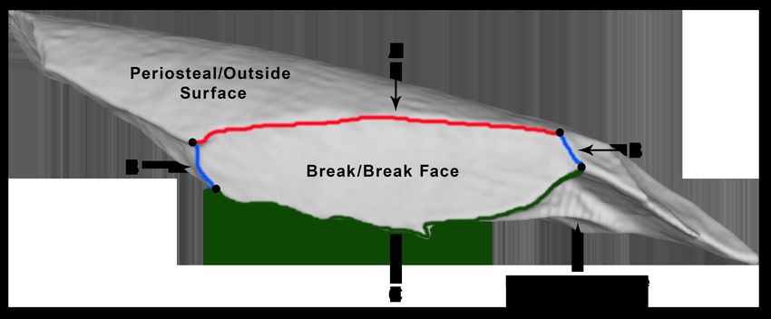
When used correctly, machine learning is a powerful tool that has the potential for advancing approaches
for analyzing bone modifications and subsequently improving our understanding of early human evolution.
Here we demonstrate that using richer data that capture more information about the features from individual
breaks – more than has ever been captured before – offers better discriminatory power. These methods can be
easily replicated by independent research teams. By comparing our application of machine learning to that
of Moclán et al. (2019) we exemplify the ways in which machine learning can be used effectively. Finally,
we argue that classifying fragmentary bone produces higher success rates when both global, fragment level
and local, break level features are used. The ability to classify individual bone fragments holds promise for
improving the resolution with which paleoanthropological sites can be interpreted and furnishes more useful
information for interpreting our evolutionary past.

2     Materials and Methods
2.1    Our Experimental Sample
Our experimental sample (see Table 1) consisted of 463 bone fragments (3,218 breaks) from appendicular
long bones (humeri, radius-ulnae, femora, tibiae, and metapodia) that were derived from Cervus canadensis
(elk) (n = 399 fragments) and Odocoileus virginianus (white-tailed deer) (n = 64 fragments). Previous
researchers have concluded that metapodia are not as useful for distinguishing agents of bone breakage
(Capaldo & Blumenschine, 1994) but this is specific to fracture angles on notches as measured by a contact
goniometer. Given that we used new feature sets and the more precise virtual goniometer (Yezzi-Woodley
et al., 2021), we chose to include metapodia.

                                   Table 1: Our Experimental Sample

                                            HSAnv            Crocuta crocuta                  Total
                                 Fragments (Breaks)      Fragments (Breaks)      Fragments (Breaks)
      Cervus canadensis                    275 (1651)                124 (987)              399 (2638)
        FEM                                 63 (390)                 71 (534)               134 (924)
        HUM                                 28 (159)                 27 (241)                55 (400)
        MTPOD                               71 (409)                     0 (0)               71 (409)
        U NIDENT LBSF                           0 (0)                   2 (15)                  2 (15)
        RAD-ULNA                            38 (243)                  13 (96)                51 (339)
        TIB                                 75 (450)                 11 (101)                86 (551)
      Odocoileus virginianus                     0 (0)                64 (580)                64 (580)
        MTPOD                                   0 (0)                64 (580)                64 (580)
      Total                                275 (1651)              188 (1567)               463 (3218)
    Abbreviations: femur (FEM), humerus (HUM), metapodial (MTPOD), unidentified long bone shaft fragment
    (Unindent LBSF), radius-ulna (RAD-ULN), tibia (TIB), hammerstone and anvil (HSAnv).

    Of the 463 fragments, 275 (1,651 breaks) were produced by hominins and 188 (1,567 breaks) were
produced by carnivores. Hammerstone and anvil were used to break the bones for the hominin sample. The
carnivore sample was created by Crocuta crocuta (spotted hyenas) at the Milwaukee County Zoo (Wiscon-
sin) and the Irvine Park Zoo in Chippewa Falls (Wisconsin). In some instances, articulated limbs were fed
to the hyenas which resulted in two fragments that could not be identified to skeletal element. (See Coil,
Tappen, & Yezzi-Woodley, 2017, for details regarding the experimental protocols.)

                                                     4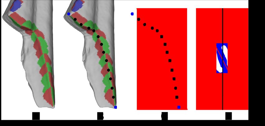
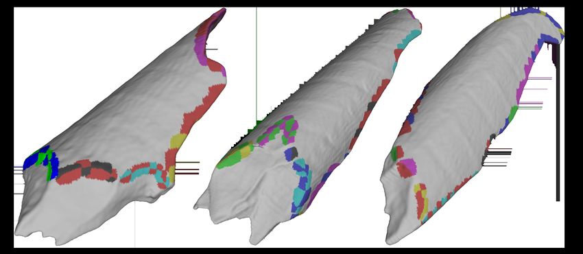
Figure 1: Fragment Features
             Fracture (or break) ridges are used to delineate individual breaks. One fracture
             ridge separates the natural outside surface of the bone from the break surface (A)
             Two ridges on either side of the break serve as boundaries between adjacent breaks
             (B). The interior fracture ridge separates the break from the natural interior surface
             of the bone and, in some cases, other breaks (C).

    Fragments were scanned via computed tomography (CT) using the streamlined Batch Artifact Scanning
Protocol (Yezzi-Woodley et al., n.d.) that we developed to acquire 3D models of each of the fragments,
which were stored as .ply files. Data were extracted from the 3D models of the bone fragments manually
through the Graphical User Interface in Meshlab and automatically using Python scripts.
    To know how each feature was extracted from the fragments, it is important to understand how we
defined the features and in particular how we differentiated breaks, because, as researchers have previously
acknowledged, identifying breaks is not always a straight forward task (Biddick & Tomenchuk, 1975; Bunn,
1982, 1989; Davis, 1985; Pickering, Domínguez-Rodrigo, Egeland, & Brain, 2005). As Bunn (1982, p.43)
points out, the boundary between breaks is neither well-defined nor is it always obvious. Given a long bone,
there is the natural outside (periosteal) surface of the bone and the natural inside (endosteal) surface of the
bone. Fragments from broken long bones also have surfaces that expose what is referred to as breaks or
break faces. Each break is surrounded by fracture (or break) ridges. One of those ridges constitutes the
boundary between the periosteal surface and the break surface for that break (see Figure 1A). Two of the
ridges connect adjacent break faces (see Figure 1B). The fourth ridge is the boundary between the break
face and the endosteal surface of the bone fragment(see Figure 1C). In cases where the break face overlaps
another break face(s) without extending through the entire thickness of the bone, the fourth ridge serves as
a boundary between this break and the more internal break(s) (see Figure 2). Break curves can be extracted
from those ridges (see Figure 3). In more complicated scenarios, the boundary of the break face may contain
additional ridges of various types. It should be noted that ridges are not always easily detectable and one
must decide at which scale to accept a ridge as a boundary and break surface as a separate face. Given
the precision of the tools we used to extract data, we were able to accept small breaks as separate breaks.
Though further discussion is necessary in the field to standardize the definition of an individual break, the
extraction methods used here provide sufficient detail in the data to begin such research.
    Angle measurements were taken along the exterior fracture ridge of each break on each fragment with
the virtual goniometer (Yezzi-Woodley et al., 2021) using radii between 1 − 3 using geodesic distance based
on the size of the break (See Figure 4). When an angle measurement is taken, a colorized patch appears
on the mesh. The center of subsequent angle measurement was placed on the fracture ridge at the border
of the colorized patch indicated by the previous angle measurement. Therefore, measurements were 1 − 3

                                                       5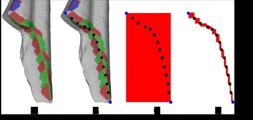
Figure 2: The Interior Ridge
             The interior edge of some breaks border the endosteal surface (A) while others
             border another break (B).

geodesic units apart. When shifting to the next break, the patch colors change (see Figure 5). The endpoints
of each break were chosen using the “Picked Points” tool in Meshlab. The angle and endpoint data were
used to calculate the arc angle (see Figure 6) and break length variables (see Figure 7).
    Additional variables were collected manually through observation of the models such as the presence or
absence of notches (see Figure 8) or trabecula. We ran the models through a Python script to extract more
global features such as the mesh volume and surface area. Data were recorded and calculated for each break,
referred to here as break level data, and for the entire fragment, referred to here as fragment level data. A
summary of these variables are as follows:

Break Level Variables:
   1. Number of Angles: This refers to the number of fracture angle measurements per break. Fracture an-
      gle measurements were taken along each break curve. A minimum of one fracture angle measurement
      was recorded for each break. Type: natural number

   2. Angle data: Because more than one angle measurement could be taken on each break curve, sum-
      mary statistics were calculated for the angle measurements. This included the minimum, maximum,
      mean, median, standard deviation, and range. Type: continuous

   3. Interior Edge: If the interior ridge of the break face transitioned to another break face it was cate-
      gorized as "break". If it adjoined the endosteal surface, then it was categorized as "endosteal" (see

                                                     6
Figure 3: Break Curves
         Break (or fracture) curves can be extracted from the fracture ridges surrounding a
         break face. These break curves correspond to the break ridges illustrated in Figure
         1. The exterior curve separates the periosteal surface from the break surface (A)
         Two curves separate the break from adjacent breaks (B). One curve is the interior
         break curve (C).

         Figure 4: Angle Measurements Along Ridge
         Angle measurements were taken along the entire fracture ridge between the natu-
         ral outside surface of the bone and the break surface.

   Figure 2). Type: Boolean

4. Interrupted: This is a TRUE/FALSE variable indicating whether or not the break curve was inter-
   rupted by another break. Type: Boolean

5. Ridge Notch: If the fracture ridge exhibited the arcuate indentation characteristic of a notch, then the
   break was classified as "TRUE" (see Figure 8A). Type: Boolean

6. Interior Notch: If the interior ridge of the break face exhibited the arcuate indentation(s) character-
   istic of a notch(es), then the break was classified as "TRUE" (see Figure 8B). Type: Boolean

7. Break Lengths: Two measures of break length were recorded. We calculated the Euclidean distance
   between the two endpoints of the break curve (see Figure 7C). When using the virtual goniometer, the
   location of each angle measurement is automatically recorded. Using those points in conjunction with
   the endpoints, we calculated the arc length of each break curve (see Figure 7D). Type: continuous

                                                  7
Figure 5: The Virtual Goniometer Captures More Detail
The virtual goniometer makes it possible to capture more information with a
higher degree of detail. This includes the ability to measure small breaks. When
transitioning from one break to the next, the colors of the patches where the angle
measurements are taken change.
Figure 6: Arc Angle
For each break curve (A) the x−, y−, and z − coordinates for both the endpoints
(blue circles) and the locations of each angle measurement (black points) were
recorded (B). The points were used to define a best fit line (C). The angle between
the best fit line and the principal axis of the fragments was recorded (D).
8. Arc Angle: This is a calculation that we used in lieu of break plane, as defined by Gifford-Gonzalez
(1989). We did this by calculating a best fit line to the ordered points along the break curve and then
calculating the angle between the best fit line and the principal axis of the bone fragment. Again, the
points were taken from the selected endpoints and the virtual goniometer data (see Figure 6). Type:
continuous
8Figure 7: Break Lengths
For each break curve (A) the x−, y−, and z − coordinates for both the endpoints
(blue circles) and the locations of each angle measurement (black points) were
recorded (B). The straight line (Euclidean) distance was measured between the
endpoints of the break curve (C) and the arc length was measured using all the
points (D).
Fragment Level Variables:
1. Number of Breaks: We recorded the number of break faces per fragment. Type: natural number
2. Trabecula: If there was trabecular bone on the fragment it was categorized as "TRUE". Type:
Boolean
3. Volume: The volume of the domain bounded by the surface mesh was extracted in Python. Type:
continuous
4. Surface Area: The surface area of the mesh was extracted in Python. Type: continuous
5. Bounding Box Dimensions: The bounding box dimensions were extracted using Python. This can
be thought of as the fragment length, width, and depth. Type: continuous
6. Angle Data: The summary statistics were calculated from the summary statistics of the fracture angle
data calculated at the break level. We chose to do this as opposed to summarizing the original angle
data because we did not want each individual angle measurement to be weighted equally. We wanted
the angle data to be weighted by how the angles were summarized for each break. Type: continuous
7. Interior Edge: The number of break faces with interior edges adjacent to another break were tallied
per fragment as were those that were adjacent to the endosteal surface. Type: natural number
8. Interrupted: The number of break faces that were interrupted were tallied per fragment. Type:
natural number
9. Ridge Notch: The number of break faces with fracture ridges classified as notches were tallied. Type:
natural number
10. Interior Notch: The number of break faces that had notching on their interior ridge were tallied.
Type: natural number
9Figure 8: Notches
Notches are arcuate indentations on the bone created at the location of direct im-
pact between the bone and the object used to break it. Some of the breaks had
notches on the exterior fracture ridge (A). Some notches were found on the inte-
rior fracture ridge (B)
11. Break Lengths: Summary statistics were calculated for both measures of break curve length (Eu-
clidean distance and arc length). Type: continuous
12. Arc Angle: Summary statistics were calculated for the arc angles of the break curves. Type: contin-
uous.
2.2 Methods
Bone fragments were categorized using 7 different machine learning algorithms: random forest, linear sup-
port vector machine, support vector machine using the radial basis function, neural network, linear discrimi-
nant analysis, Gaussian naive Bayes, and k-nearest neighbor. High level descriptions of the machine learning
methods we used here can be found in Yezzi-Woodley (2022, Chapter 4). For more detailed information
about classical machine learning methods, we refer the reader to Bishop (2006), and for more information
about deep learning and neural networks, we refer to LeCun, Bengio, and Hinton (2015). The code for all
our experimental results can be found on GitHub.1
Data were split into training (75%) and testing (25%) sets. This was done at the fragment level for all
tests so as to avoid contaminating the training set with data from the test set. This means that for the break
level tests, 25% of the fragments were marked for the test set, and the test set was then populated by those
1 Source Code: https://github.com/jwcalder/MachineLearningAMAAZE
10fragment’s breaks, ensuring that all breaks from a single fragment were either in the training set or the testing
set. Because the train-test split was done at the fragment level, when classifying breaks, the breaks voted on
which labels each fragment should receive based on the statistical mode of their predicted labels. Ties were
broken at random. The accuracy reported for break-level tests is therefore the percentage of fragments that
were assigned the correct label by their breaks for that algorithm in question. We emphasize that we never
use information from the testing set when training any of the machine learning algorithms. As is standard
in machine learning, the testing set must be kept independent of all steps in the model training procedure,
so that the testing accuracy can give an unbiased evaluation of model performance on new data that was not
seen during training.
Each test was repeated 300 times with a new train and test set computed from the original data-set. The
mean accuracy across all repetitions was recorded as well as the standard deviation.
3 Our Results
The results of classifying bone fragments using break-level classifiers were only slightly above what can
be expected from random chance (50%). The mean accuracy ranged from 57.18% − 68.34% with standard
deviations ranging from 4.22% − 5.06% (see Table 2). In particular, the mean accuracies are all lower than
the 69.8% accuracy we report from unsupervised learning in Section 3.1 below, indicating that there is very
little information useful for classification in the break-level dataset.
Table 2: Machine Learning Results
(Break Level)
M EAN S TANDARD
A LGORITHM ACCURACY D EVIATION
R ANDOM FOREST (RF) 68.34% 4.24%
S UPPORT VECTOR MACHINE (SVM) – LINEAR 62.60% 4.46%
S UPPORT VECTOR MACHINE - RBF 66.16% 4.22%
N EURAL NETWORK (NN) 65.30% 5.06%
L INEAR DISCRIMINANT ANALYSIS (LDA) 64.47% 4.30%
G AUSSIAN NAIVE BAYES (GNB) 57.18% 4.76%
k- NEAREST NEIGHBOR (KNN) 65.19% 4.23%
300 REPETITIONS
On the other hand, when we trained the machine learning classifiers at the fragment-level, giving the
models access to summary statistics about each fragment’s constituent breaks, the classification accuracy
improved substantially. The mean accuracy across tests ranged from 72.82% − 79.27% with lower standard
deviations (3.42% − 3.94%) (see Table 3). These results are substantially higher than the unsupervised
results (69.8%) in Section 3.1, indicating that the machine learning methods are learning from the labeled
information in a significant way.
11Table 3: Machine Learning Results
(Fragment Level)
M EAN S TANDARD
A LGORITHM ACCURACY D EVIATION
R ANDOM FOREST (RF) 77.18% 3.51%
S UPPORT VECTOR MACHINE (SVM) – LINEAR 77.24% 3.48%
S UPPORT VECTOR MACHINE - RBF 79.27% 3.42%
N EURAL NETWORK (NN) 77.95% 3.56%
L INEAR DISCRIMINANT ANALYSIS (LDA) 76.19% 3.59%
G AUSSIAN NAIVE BAYES (GNB) 72.82% 3.94%
k- NEAREST NEIGHBOR (k-NN) 77.61% 3.51%
300 REPETITIONS
We did not tune hyperparameters for any of the methods. Hyperparameter optimization, with an appro-
priately chosen validation set, could have the potential to slightly improve results. For k-nearest neighbor,
we fixed the value k = 25, which worked well for our replication of Moclán et al. 2019 discussed below.
For the neural network, we used a fully connected neural network with three hidden layers with 100, 1000,
and 5000 hidden nodes in each layer, respectively. We trained the network with the Adadelta (Zeiler, 2012)
optimizer with batch size of 32, initial learning rate of 1 with scheduled decreases by 10% every epoch, and
we trained the network over 100 epochs. To prevent overfitting, we used dropout layers (Srivastava, Hinton,
Krizhevsky, Sutskever, & Salakhutdinov, 2014) with dropout rate of 0.4 between the hidden layers of the
neural network. We refer the reader to LeCun et al. (2015) for more details on deep learning.
3.1 Unsupervised Learning
In order to visualize our dataset and further explore its structure, we consider here the application of un-
supervised learning algorithms. Unsupervised learning is a form of machine learning that does not utilize
the labels of data points during its training process, and can include algorithms like clustering, dimension-
ality reduction, and ranking. Here, we used a spectral embedding for dimensionality reduction, and spectral
clustering to detect clusters in the dataset. Spectral embeddings offer a way to embed a high dimensional
dataset into a low dimensional space that is superior to linear techniques like principal component analysis
(PCA). Spectral embeddings build a graph over the dataset based on similarities between datapoints, and the
embedding into k dimensions involves computing the first k eigenvectors of the graph Laplacian. Spectral
clustering clusters the data by running the k-means clustering algorithm on the embedded k-dimensional
data. We refer to Von Luxburg (2007) for a tutorial on spectral clustering; we use the specific spectral
clustering algorithm proposed in Ng, Jordan, and Weiss (2001).
In Figure 9a we show the spectral embedding of our fragment-level dataset into k = 2 dimensions, with
the points colored by their true labels. We can see a small degree of separation between the classes, though
there is significant overlap. In Figure 9b we show the labels predicted for each point by spectral clustering,
which achieved 69.8% classification accuracy. In particular, the hominin broken fragments were classified
at 67.3% accuracy, while the carnivore broken fragments were classified at 73.4% accuracy. These unsu-
pervised accuracy values should be viewed as baseline accuracy scores that our fully supervised learning
results can be compared to.
In Figure 10a we show the spectral embedding of our break-level dataset into k = 2 dimensions, with the
points colored by their true labels. We see a clear cluster structure here with three well-separated clusters.
120.10 0.10
0.05 0.05
0.00 0.00
−0.05 −0.05
−0.10 −0.10
−0.08 −0.06 −0.04 −0.02 0.00 0.02 0.04 0.06 0.08 −0.08 −0.06 −0.04 −0.02 0.00 0.02 0.04 0.06 0.08
(a) Spectral Embedding (b) Spectral Clustering
Figure 9: Spectral Clustering on Fragment-Level Data
In (a) we show the spectral embedding of our fragment-level dataset with the
points colored based on their true labels of hominin or carnivore. In (b) we show
the results of spectral clustering, which runs the k-means clustering algorithm on
the spectral embedding. The accuracy of the spectral clustering in (b) is 69.8%.
However, the clusters do not correspond with the classes hominin and carnivore. As a result of this, the
spectral clustering on the break-level dataset achieved a total accuracy of 53.5%. Specifically, the hominin
breaks were classified at 92.7% accuracy, while the carnivore breaks were classified at 12.2% accuracy.
These results suggest that the break-level information is useful for classification only when it is compiled
through summary statistics at the fragment level, and that considering information on a break-by-break basis
yields less useful information for classification.
4 Comparing our Results to Moclán et al. 2019
In this section, we revisit the machine learning classification results in Moclán et al. (2019), and reanalyze
their data using the preceding methods. We point out significant issues with their applications of machine
learning and show that a correct application does not produce the seemingly impressive results they find.
We further compare their data and analysis with ours, as discussed in the preceding section. Finally, we
present the results of an experiment with randomized data showing that the issues we identified in Moclán
et al. (2019) can arbitrarily inflate accuracy scores even when no patterns are present in the data.
4.1 The Moclán et al. 2019 Sample
In our analysis of the results in Moclán et al. (2019), we used their published dataset, which is provided as
a .csv file in their supplemental information. According to the published .csv file, their sample consists of
a total of 1, 488 breaks comprised of 797 anthropogenic breaks, 177 breaks created by Crocuta crocuta and
514 breaks created by Canis lupus. According to the text in the main article the hyena sample consists of
66 bones and the wolf sample consists of 237 fragments. The anthropogenic sample was derived from 40
bones (10 humeri, 10 radii-ulnae, 10 femora, and 10 tibiae) that were broken, resulting in 1, 497 fragments
of which they selected 332. It should be noted that in the first paragraph of their Results Section, they report
130.02 0.02
0.01 0.01
0.00 0.00
−0.01 −0.01
−0.02 −0.02
−0.03 −0.03
−0.04 −0.04
−0.05 −0.05
0.00 0.02 0.04 0.06 0.08 0.00 0.02 0.04 0.06 0.08
(a) Spectral Embedding (b) Spectral Clustering
Figure 10: Spectral Clustering on Break-Level Data
In (a) we show the spectral embedding of our break-level dataset with the points
colored based on their true labels of hominin or carnivore. In (b) we show the
results of spectral clustering, which achieved a total accuracy of 53.5%.
a total of 881 hominin produced breaks, 202 hyena produced breaks, and 6102 breaks produced by wolves.
It is not clear why there is a discrepancy between what is written in the main article and what is presented
in the supplemental information. Dropping the transverse breaks from analysis does not account for this
discrepancy (See Table 4).
Table 4: The Moclán et al. 2019 Sample
H OMININ H YENA W OLF T OTAL
F RAGMENTS REPORTED IN TEXT 332 66 237 635
B REAKS REPORTED IN TEXT 881 202 610 1693
B REAKS REPORTED IN SI 797 177 514 1488
D IFFERENCE IN REPORTED BREAKS 84 25 96 205
LONGITUDINAL BREAKS REPORTED IN TEXT 297 91 287 675
LONGITUDINAL BREAKS REPORTED IN SI 284 91 267 642
D IFFERENCE IN REPORTED LONGITUDINAL BREAKS 13 0 20 33
OBLIQUE BREAKS REPORTED IN TEXT 549 87 273 909
OBLIQUE BREAKS REPORTED IN SI 513 86 247 846
D IFFERENCE IN REPORTED OBLIQUE BREAKS 36 1 26 63
TRANSVERSE BREAKS REPORTED IN TEXT 35 24 50 109
TRANSVERSE BREAKS REPORTED IN SI 0 0 0 0
D IFFERENCE IN REPORTED TRANSVERSE BREAKS 35 24 50 109
2 There is a typo. It is written as 61. However, once the breaks are summed for each fracture plane it is evident that
this should be 610.
14Their sample consisted of fragments from animals that weighed 80 − 200kg. The fragments from the
anthropogenic sample all came from Cervus elaphus (red deer). The carnivore samples, which were gathered
from a hyena den in Tanzania and a natural park in Spain, included unidentifiable fragments that were not
metapodial fragments. They chose not to include metapodia, stating that they were not diagnostic due to the
thick cortical bone, citing Capaldo and Blumenschine (1994). The wolf-created sample included fragments
from Cervus elaphus and Sus scrofa. Fragments they chose were ≥ 4 cm in maximum dimension and bore,
at minimum, one measurable break.
Moclán et al. (2019)’s dataset contains 12 variables: Epiphysis, Length, Interval, Number of Planes,
Fracture Plane, Plane (Fracture Angle), Type of Angle, > 4 cm, Notch, Notch A, Notch B, and Notch D
(See Table 7). Epiphysis refers to the presence/absence of some or all of the epiphyseal surface on the
fragment. Length refers to the measured length (mm) of the fragment. The Length category is derived by
parsing the fragments into bins based on their measured lengths. Number of Planes refers to the number
of measurable breaks on the fragment, including transverse breaks. Fracture Plane measures the angle that
the fracture plane makes with the longitudinal axis of the bone, as defined by Gifford-Gonzalez (1989).
Though transverse breaks were included in the Number of Planes, only breaks that were longitudinal and
oblique were input into the machine learning algorithms. In this count, we interpret “Plane” to mean the
fracture angle, i.e., the measured angle of transition between the periosteal surface and the break surface
along each break curve. In previous studies, the angle was taken at the center along the edge of the break
(Alcántara-García et al., 2006; Coil et al., 2017; Pickering et al., 2005). Here the authors state that it is
“measured at the point of maximum angle. In cases where both acute and obtuse angles are present, the
latter was used" (Moclán et al., 2019, p.3). “Maximum angle” suggests that the largest angle value was
used. However, given the caveat that obtuse angles were used in instances where both acute and obtuse
angles were present on a break, the meaning of maximum in this case may refer to the distance from 90◦ .
We assume the measurement was taken with a handheld, contact goniometer; therefore assessing where to
take the measurement was likely done, in large part, by eye. (In contrast, our use of the virtual goniometer
makes our angle measurements both more accurate and completely reproducible.) Type of angle is derived
from parsing the fragments into bins based on their measured angles, where angles < 85◦ are categorized as
“acute”, angles between 85◦ − 95◦ are categorized as “right”, and angles > 95◦ are categorized as “obtuse”.
We interpret “> 4 cm” as meaning the presence or absence of breaks on the fragment that are greater
than 4cm in length. The last four variables identify the presence or absence of notches (in general) on the
fragment and the notch types: A, C, and D. (See Capaldo & Blumenschine, 1994, for details on notch types).
Table 5: Comparison of Sample Sizes
P ERCUSSION Crocuta Canis T OTAL
M OCLAN 332 (797) 66 (177) 237 (514) 637 (1, 488)
O UR E XPERIMENTAL S AMPLE 275 (1, 651) 188 (1, 567) 0(0) 463 (3, 218)
T HE FIRST VALUE IS THE NUMBER OF FRAGMENTS . T HE VALUE IN PARENTHESES IS THE NUM -
BER OF BREAKS .
4.2 Replicating Moclán et al. 2019’s Machine Learning Analysis
Moclán et al. (2019) applied six different algorithms (neural networks, support vector machines, k-nearest
neighbor, random forests, mixture discriminant analysis, and naive Bayes) to their dataset. They ran these
tests with and without bootstrapping (1, 000 times) the raw data (see also Moclán et al., 2020, p. 7). They
separated both the original dataset and the bootstrapped dataset into a 70/30 training/testing split. It should
be emphasized that bootstrapping prior to splitting the sample into training and test sets is not allowed
15in machine learning applications because it contaminates the training set with test data; see Section 5 for
further details. The classification success rate for the original sample ranged between 82% − 89%. The
classification rates for the bootstrapped sample ranged from 78% − 94%. They separated out the breaks
according to fracture planes and whether or not the breaks were greater or less than 90◦ . When applied to
the longitudinal fractures with fracture angles < 90◦ , the classification rates on the original sample were
between 75% − 83% and the classification rates for the bootstrapped samples were between 73% − 99%.
The classification rates for the longitudinal fractures with fracture angles > 90◦ showed a success rate of
72% − 82% for the original sample and 81% − 98% for the bootstrapped sample. For the oblique fracture
with fracture angles < 90◦ classification rates ranged from 68% − 86% for the original sample and 69% −
98% for the bootstrapped sample. Finally, for oblique fractures with fracture angles > 90◦ , classification
rates ranged between 86% − 90% and 89% − 96% (see Table 6).
Table 6: Summary of Moclán et al. 2019’s ML Results
O RIGINAL B OOTSTRAPPED
A LL 82% − 89% 78% − 94%
L ONGITUDINAL < 90◦ 75% − 83% 73% − 99%
L ONGITUDINAL > 90◦ 72% − 82% 81% − 98%
O BLIQUE < 90◦ 68% − 86% 69% − 98%
O BLIQUE > 90◦ 86% − 90% 89% − 96%
We replicated their machine learning approach on the entire dataset provided in their supplemental
information. Because they did not include specimen information in their dataset, we were unable to replicate
our method of splitting by fragment to ensure breaks from the same fragment were not contaminating the
testing set. For their dataset, we used repeated k-fold cross validation to ensure each data point was included
in the test set at least once for each replication.
We applied random forest, linear support vector machine, neural network, linear discriminant analysis,
Gaussian naive Bayes, and k-nearest neighbor machine learning algorithms to their dataset. Our use of linear
discriminant analysis was a substitution of their mixture discriminant analysis, and we do not expect major
differences in algorithm performance.
As in Moclán et al. (2019), we ran the test with and without their inappropriate bootstrapping protocol.
However, in the discussion section, we will elaborate on why it is not appropriate to use bootstrapping in this
manner when applying machine learning methods, and we chose to run the bootstrapped version here purely
for comparison with Moclán et al. 2019’s work and as a tool for discussion. Additionally, it is important to
bear in mind the discrepancies in reported sample sizes mentioned previously in so much that we are making
the assumption that they ran the machine learning algorithms on the samples as provided in the supplemental
.csv file, which could explain any discrepancies with the results we report here.
Unlike Moclán et al. (2019), we did not run tests using subsets of the data based on break plane and
fracture angle. This is unnecessary when using machine learning which can parse out which features and
relationships among features are useful for classification. Subsetting the data in this way reduces the sample
size which exacerbates the issues stemming from the mixing of test data into the training data and the data
recording errors.
As noted above, we have some concerns about Moclán et al.’s data. Some of the variables were cor-
rupted due to what appears to be recording errors. For instance, Epiphysis is a Boolean (present/absent)
variable, but 264 observations were categorized with a 2, while 78 observations were categorized as a 3,
plus 37 observations were categorized as a 4, while 233 observations were categorized as “present”, and 876
observations were categorized as “absent”. Likewise, Notch A and Notch C are Boolean variables and in
16addition to “present”/“absent”, contained a third value “2”. Interval length and the type of angle are redun-
dant variables. Indeed, the information contained in these variables is provided by the measured lengths and
the measured angles and are therefore unnecessary (see Table 7).
Table 7: Summary of Moclán et al. 2019’s Variables
VARIABLE L EVEL T YPE E NTERED VALUES N OTES
E PIPHYSIS F RAG B OOLEAN 2, 3, 4, A BSENT, P RESENT C ORRUPTED
L ENGTH ( MM ) F RAG N UMERICAL W HOLE NUMBERS –
RANGING FROM 40-267
I NTERVAL ( LENGTH ) F RAG C ATEGORICAL B INS : 40-49. . . 90-99, R EDUNDANT
100-149, 150-199, >199
N UMBER OF PLANES F RAG C OUNT W HOLE NUMBERS T RANSVERSE BREAKS
RANGING FROM 1-6 INCLUDED IN COUNTS
F RACTURE PLANE B REAK B OOLEAN L ONGITUDINAL , O BLIQUE –
P LANE /F RACTURE B REAK N UMERICAL W HOLE NUMBERS –
ANGLE RANGING FROM 20◦ − 161◦
T YPE OF ANGLE B REAK C ATEGORICAL ACUTE (< 85◦ ), R EDUNDANT
R IGHT (85 − 95◦ ),
O BTUSE (> 95◦ )
> 4CM F RAG B OOLEAN A BSENT, P RESENT –
N OTCH F RAG B OOLEAN A BSENT, P RESENT –
N OTCH A F RAG B OOLEAN 2, A BSENT, P RESENT C ORRUPTED
N OTCH C F RAG B OOLEAN 2, A BSENT, P RESENT C ORRUPTED
N OTCH D F RAG B OOLEAN A BSENT, P RESENT –
Of additional concern are the levels at which the data were collected. Some of the variables were
collected at the fragment level. However, the training/testing splits were made at the break level which, as
noted above, has the potential for contaminating the training set with data from the test set. It is possible to
use data with variables at different levels. However, the data must be split into training/testing splits at the
highest level, in this case the fragment level. We will elaborate on this problem in the discussion section.
Given these data challenges, we ran additional tests on their data, but, first we dropped all corrupted,
redundant, and fragment-level variables. We were unable to use the fragment level variables here because the
.csv file did not identify from which fragment each break was derived so we could only split the sample at the
break level. Cleaning the data reduced the variables to break plane and fracture angle. In the first iteration,
we maintained the three groups in order to compare the results of the properly run machine learning test
against the results of the previous tests. We then pooled the carnivore samples in order to compare the
results with our experimental sample.
Despite the inherent issues with the dataset, we were able to run the machine learning algorithms on
the entire dataset with and without bootstrapping to offer a point of comparison between the results that
Moclán et al. (2019) achieved and the results one can expect to achieve when the data are cleaned and the
machine learning algorithms are properly applied. When bootstrapping was used we achieved successful
classifications rates ranging from 86.93% − 95.52% with standard deviations ranging from 1.33% − 2.35%
(see Table 8). These results are similar to that achieved by Moclán et al. (2019).
It is expected that the Random Forest algorithm will perform well on bootstrapped data, as it is able to
leverage the duplication contamination of the testing dataset due to the nature of decision tree classifiers.
The k-nearest neighbor algorithm also performs well when we set k = 1, which outperforms all other k for
this level of bootstrapping. This is precisely because the bootstrapping replicates datapoints and ensures that
every datapoint appears multiple times in both the training and testing set, so the nearest neighbor is always
17the duplicated point with the correct label. Without bootstrapping, classification rates dropped, ranging from
80.74% − 87.83% with standard deviations ranging from 2.60% − 3.15%; see Table 9. Again, these results
are similar to those achieved by Moclán et al. (2019).
Table 8: ML Results Using Moclan’s Data
(With Bootstrapping)
M EAN S TANDARD
A LGORITHM ACCURACY D EVIATION
R ANDOM FOREST (RF) 95.52% 1.33%
S UPPORT VECTOR MACHINE (SVM) – LINEAR 87.80% 2.12%
N EURAL NETWORK (NN) 87.56% 2.08%
L INEAR DISCRIMINANT ANALYSIS (LDA) 86.93% 2.10%
G AUSSIAN NAIVE BAYES (GNB) 81.24% 2.35%
k- NEAREST NEIGHBOR (k-NN) 94.25% 1.47%
300 REPETITIONS , 10 FOLDS , 1,000 BOOSTRAPS
Table 9: ML Results Using Moclan’s Data
(Without Bootstrapping)
M EAN S TANDARD
A LGORITHM ACCURACY D EVIATION
R ANDOM FOREST (RF) 87.83% 2.60%
S UPPORT VECTOR MACHINE (SVM) – LINEAR 86.60% 2.60%
N EURAL NETWORK (NN) 82.57% 3.03%
L INEAR DISCRIMINANT ANALYSIS (LDA) 86.16% 2.71%
G AUSSIAN NAIVE BAYES (GNB) 80.74% 3.15%
k- NEAREST NEIGHBOR (k-NN) 82.32% 3.04%
300 REPETITIONS , 10 FOLDS
Due to the fragment level contamination of the data, Random Forest is still expected to do well. We
used k = 25 for the k-nearest neighbor algorithm, which did decently, but could potentially be optimized
by modifying the value of k. We used a neural network with three hidden layers of size 100, 200, and 400,
respectively, and trained it in a similar way as we described earlier in the paper.
These results are extremely appealing, however, given the errors in data collection and the application
of bootstrapping, the results are unreliable. Therefore, we cleaned the data by dropping all the variables that
had recording errors and dropping all the fragment level variables. We were not able to incorporate fragment
level variables because the published dataset does not contain fragment labels, and thus we were unable to
divide the set into training and test sets at the fragment level and we were unable to classify at the fragment
level.
We ran the machine learning algorithms initially with three labels: hominin, hyena, and wolf. Then we
repeated the process after pooling the hyena and wolf into a carnivore class so that we could make direct
comparisons with the results we achieved using our experimental data.
Using three labels, one can expect a classification accuracy of approximately 33% by random guessing.
We achieved classification rates between 53.74% − 57.59% with standard deviations ranging from 3.73% −
4.29% (see Table 10). Though slightly better than what can be expected with random choice, the proper
application of machine learning results, not surprisingly, in a dramatic decline in the overall accuracy.
18Table 10: ML Results Using Moclan’s Data
(Break Level Only - 3 Actors)
M EAN S TANDARD
A LGORITHM ACCURACY D EVIATION
R ANDOM FOREST (RF) 55.00% 3.83%
S UPPORT VECTOR MACHINE (SVM) – LINEAR 53.74% 4.29%
N EURAL NETWORK (NN) 58.33% 3.92%
L INEAR DISCRIMINANT ANALYSIS (LDA) 57.59% 3.77%
G AUSSIAN NAIVE BAYES (GNB) 54.92% 4.05%
k- NEAREST NEIGHBOR (k-NN) 56.08% 3.73%
300 REPETITIONS , 10 FOLDS
Without the fragment level contamination to leverage, the Random Forest algorithm no longer leads in
mean accuracy, and other algorithms that aren’t based on Decision Tree methods overtake it.
When carnivores were pooled the classification mean accuracy ranged from 59.25% − 64.21% with
standard deviations ranging from 3.70% − 4.41% (see Table 11). Our mean accuracy, using only break-
level data, was, on average, a bit higher (64% as opposed to 61%), had a slightly wider range (57.18 −
68.64%) and slightly higher standard deviations (4.22% − 5.06%). Using both break level and fragment
level variables to classify fragments, our classification rates improved with mean accuracy ranging from
72.82% − 79.27% and lower standard deviations 3.42% − 3.94%
Table 11: ML Results Using Moclan’s Data
(Break Level Only - 2 Actors)
M EAN S TANDARD
A LGORITHM ACCURACY D EVIATION
R ANDOM FOREST (RF) 61.19% 3.70%
S UPPORT VECTOR MACHINE (SVM) – LINEAR 61.20% 4.41%
N EURAL NETWORK (NN) 64.21% 3.76%
L INEAR DISCRIMINANT ANALYSIS (LDA) 62.80% 3.78%
G AUSSIAN NAIVE BAYES (GNB) 59.25% 3.73%
k- NEAREST NEIGHBOR (k-NN) 61.63% 3.73%
300 REPETITIONS , 10 FOLDS
4.3 An experiment with randomized data
In order to further illuminate the issues we have identified from Moclán et al. (2019) with bootstrapping and
break-level train-test splits, we applied machine learning algorithms to a random dataset that we constructed
of a similar size to the dataset used in Moclán et al. (2019). Our random synthetic dataset has 200 fragments,
each with 7 breaks, yielding 1400 breaks, which is comparable to the 1488 used in Moclán et al. (2019).
Each fragment is assigned 34 random numerical features, and each break is assigned 6 random numerical
features. The number of features is similar to the number of break and fragment-level features used in
Moclán et al. (2019), after the categorical features are converted to numerical features through one-hot
encodings. This yields a dataset of 1400 breaks, each of which has 40 numerical features (34 fragment-level
and 6 break-level). Each fragment is then assigned a label of 0 or 1 uniformly at random, and that label is
19transferred to the break. We emphasize that this dataset is constructed completely at random, so there is no
information in the dataset from which a machine learning algorithm can learn. Any proper application of
machine learning should achieve on average 50% classification accuracy.
Table 12: Results of the randomized machine learning experiment.
B REAK -L EVEL F RAG -L EVEL S PLIT F RAG -L EVEL
A LGORITHM S PLIT WITH B OOTSTRAPPING S PLIT
LDA 65.1 (4.1) 96.7 (4.1) 50.1 (6.9)
R ANDOM F OREST 100.0 (0.0) 100.0 (0.0) 50.7 (7.3)
L INEAR SVM 66.5 (3.7) 100.0 (0.0) 50.2 (7.4)
RBF SVM 99.6 (0.7) 100.0 (0.0) 49.6 (7.0)
N EAREST NEIGHBOR 100.0 (0.1) 100.0 (0.0) 50.0 (6.4)
N EURAL N ETWORK 63.3 (3.8) 100.0 (0.0) 50.7 (5.8)
100 REPETITIONS , STANDARD DEVIATION IN PARENTHESES
We applied six machine learning algorithms to this dataset: linear discriminant analysis (LDA), random
forest, linear SVM, SVM with radial basis function (RBF) kernel, a nearest neighbor classifier, and a neural
network. We considered three separate experiments. First, we performed machine learning with a train-test
split at the break level, as was done in Moclán et al. (2019). Second, we bootstrapped the fragment-level data
100 times before doing a fragment-level train-test split. Third, we applied machine learning correctly by
simply performing the train-test split at the fragment level. We show the results of these three experiments
in Table 12. All experiments were averaged over 100 trials of randomized train-test splits, and we report the
mean accuracy with the standard deviation in parentheses.
We can see that both the break-level train-test split, and bootstrapping 100 times, which is less than
the 1000 times used in Moclán et al. (2019), both yield accuracy scores near 100% for many algorithms.
These accuracy scores are artificially inflated, since the dataset is random. Any properly applied machine
learning algorithm can achieve no better than 50% accuracy on average. We note that some algorithms, like
LDA, linear SVM, and neural networks, do not achieve very high accuracies with the break-level split. The
duplication of datapoints in the training and testing set can only be exploited by machine learning models
that can easily overfit. Linear SVM and LDA are very low complexity models that cannot easily overfit,
without a larger amount of duplication, like in the second experiment which was bootstrapped 100 times.
The break-level split can be thought of as bootstrapping 7 times, since there are 7 breaks per fragment.
Neural networks have the capacity to overfit, due to the number of parameters in the model, but the specific
techniques used in training, such as stochastic gradient descent, offer some protection against overfitting,
though the acutal mechanisms by which this occurs are currently an open problem in deep learning (Zhang,
Bengio, Hardt, Recht, & Vinyals, 2021).
5 Discussion
When applied properly, machine learning can be an effective tool that can be used to advance our under-
standing of human evolution through the analysis of fracture patterns. However, the data need to be clean
(i.e. properly and consistently recorded), there needs to be a clear understanding of the ways in which the
data can be properly used, as well as a sense for the quality of the data. The quality of the data can be
assessed from the perspective of how much information can be conveyed as well as replicability and trans-
parency. Independent replication is key for testing the ability of the data to answer the question of interest.
20You can also read