Roundabout Entry Capacity Calculation-A Case Study Based on Roundabouts in Tokyo, Japan, and Tokyo Surroundings - MDPI
←
→
Page content transcription
If your browser does not render page correctly, please read the page content below
sustainability

Article
Roundabout Entry Capacity Calculation—A Case
Study Based on Roundabouts in Tokyo, Japan,
and Tokyo Surroundings
Elżbieta Macioszek
 Transport Systems and Traffic Engineering Department, Faculty of Transport and Aviation Engineering, Silesian
 University of Technology, 40-019 Katowice, Poland; elzbieta.macioszek@polsl.pl

 Received: 30 December 2019; Accepted: 15 February 2020; Published: 18 February 2020

 Abstract: The article presents the calculation of roundabout entry capacity as a case study based on
 roundabouts located in Tokyo, Japan, and Tokyo surroundings. The analysis was conducted as part
 of the project entitled “Analysis of the applicability of the author’s method of roundabouts entry
 capacity calculation developed for the conditions prevailing in Poland to the conditions prevailing
 at roundabouts in Tokyo (Japan) and in the Tokyo surroundings”. The main aim and the research
 question was whether the author’s model of roundabouts entry capacity calculation constructed
 for the conditions prevailing in Poland after calibration is suitable to calculate roundabout entry
 capacity of roundabouts located in Tokyo and in the Tokyo surroundings. In order to perform the
 calibration in 2019, measurements were taken at the single-lane roundabouts located in Tokyo and
 Tokyo surroundings. The model calibration revealed that it is possible to evaluate the entry capacity
 of roundabouts located in Tokyo and in Tokyo surroundings using the author’s model.

 Keywords: road traffic engineering; road transport; roundabouts; roundabout entry capacity; gap
 acceptance theory; traffic streams analysis; driver psychotechnical parameters

1. Introduction
      The issue of traffic flow behavior in the roundabout area has repeatedly been the subject of
scientific research (e.g., [1–6]). There are various types of models and the resulting methods in the
literature used to calculate the capacity of roundabouts and their individual entries. These methods
vary depending on the modeling tool used, the geometric and traffic characteristics of the roundabout
analyzed, and the computational complexity. The modern models, which were used to develop
methods employed to assess roundabout capacity, can be divided into three categories. These are
semi-probabilistic models based on the gap acceptance theory used for the main stream of vehicles,
empirical models based on the results of empirical data regression analysis, and simulation models
based primarily on micro-models of traffic within the intersection with stochastic processes of the
presence of vehicles at entries and gap acceptance models. Analytical models adopt the distribution of
headways between vehicles in a roundabout circulatory roadway, critical gaps (tg ) and the follow-up
times between vehicles entering from the queue at the entry (tf ) adapted to the road (geometric),
and traffic conditions at the intersection. The use of estimators, such as the critical gap and follow-up
time between the vehicles queuing at the roundabout entry when the headway on the circulatory
roadway enables at least two vehicles to enter from the subordinated entry, may result in inaccurate
capacity determination. These models use the calibration of empirical data representing selected
phenomena and model parameters. The reliability of results depends on the level of model complexity.
Analytical models include those presented in the studies [7,8]. Furthermore, statistical models are
obtained as a result of regression analysis and correlation of empirical data. Regression and correlation

Sustainability 2020, 12, 1533; doi:10.3390/su12041533                       www.mdpi.com/journal/sustainability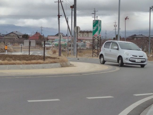
Sustainability 2020, 12, 1533                                                                          2 of 21

analysis tools are used to seek independent variables that determine the value of capacity. In these
models, all identifiable and measurable capacity determinants are usually sought. The form of the
function describing the capacity of a roundabout subordinate entry is then recorded in the following
general way:
                                  Cwl = f (G, S, D, W, T, L, M, E, O),                            (1)

where:

Cwl —roundabout entry capacity,
G—a set of geometrical features of a roundabout (e.g., external diameter, width of entries, width of
exits, width of the circulatory roadway),
S—a set of characteristics of traffic streams at the intersection (including vehicle traffic volumes at
entries, on the circulatory roadway of the intersection in collision areas, pedestrian traffic volumes in
the area of the intersection, cyclist traffic volume, traffic directional structure, traffic type structure),
D—a set of characteristics of drivers of vehicles involved in road traffic (e.g., gender, age, personality
traits, the motivation of driving, level of fatigue),
W—a set of characteristics describing weather conditions,
T—a set of temporal characteristics (e.g., year, month, day of the week, time, season),
L—a set of characteristics of the location of the intersection (e.g., land development area, outside the
land development area, peripheries of the land development area),
M—a set of characteristics of the development of the intersection’s surroundings (e.g., strict city center,
residential districts, green areas, recreational areas, dense land development),
E—a set of characteristics of environmental restrictions (including the permissible levels of noise of
transportation origin, exhaust emission level),
O—other characteristics that are often difficult to identify unambiguously.

     In statistical models, the behavior of drivers is represented by a relationship between the way an
intersection functions and its characteristics, which are very often geometric. Unfortunately, some
of the statistically important parameters, e.g., geometric ones, are difficult to interpret. Models
designed based on empirical data have some disadvantages, e.g., the process of collecting data from
measurements should take place when the entry capacity is exhausted, but this is difficult to achieve
in practice. The reliability of the results depends on the way of representation and the sample size.
Therefore, in order to obtain a reliable model, it is necessary to collect a large amount of data with
many variants of each examined parameter. The group of statistical models includes models presented,
among others, in [9–16].
     In the third group of models, i.e., in the group of simulation models, in addition to the elements
mentioned in the description of the two above groups of models, the dynamic characteristics of
particular vehicles, composite geometric situations, and other factors affecting the processes of the
presence and acceptance of gaps in the main stream may be taken into account.
     The substantial foundations of the gap acceptance theory for the main stream were developed
mainly by W. Siegloch [8], Harders [17], and W. Grabe [18]. One should also mention many valuable
works by J.C. Tanner [19,20], N. G. Major and D.J. Buckley [21]. It is most often assumed in models
designed based on the gap acceptance theory for the main stream of vehicles that the distribution
of gaps in the main stream is exponential (due to its relative simplicity in use compared to complex
multi-parametric distributions). This approach has been applied worldwide in a number of models
and methods used to calculate roundabout capacity, e.g., in Germany by W. Brilon [22–24], W. Brilon,
N. Wu and L. Bondzio [10], W. Brilon and B. Stuwe [25,26], W. Brilon, R. Koenig and R. Troutbeck [27],
W. Brilon and M. Vandehey [28]. In Poland, in the studies of J. Chodur [29], it is also the basis of the
model on which the method of calculating roundabout capacity was developed [30].
     More precise representation of conditions in roundabout traffic streams is possible with the use of
models in which the distribution of gaps between vehicles is described using distributions showing
Sustainability 2020, 12, 1533 3 of 21
the dependent traffic of vehicles. These models are modifications of the model developed by J.C.
Tanner, e.g., models based on the Cowan M3 distribution. J.C. Tanner was the first in 1962 to use the
Cowan M3 distribution to describe the time gaps in the traffic flow, and it was only in later years that it
began to be used to model the headways between moving vehicles. Its generalized form was used to
describe traffic conditions on roundabouts e.g., in Australia by R. J. Troutbeck [31] and R. Akçelik [32],
in Sweden by O. Hagring [33], or in Poland by E. Macioszek [34–37].
Although out of the three groups of models described above, models based on the gap acceptance
theory for vehicles at entries are considered to be the most reliable (due to the fact that they are models
that physically reflect given traffic phenomena), the latest research results, such as [11,12,38], indicate
the high accuracy of statistical models in the assessment of roundabout entry capacity. Such models
include the models contained in the HCM 2010 (Highway Capacity Manual) method [11] and in the
HCM 6th Edition method [12]. The construction of such models required considerable financial outlays
to perform numerous empirical studies under conditions of saturation of entries with traffic streams.
It is generally accepted that statistical models are not suitable for use in countries other than those for
which they were originally developed. The paper presents the effects of the analysis of the applicability
of the author’s model of the calculation of single-lane roundabout entry capacity (referred to as the E.
Macioszek model) developed for the conditions prevailing in Poland to the conditions prevailing at
single-lane roundabouts located in Tokyo and in Tokyo surroundings. The present research has been
financed from the funds of the Polish National Agency for Academic Exchange as part of the project
within the scope of the Bekker Programme. The project has the title “Analysis of the applicability of the
author’s method of roundabouts entry capacity calculation developed for the conditions prevailing in
Poland to the conditions prevailing at roundabouts in Tokyo (Japan) and in the Tokyo surroundings”.
2. The E. Macioszek Model
The E. Macioszek model was designed based on empirical data obtained from measurements
taken at roundabouts in Poland in 2004–2013. The model is constructed to calculate the value of
initial capacity of single-lane roundabouts, two-lane roundabouts, and turbo roundabouts under
the ideal conditions at the roundabout, i.e., without the influence of pedestrians and heavy traffic.
The value of actual capacity of roundabout entry can then be calculated using data about pedestrians
and heavy traffic volumes. This model is based on the gap acceptance theory with an empirical basis.
A detailed description of the model as well as detailed data about the model parameters can be found
in [39]. In the modeling process, a stepwise function of gap acceptance by vehicle drivers entering the
roundabout circulatory roadway is assumed. The model uses two different circulating stream headway
distributions according to the range of the circulating flow rate (Qnwl ). There are:
• for Qnwl ≤ 100 Pcu/h—shifted exponential distribution, and
• for Qnwl > 100 Pcu/h—Cowan M3 distribution.
The model used to calculate the initial capacity of a single-lane roundabout entry has the
following form:
Qnwl
−[ ·(t −t )]
3600−Qnwl ·tp g p
1.03·Qnwl ·e
h i
Pcu
f or Qnwl ≤ 100
Qnwl h
−[ ·t f ]
1−e 3600−Qnwl ·tp
Cowl = , (2)
φ·Qnwl
−[ ·(t g −tp )]
·φ·e 3600−Qnwl ·tp
1.03·Qnwl
h i h i
Pcu
f or Qnwl > 100 Pcu
φ·Qnwl h h
−[ ·t ]
3600−Qnwl ·tp f
1−e
where:
Cowl —the initial capacity for single-lane roundabout entry [Pcu/h],
Qnwl —the traffic volume on roundabout circulatory roadway [Pcu/h],
tg —critical gap [s],Sustainability 2020, 12, 1533 4 of 21
tf —follow-up time [s],
tp —minimum headway between vehicles moving on roundabout circulatory roadway [s],
φ—the proportion of unbunched vehicles for the circulating stream (φ ∈ h0, 1i)[–].
The summary or research data from single-lane roundabouts in Poland used for calibrating the
capacity model is presented in Table 1.
Table 1. The brief of research data from single-lane roundabouts used for calibrating the capacity model.
Parameter Single-Lane Roundabout
External diameter [m] 26.0–45.0
Central island diameter [m] 15.0–26.0
Circulating road width [m] 4.0–10.0
Total entry width [m] 3.0–4.0
Entry radius [m] 6.0–15.0
Total exit width [m] 4.0–4.75
Exit radius [m] 12.0–15.0
Number of intersection arms 4
Existence of splitter island Yes, at all entries
— —
Critical gaps [s] 3.16–6.05
Follow-up times [s] 2.50–3.08
Follow-up headway/critical gap ratio [–] 0.51–0.79
Traffic volume on circulatory roadway [Veh/h] 120–690
Sustainability 2020, 12, 1533 5 of 23
Total traffic volume on roundabout entry [Veh/h] 186–794
Figure 1 shows the initial capacity of single-lane roundabout entry calculated from the
E. Macioszek
Figure 1 showsmodel ascapacity
the initial a function of traffic
of single-lane volume entry
roundabout on the roundabout
calculated from thecirculatory
E. Macioszek
model as a function
roadway. of traffic
The curves arevolume on thefor
presented roundabout circulatory
extreme values roadway. data
of observed The curves areexternal
for the presented
for diameter
extreme values of observed data for the external
(Di) and circulatory roadway width (wc). diameter (D i ) and circulatory roadway width (wc ).
1. The1.initial
FigureFigure capacity
The initial of single-lane
capacity roundabout
of single-lane entry
roundabout calculated
entry from
calculated thethe
from E. E.
Macioszek model.
Macioszek
model.
3. Roundabouts in Japan
3.Although
Roundabouts in Japan are popular and often designed in many countries in Europe, North
roundabouts
America, Australia,roundabouts
Although and New Zealand, they are
are popular notoften
and a popular kind of
designed in intersections
many countriesin Japan. The vast
in Europe,
majority
NorthofAmerica,
intersections in Japan
Australia, and are controlled
New by they
Zealand, trafficare
lights.
not aThe first roundabout
popular in Japan was
kind of intersections
built
ininJapan.
2012 (by
Thecomparison, the first
vast majority roundabout in
of intersections inthe USAare
Japan wascontrolled
designed in by1905 in New
traffic York
lights. City,
The
whereas the first roundabout
first roundabout in JapaninwasEurope
builtwas built (by
in 2012 in 1905 in Paris. Both
comparison, theseroundabout
the first roundaboutsinarethestill
under operation). Some of the first roundabouts built in Japan included:
USA was designed in 1905 in New York City, whereas the first roundabout in Europe was
built in 1905 in Paris. Both these roundabouts are still under operation). Some of the first
roundabouts built in Japan included:
• 2012—Iida city and Karuizawa city in Nagano Prefecture—6 intersections were converted into
roundabouts,
• 2013—Yaizu city in Shizuoka Prefecture—2 intersections were converted into roundabouts,Sustainability 2020, 12, 1533 5 of 21
• 2012—Iida city and Karuizawa city in Nagano Prefecture—6 intersections were converted
into roundabouts,
• 2013—Yaizu city in Shizuoka Prefecture—2 intersections were converted into roundabouts,
• 2013—Moriyama city in Shiga Prefecture—2 intersections were converted into roundabouts.
Sustainability 2020, 12, 1533 6 of 23
According to data [40], 38 roundabouts were built in Japan in 2014, 49 in 2015, while according to
Japan Ministry of Land, Infrastructure, Transport, and Tourism [41], there are currently about 140 of
Prefecture
them in 32 Japanese prefectures (Figure 2). Roundabouts are primarily sited in residential areas as well
Osaka
as in suburban Miyagi
areas and further on in urban areas (Figure 3). There are only single-lane 6roundabouts.
Sustainability 2020, 12, 1533
Nara of 23
Kyoto
Hyogo
Prefecture
Fukuoka Osaka
Aichi
Miyagi
Kanagawa Nara
Nagano Kyoto
TokyoHyogo
Fukuoka
Saitama
TochigiAichi
Kanagawa
Kochi
Nagano
Prefecture
ShizuokaTokyo
Ishikawa
Saitama
Chiba
Tochigi
Hokkaido Kochi
Prefecture
Okinawa
Shizuoka
Ishikawa
Kagoshima
Hiroshima Chiba
Hokkaido
Okayama
Okinawa
Wakayama
Kagoshima
Gifu
Hiroshima
Ibaraki
Okayama
Aomori
Wakayama
Ehime Gifu
TokushimaIbaraki
Aomori
Yamaguchi
Ehime
Tottori
Tokushima
Mie
Yamaguchi
Niigata
Tottori
Mie
0
Niigata 2 4 6 8 10 12 14 16 18 20 22
0 2 4 6 Number
8 10of roundabouts
12 14 16 18 20 22
Number of roundabouts
Figure 2. Roundabouts in different prefectures in Japan. Source: own research based on [41].
2. Roundabouts
Figure Figure in different
2. Roundabouts prefectures
in different prefectures in Japan.Source:
in Japan. Source:
ownown research
research based based
on [41].on [41].
In front of the railway Other locations
station
In front of the railway Other6%
locations
1% station 6%
1%
Suburban area
Suburban area Residential areas
17%
17% Residential areas
64%
64%
Residential
Residential areasareas
Urban area
Urban area
Urban
Urban areaarea
12%12%
Suburban
Suburban area area
In front of the
In front ofrailway station
the railway station
Other locations
Other locations
(a)
(a)
Figure 3. Cont.Sustainability 2020, 12, 1533 7 of 23
Sustainability 2020, 12, 1533 6 of 21
Ellipse shape Less than 13 m
6% 1%
More then 46 m
12%
13 m or more and
less than 27 m
43%
Less than 13 m
27 m or more and 13 m or more and less than 27 m
less than 46 m 27 m or more and less than 46 m
38% More then 46 m
Ellipse shape
(b)
6 arms 8 arms
7% 1%
5 arms 3 arms
12% 21%
3 arms
4 arms
5 arms
6 arms
7 arms
4 arms
59%
8 arms
(c)
National road - city National road -
road province road - city
2% road
1%
Unknown
6%
Prefecture road- city
road
9%
City road - city road
82%
City road - city road
Prefecture road- city road
National road - city road
National road - province road - city road
Unknown
(d)
Figure
Figure 3. Selected
3. Selected roundabouts
roundabouts classification
classification in Japan,
in Japan, according
according to: (a)to: (a) location;
location; (b) external
(b) external diameter;
diameter; (c) the number of roundabout arms; (d) types of intersecting roads. Source:
(c) the number of roundabout arms; (d) types of intersecting roads. Source: Own research basedOwn research
on based on [41–45].
[41–45].
Although roundabouts have been operating within the transport network in Japan since 2012,
they are still not very popular and are not much liked by the Japanese. However, the reason for theirSustainability 2020, 12, 1533 7 of 21
use is the fact that they allow for smooth driving on intersections in crises such as earthquakes that
occur quite frequently in Japan, which is usually impossible during breakdowns at intersections with
traffic lights caused by earthquakes.
4. Roundabouts Entry Capacity Calculation—Case Study Based on Roundabouts in Tokyo and
Tokyo Surroundings
In order to analyze the applicability of the author’s model of roundabout entry capacity calculation
developed for the conditions prevailing in Poland to the conditions prevailing at roundabouts in
Tokyo and in Tokyo surroundings, examinations of traffic streams were performed for vehicles moving
around 6 single-lane roundabouts located in and around Tokyo using digital cameras from February to
April 2019. These were the following roundabouts:
• Minami Hanyu roundabout,
• Sakuragaocka roundabout,
• Suzaka Nagano roundabout
• Hitachi Taga roundabout,
• Iida Nagano 1 roundabout,
• Iida Nagano 2 roundabout.
Over the empirical measurements, the following features of traffic flows were identified:
• traffic volumes at roundabout entries at 15-min intervals,
• traffic volumes on the circulatory roadways of roundabouts at 15-min intervals,
• headways rejected and accepted by particular drivers at roundabout entries, which then were the
basis for determination of critical gaps (tg ),
• follow-up times (tf ) for drivers of vehicles from entries,
• headways between vehicles on the circulatory roadway (tp ),
• vehicle type structure,
• vehicle direction structure,
• empirical capacity.
The outer diameter of intersections (Di ) ranged from 24.0 to 37.0 m, whereas the roundabout
roadway (wc ) was between 4.0 and 5.0 m. The traffic was characterized by the volume ranging from
14 to 951 Pcu/h. There was between 0.1% and 10.0% of heavy vehicles recorded in the traffic stream.
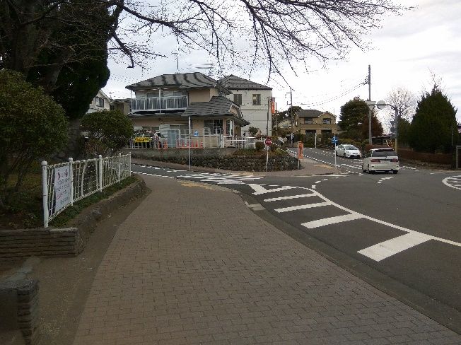
The measurements were performed under convenient weather conditions for traffic (no precipitation,
good visibility). In each case, the measuring stands were located in places as inconspicuous as possible
to the drivers (Figure 4). The number of samples for further analyses was selected from the Lapunov
formula with the level of significance set at 0.05.
The trajectories of the vehicles on the circulatory roadway and those at the entry were analyzed
using the Traffic Analyzer image processing system [46]. The position of vehicles was extracted in
0.5 s intervals, and then, the position coordinates were converted into a global coordinate system by
the projective transformation. The vehicle trajectories transformed were smoothened by the Kalman
smoothing method [47–49].
The analysis of the applicability of the E. Macioszek model of roundabouts entry capacity
calculation developed for the conditions prevailing in Poland to the conditions prevailing at roundabouts
in Tokyo and in the Tokyo surroundings consisted in determining the forms of functions representing
the parameters of the E. Macioszek model. These were functions that characterized:
• critical gaps (tg ),
• follow-up times (tf ) for drivers of vehicles from entries,
• minimum gaps between vehicles moving on roundabout circulatory roadways (tp ).Sustainability 2020,
Sustainability 12,12,
2020, 1533
1533 9 of 823of 21
measuring stations
measuring stations
(a) (b)
Figure4.4.Examples
Figure Examples of
of the locationof
the location ofmeasuring
measuringstations.
stations.
Due
Theto the fact that the
trajectories E. Macioszek
of the vehicles on model is based on the
the circulatory gap acceptance
roadway and those theory
at theand the function
entry were
of stepwise
analyzedacceptance
using theof the headways,
Traffic Analyzeritimage
was also necessarysystem
processing to conduct analyses
[46]. in orderoftovehicles
The position determine
thewas
formextracted
of the function
in 0.5 of the distribution
s intervals, of headways
and then, the position between vehicles were
coordinates moving on the circulatory
converted into a
roadway
global coordinate system by the projective transformation. The vehiclethe
of a roundabout. The data obtained in this way allowed for the calibration of E. Macioszek
trajectories
model to the conditions prevailing at roundabouts in Tokyo and in the Tokyo surroundings and then
transformed were smoothened by the Kalman smoothing method [47–49].
for the verification of the model using the measured empirical capacity.
The analysis of the applicability of the E. Macioszek model of roundabouts entry
4.1.capacity
The Choicecalculation developed
of the Distribution for theBetween
of Headways conditions Vehiclesprevailing in Poland
on the Circulatory to theofconditions
Roadway a Roundabout
prevailing at roundabouts in Tokyo and in the Tokyo surroundings consisted in
The main objective
determining the forms of theofanalysis in this
functions research areathe
representing wasparameters
to assess theofusefulness of theoretical
the E. Macioszek
models of a random variable to describe the headways between vehicles on the circulatory roadways
model. These were functions that characterized:
of roundabouts. The following theoretical distributions were used for the statistical analysis consisting
• verification
in the critical gaps of(tg),the zero hypothesis (H ) of the compatibility of the empirical distribution of
0
• follow-up times
headways with the hypothetical (tf) for drivers of vehicles of
distribution from theentries,
known form of F(t) distribution: exponential
• minimum gaps between vehicles moving on roundabout circulatory roadways (tp).
distribution, Erlang distribution, gamma distribution, log-normal distribution, exponential shifted
distribution,
Due to Cowan M3that
the fact distribution.
the E. Macioszek model is based on the gap acceptance theory and
the function of stepwisemodel
Tests of compatibility of distributions
acceptance of the with the real it
headways, distributions were performed
was also necessary with the
to conduct
χ Pearson’s
2
analyses in test,order
assuming the significance
to determine levelofα =
the form the0.05. The analyses
function of thewere carried out
distribution of independently
headways
forbetween
20 classesvehicles
of trafficmoving
volumeson with the span of 50 PCU/h. The test statistics were
the circulatory roadway of a roundabout. The data obtained in the form:
in this way allowed for the calibration of the E. Macioszek
2
model to the conditions
k n − n t
prevailing at roundabouts in Tokyo2 and in the Tokyo X i i surroundings and then for the
χemp = , (3)
verification of the model using the measured
i=1 i
nt
empirical capacity.
4.1. The Choice of the Distribution of Headways Between Vehicles
Xk on the Circulatory Roadway of a
Roundabout t t
ni = Npi , N = ni , (4)
i=1
The main objective of the analysis in this research area was to assess the usefulness of
t
p
theoretical models of a random i = P X adopted
variable
F the value
to describe class i , between vehicles on the (5)
theofheadways
circulatory roadways of roundabouts. The following
Critical value χ2 (α; k − u theoretical
− 1), distributions were used (6)
for the statistical analysis consisting in the verification of the zero hypothesis (H0) of the
where:
compatibility of the empirical distribution of headways with the hypothetical distribution
of the
k—the known
number form of F(t) distribution: exponential distribution, Erlang distribution,
of classes,
gamma distribution,
ni —class size, log-normal distribution, exponential shifted distribution, Cowan M3
distribution.
u—the number of unknown parameters of the hypothetical distribution F,
nti = Npti —theoretical (hypothetical) numbers,
α—the significance level.Sustainability 2020, 12, 1533 9 of 21
If χ2emp > χ2 (α; k − u − 1), the H0 hypothesis of the compatibility of empirical distribution with
theoretical distribution was rejected. The calculations were performed using the Statgraphics software.
They were performed independently for two states of the vehicle type structure, i.e., with and without
heavy vehicles, including passenger car units.
The conversion factor for heavy vehicles was used to determine the traffic volumes in passenger
car units per hour [Pcu/h]. It was determined based on the author’s own research as follows:
dtpc−hv
E= , (7)
dtpc−pc
where:
E —the conversion factor for heavy vehicles [–],
dtpc−hv —average gap between passenger car and heavy vehicle on the roundabout circulatory roadway
[s],
dtpc−pc —average gap between two passenger cars on the roundabout circulatory roadway [s].
The value of conversion factor for heavy vehicles (trucks and buses) to passenger car units
was obtained as E = 2.10. Table 2 contains the results of testing of the compatibility of individual,
accepted model distributions with the empirical distributions at the significance level α = 0.05 for
individual ranges of traffic volume. A positive result (marked with “+” in Table 2) was found to
be the one for which there were no grounds to reject the H0 hypothesis about the compatibility of
the empirical distribution with the selected hypothetical distribution for all the intersections tested.
Furthermore, a negative result (marked with “-” in Table 2) was considered to be a result for which at
least one of the intersections tested had grounds to reject the zero hypothesis. Given that there are
no grounds for rejecting the H0 hypothesis, there is no reason to question the compatibility of the
spacing distribution between vehicles on the circulatory roadway of a roundabout with the adopted
hypothetical distribution. The test is designed in such a way that as the value of the statistic χ2 gets
closer to zero, the H0 hypothesis becomes more reliable.
The analyses revealed that for small values of traffic volume (0–200 Pcu/h), the theoretical
distributions in most of the examined cases met the statistical conditions with the sufficient accuracy.
It was also found that in many cases, the distributions such as: exponential, shifted exponential,
log-normal, and gamma distribution can also describe the average traffic volume of vehicles passing
through a given road section (~200–400 Pcu/h). This is consistent with the results of the studies
published by C. Bennett [50], S. Yin et al. [51], E. Chevallier and L. Leclercq [52], or R. Rupali and P.
Saha [53]. However, from a traffic volume of approximately 400 Pcu/h, vehicle traffic is mainly not
smooth and these distributions (except for Cowan M3 and shifted exponential distribution) do not
meet the test condition χ2 . According to the literature [54,55], in situations of high traffic volume,
the distribution of headways between the vehicles on the circulatory roadways is mostly described by
exponential shifted distribution or complex distributions, such as the Hyperlang distribution, which is
a weighted sum of the shifted exponential and the Erlang distributions or the Cowan M3 distribution.
The aggregate results of the statistical tests presented in Table 2 prove that the most useful
theoretical distribution to describe the time headways between vehicles on the circulatory roadway of
a roundabout is the exponential shifted distribution. This is because it yields correct results for the
entire range of traffic volumes and for all roundabouts. Positive test results for all roundabouts and
traffic volumes greater than 250 Pcu/h were also obtained for the Cowan M3 distribution. Figure 5
presents a comparison of the accuracy of the description of empirical headway distributions for the
distributions tested. The quotient of the mean value χ2 calculated from the study and the critical value
was used to assess accuracy. As the value of this quotient gets closer to zero, the description becomes
more accurate. Furthermore, a value above 1.0 indicates a negative result of the compatibility of the
empirical distribution with the model distribution.Sustainability 2020, 12, 1533 10 of 21
Table 2. The outcome of the accuracy analysis of fit for the empirical and theoretical distributions
on a significance level α = 0.05 (where: “+” lack of reasons for rejecting the null hypothesis H0
about compliance of the empirical distribution with the theoretical distribution for all investigated
roundabouts, “-” there are reasons for rejecting the null hypothesis H0 for at least one test roundabout).
Theoretical Distribution Type
Traffic Volume
Range [Pcu/h] Shifted
Exponential Gamma Erlang Lognormal Cowan M3
Exponential
0–50 + + + + + -
50–100 + + + + + -
100–150 + + + - + -
150–200 + + + - + -
200–250 - + - - + -
250–300 + + - + + +
300–350 + + - + + +
350–400 + + - - + +
400–450 + - - - + +
450–500 - - - - + +
500–550 - - - - + +
550–600 - - - - + +
600–650 - - - - + +
650–700
Sustainability 2020, 12, 1533 - - - - + + of 23
12
700–750 - - - - + +
750–800 - - 2 - - + +
tested. The quotient of -the mean value
800–850 -
χ -calculated from
-
the study
+
and the critical
+
value850–900
was used to assess - accuracy. -As the value
- of this quotient
- gets+closer to zero,
+ the
900–950 becomes more
description - accurate.- Furthermore,
- +
a value- above 1.0 indicates +
a negative
950–1000 - - - - + +
result of the compatibility of the empirical distribution with the model distribution.
Figure 5. 5.Relative
Figure Relativevalues of χχ
values of 2 2statistic for theoretical distribution gaps between vehicles on the
statistic for theoretical distribution gaps between vehicles on the
roundabout circulatory roadway.
roundabout circulatory roadway.
TheThe
results of the
results of theanalyses contained
analyses in Figure
contained 4 confirm
in Figure veryvery
4 confirm highhigh
usefulness of the
usefulness ofshifted
the
exponential distribution
shifted exponential for describing
distribution the
for time headways
describing the between
time vehicles.
headways It should
between be emphasized
vehicles. It
χ2
that the quotient 2 obtained for this distribution
χ 2 in all tested ranges of traffic volume is very low,
χcritical
should
which be emphasized
proves the high accuracy that the
of quotient
the description of obtained for this distribution
actual headways. in all
Similar results in tested
terms of
χ critical
2
accuracy of the description of the analyzed distribution are obtained only for traffic volumes of above
ranges of traffic volume is very low, which proves the high accuracy of the description of
250 Pcu/h when Cowan M3 distribution is used.
actual headways. Similar results in terms of accuracy of the description of the analyzed
distribution are obtained only for traffic volumes of above 250 Pcu/h when Cowan M3
distribution is used.
4.2. The Minimal Headways between Vehicles on the Circulatory Roadway of a Roundabout
One of the very important parameters of the distribution of headways between
vehicles on the circulatory roadway of a roundabout is the minimum headway tp. TheSustainability 2020, 12, 1533 11 of 21
Sustainability 2020, 12, 1533 13 of 23
4.2.roadway
The Minimal Headways
which results between
fromVehicles on the Circulatory
a significant increase Roadway of a Roundabout
in the likelihood of vehicles rear
impacts. In cases
One of the of high traffic
very important volumes,
parameters of vehicles are moving
the distribution in columns
of headways betweenone vehicle
vehiclesafter
on the
another,roadway
circulatory and the of headways
a roundabout betweenis thevehicles
minimum are constants
headway tp . or
Thethey are similar
minimum headwayvalues to
between
each other.
vehicles on the So, in these
roadway of aroad traffic conditions,
roundabout minimumrole
plays an important values of tp headway
in calculating should of
the capacity bethe
subordinate entries of roundabouts.
sought. Considering the resultsAccording
of our own to the literature
research, [33], the
it was minimum
calculated thatobserved value of
the average
thevalue
distance
of tbetween
p headway vehicles
is equal ranges
to 2.45 from 0.5non-free
s (for to 2.5 s. Gaps
trafficshorter
conditions).than 1.0 s occur at intersections
or multi-lane
For theroads and are
collected observed
samples, the between
relationship vehicles travelling
between in different
the minimum lanes. According
headway tp and the to
R. Akçelik and E. Chung [54] or V. Statens [56], for roundabouts
traffic volume on the circulatory roadway of the roundabout Qnwl was analyzed. with one lane on the roundabout
Two
roadway, the minimum headway
different forms of the relationship t p ranges from 1.5 to 2.0 s and often is 1.8
were studied, but the power function was better suited s. Furthermore, some
studies, e.g., [55],
to empirical specify
data. Thethat the minimum
following form was values of tp headway greater than 2.0 s for roundabouts
obtained:
are rare.
t = 27.47 ⋅ Qnwl the[sauthor’s ] for own
−0.36
Considering the valuesp obtained from Qnwl > 100
tests, Pcube/ hstated
it can , (8)
that the minimum
headway
where:ranges from 2.31 to 5.74 s and clearly depends on the traffic volume. On the basis of data
presented on Figure 6, it can be concluded that stabilization of the minimum values of tp headway
tp—minimum
exists headway
for higher traffic volume between vehicles moving
on roundabout circulatoryon roadway
the roundabout circulatory
which results from aroadway
significant
[s],
increase in the likelihood of vehicles rear impacts. In cases of high traffic volumes, vehicles are moving
Qnwl—theone
in columns circulating flowanother,
vehicle after rate (i.e.,andtraffic volume onbetween
the headways the roundabout
vehicles arecirculatory
constants roadway)
or they are
[Pcu/h].
similar values to each other. So, in these road traffic conditions, minimum values of tp headway should
be sought.
TheConsidering
graphical formthe results
of theof our
above ownfunction
research,and it wasthecalculated
obtainedthat the average
empirical value
values of tp
are
headway is equal
presented to 2.456.s (for non-free traffic conditions).
in Figure
Figure
Figure 6. The
6. The dependence
dependence of of
thethe minimum
minimum headway
headway between
between vehiclesonon
vehicles the
the circulatoryroadway
circulatory roadwayas a
as a function
function of the traffic
of the traffic volume volume
on theon the roundabout
roundabout circulatory
circulatory roadway.
roadway.
ForBased on the analysis
the collected samples,oftheestimation accuracy
relationship between(Table
the 3), it was found
minimum thattpthe
headway assumed
and the traffic
power
volume on relationship
the circulatoryfor logarithmic
roadway values is well
of the roundabout Qnwl fit
was(aanalyzed.
relativelyTwo
small value
different of the
forms of the
coefficient of residual variation (Ve) of 13% and coefficient of convergence ( ϕ ) of 23%).
relationship were studied, but the power function was better suited to empirical data. 2The following
form was obtained:
Therefore, it can be assumed that the possible deviation of the actual headways between
the vehicles moving ontpthe = 27.47 · Qnwl −0.36
circulatory roadway ofnwla >
[s] for Q 100 Pcu/h, from the values of the (8)
roundabout
headways determined based on power function is relatively small. Furthermore, the
where:
analysis yielded a satisfactory value of the coefficient of determination (0.77) and the
tp —minimum
non-linear headway between
correlation vehicles
coefficient moving
(0.88), on confirms
which the roundabout circulatory
the existence roadway
of the [s],
relationship
Qnwl —the circulating
between flowunder
the variables rate (i.e., traffic volume on the roundabout circulatory roadway) [Pcu/h].
consideration.
The graphical form of the above function and the obtained empirical values are presented in
Figure 6.
Based on the analysis of estimation accuracy (Table 3), it was found that the assumed power
relationship for logarithmic values is well fit (a relatively small value of the coefficient of residual
variation (V e ) of 13% and coefficient of convergence (ϕ2 ) of 23%). Therefore, it can be assumed that theSustainability 2020, 12, 1533 12 of 21
possible deviation of the actual headways between the vehicles moving on the circulatory roadway of
a roundabout from the values of the headways determined based on power function is relatively small.
Furthermore, the analysis yielded a satisfactory value of the coefficient of determination (0.77) and the
non-linear correlation coefficient (0.88), which confirms the existence of the relationship between the
variables under consideration.
Table 3. The evaluation parameters of the estimated power function.
Parameter Parameter Value
Standard deviation of the residual component (Se ) 0.12
Coefficient of the residual variation (V e ) 0.13
Convergence factor (ϕ2 ) 0.23
Nonlinear correlation coefficient (R) 0.88
Determination coefficient (R2 ) 0.77
As the traffic volume on the circulatory roadway of a roundabout increases, the value of the
minimum headway between vehicles decreases. Apart from the traffic volume, the tp values may
be affected by other factors not taken into account in the analysis, such as local determinants of
geometric solutions, vehicle type structure, size of the city in which the roundabout was located,
weather conditions, etc.
4.3. Critical Gaps and Follow-Up Times Parameters for Vehicle Drivers at Roundabouts
M. Raff defined the critical gap as a value of time interval for which the number of accepted gaps
shorter than this value is equal to the number of rejected gaps longer than this value [57]. M. Raff and W.
Hart are authors of one of the first method of critical gap estimating. According to M. Raff, the critical
gap corresponds to the median (i.e., second quartile—50%) In the similar way, the critical gap value was
later determined D. Drew [58]. Critical gaps could be also calculated using the maximum likelihood
method [27]. In the estimation procedure of the maximum likelihood method, the probability of an
event that critical gap value is located between logarithm values: the largest rejected gap and gap
accepted by the individual drivers is determined. This method assumes that the sample obtained from
the measurements is the implementation of the event with the highest possible probability, which is
equivalent to the condition that credibility reaches a maximum.
The values of critical gaps were calculated using the cumulative distribution functions of the
accepted and rejected gaps as well as using the gap acceptance curves. The gap acceptance curves
were also used to calculate the critical gap as the gap for which the probability of acceptance is 50%.
The gaps were only collected for the vehicles on roundabout entry without any other vehicles ahead of
the entry give way line. An example of how the critical gaps were determined for the entry of the
Minami Hanyu roundabout using cumulative curves and the acceptance curve is presented in Figure 7.
The cumulative curves were calculated using the S. Raff method [57]. The values of critical gaps were
also calculated according to D. Drew dependency [58]:
(t3 − t1 )∆t
tg = t + [s] , (9)
(t2 + t3 ) − (t1 + t4 )
where:
t1 , t2 , t3 , t4 —the value of gaps that are sought in the sample in such a way as to meet the condition that
the number of accepted gaps (t1 , t2 ) smaller than the specified value t is similar (in the ideal case equal)
to the number of rejected gaps (t3 , t4 ) larger than the specified value t [s],
t—time value corresponding to the beginning of the interval in which the values were
located: t1 , t2 , t3 , t4 [s],
∆t—time interval [s].Sustainability 2020, 12, 1533 15 of 23
Δt—time interval [s].
The average value of the critical gap was equal to 4.69 s.
Sustainability 2020, 12, 1533 13 of 21
Number of gaps 2000 Accepted gaps
100
1800 Rejected gaps
90
1600 80
Percent of acceptance
of time intervals [%]
1400 70
1200 60
50
1000
40
800 30
600 20
400 10
0
200
0 1 2 3 4 5 6 7 8 9 10 11 12 13 14 15 16
0
0 1 2 3 4 5 6 7 8 9 10 11 12 13 14 15 16 Gaps [s]
Gaps [s]
(a) Minami Hanyu roundabout—entry 1.
2000
Number of gaps
Accepted gaps
1800 100
Rejected gaps 90
1600
Percent of acceptance
of time intervals [%]
80
1400
70
1200
60
1000 50
800 40
600 30
400 20
10
200
0
0
0 1 2 3 4 5 6 7 8 9 10 11 12 13 14 15 16
0 1 2 3 4 5 6 7 8 9 10 11 12 13 14 15 16
Gaps [s] Gaps [s]
(b) Minami Hanyu roundabout—entry 2.
2000
Accepted gaps
Number of gaps
1800 100
Rejected gaps
1600 90
Percent of acceptance
of time intervals [%]
80
1400
70
1200
60
1000 50
800 40
600 30
20
400
10
200 0
0 0 1 2 3 4 5 6 7 8 9 10 11 12 13 14 15 16
0 1 2 3 4 5 6 7 8 9 10 11 12 13 14 15 16
Gaps [s] Gaps [s]
(c) Minami Hanyu roundabout—entry 3.
2000 Accepted gaps
Number of gaps
1800 Rejected gaps 100
1600 90
Percent of acceptance
of time intervals [%]
80
1400
70
1200 60
1000 50
800 40
600 30
20
400
10
200 0
0 0 1 2 3 4 5 6 7 8 9 10 11 12 13 14 15 16
0 1 2 3 4 5 6 7 8 9 10 11 12 13 14 15 16
Gaps [s] Gaps [s]
(d) Minami Hanyu roundabout—entry 4.
Figure 7. The
Figure critical
7. The gap values
critical for thefor
gap values Minami HanyuHanyu
the Minami roundabout entry estimated
roundabout using (a)using
entry estimated cumulative
(a)
curves and (b)curves
cumulative acceptance curve.
and (b) acceptance curve.
The average value of the critical gap was equal to 4.69 s.
Next, the obtained data were subjected to regression and correlation analysis, which yielded
the dependence of the critical gap on the outer diameter of the roundabout (Di ) and width of the
circulatory roadway (wc ), and has the following form:
t g = 12.80 − 0.19 · Di − 0.56 · wc [s],
(10)
for 24 m ≤ Di ≤ 37 m, 4.0 m ≤ wc ≤ 5.0 m,Next, the obtained data were subjected to regression and correlation analysis, which
yielded the dependence of the critical gap on the outer diameter of the roundabout (Di)
and width of the circulatory roadway (wc), and has the following form:
t g = 12 .80 − 0.19 ⋅ Di − 0.56 ⋅ w c [ s ] ,
Sustainability 2020, 12, 1533 14 of 21
(10)
for 24 m ≤ Di ≤ 37 m , 4.0 m ≤ wc ≤ 5.0 m ,
where:
where:
tg—critical
tg —critical gapgap
[s], [s],
D i—external diameter
Di —external diameter of roundabout
of the the roundabout
[m], [m],
wc—width
wc —width of the
of the circulatory
circulatory roadway
roadway [m]. [m].
AA graphical
graphical representation
representation of linear
of the the linear multiple
multiple regression
regression function
function is shown
is shown in 8.
in Figure
Figure 8. The evaluation parameters of the estimated linear multiple function for the
The evaluation parameters of the estimated linear multiple function for the critical gap is presented in
critical
Table 4. gap is presented in Table 4.
Figure
Figure 8. 8.
TheThedependence
dependenceofofthe
the critical
critical gap
gap as
as aa function
functionofofthe
thecirculatory
circulatoryroadway width
roadway andand
width
roundabout
roundabout external
external diameter.
diameter.
Table 4. The
Table evaluation
4. The evaluationparameters
parametersof
ofthe
the estimated linearmultiple
estimated linear multiplefunction
functionforfor the
the critical
critical gap.
gap.
Parameter
Parameter Parameter Value
Parameter Value
Standard deviation of
Standard deviation of thetheresidual
residual component
component (Se(S
) e) 0.33
0.33
Coefficientofofthe
Coefficient theresidual
residual variation
variation (V(V
e ) e) 0.07
0.07
( ϕ) )
Convergence 2 2 0.19
Convergencefactorfactor(ϕ 0.19
Multiple correlation coefficient (R) 0.90
Multiple correlation coefficient (R) 0.90
Multiple determination coefficient (R2 ) 0.81
Multiple determination coefficient (R2) 0.81
It can be concluded
It can from
be concluded the the
from obtained correlation
obtained matrix
correlation (Table
matrix 4) that4)there
(Table is a linear
that there negative
is a linear
correlation between the variables t g and
negative correlation between the variables D i (the linear correlation coefficient for t g and
tg and Di (the linear correlation coefficient D is −0.88),
i for tg
and Di is −0.88), whereas the linear negative correlation between tg and wc is lower (linear tg
whereas the linear negative correlation between t g and w c is lower (linear correlation coefficient for
and wc is −0.60).
correlation coefficient for tg and wc is −0.60).
The multiple correlation coefficient (R) is 0.90, which indicates a very strong relationship of tg
The multiple correlation coefficient (R) is 0.90, which indicates a very strong
with Di and wc . The multiple determination factor (R2 = 0.81), indicates that 81% of the tg variability
relationship of tg with Di and wc. The multiple determination factor (R2 = 0.81), indicates
was explained by the variability of both Di and wc . The standard deviation of the residual component
that 81% of the tg variability was explained by the variability of both Di and wc. The
is 0.33, which indicates that the theoretical values of tg , determined from the estimated regression
standard deviation of the residual component is 0.33, which indicates that the theoretical
function, differ from the actual tg by ±0.33s. The coefficient of residual variability is 0.07. This means
values of tg, determined from the estimated regression function, differ from the actual tg by
that the standard deviation of the residual component accounts for 7% of the average tg value, which
±0.33s. The coefficient of residual variability is 0.07. This means that the standard deviation
in turn indicates moderate random variation. The coefficient of convergence is 0.19. Based on this
of the residual component accounts for 7% of the average tg value, which in turn indicates
measure of fit, it can be concluded that, in terms of the estimated multiple regression function, 19% of
the tg variability was not explained by the simultaneous change of the other two variables.
In addition to the explanatory variables adopted for the analysis (Di and wc ), many other variables
affect the critical gap simultaneously. Factors that may affect the critical gap values are also: traffic
factors (traffic volume for the main relation, distribution of gaps between vehicles of the main relation,
type of subordinate and closing vehicles, traffic volume of vehicles leaving the circulatory roadway
of a roundabout), and geometric factors (visibility restriction for subordinate vehicles, number of
roundabout entries, angle of intersection road axes, inclination of entries, separating islands at the
entries, etc.).gap values are also: traffic factors (traffic volume for the main relation, distribution of gaps
between vehicles of the main relation, type of subordinate and closing vehicles, traffic
volume of vehicles leaving the circulatory roadway of a roundabout), and geometric
factors (visibility restriction for subordinate vehicles, number of roundabout entries, angle
Sustainability 2020, 12, 1533
of intersection road axes, inclination of entries, separating islands at the entries, etc.). 15 of 21
Meanwhile, the follow-up times were estimated as an average value from follow-up
times of particular
Meanwhile, vehicletimes
the follow-up drivers
wereatestimated
each roundabout
as an average entry.
valueIndividual values
from follow-up of of
times
follow-up
particular timedrivers
vehicle were atanalyzed for the vehicles
each roundabout queuing at
entry. Individual the roundabout
values of follow-up entry,
time wereandanalyzed
then
the average value of follow-up time was established for the roundabout
for the vehicles queuing at the roundabout entry, and then the average value of follow-up time wasentry. The average
value of for
established follow-up time was
the roundabout equal
entry. toaverage
The 2.93 s (detailed analysis istime
value of follow-up presented in research
was equal work
to 2.93 s (detailed
[59]). is
analysis The obtained
presented in data were
research worksubjected
[59]). Theto regression
obtained data andwere
correlation
subjectedanalysis, whichand
to regression
yielded analysis,
correlation the dependence of the follow-up
which yielded time on
the dependence thefollow-up
of the outer diameter
time on ofthe
theouter
roundabout
diameter(D ofi)the
and width
roundabout (Dof
i ) the
and circulatory
width of theroadway (w
circulatory c ) and
roadway has the
(w c ) following
and has theform:
following form:
t f = 3.70 − 0.02 ⋅ Di − 0.06 ⋅ wc [ s ] ,
t f = 3.70 − 0.02 · Di − 0.06 · wc [s],for 24 m ≤ Di ≤ 37 m, 4.0 m ≤ wc ≤ 5.0 m, (11)(11)
for 24 m ≤ Di ≤ 37 m , 4.0 m ≤ wc ≤ 5.0 m ,
where:
where:
tf —- follow-up time [s],
tf—- follow-up time [s],
Di —- external
Di—- diameter
external diameterof the
of roundabout [m], [m],
the roundabout
wc —- width
wc—- of the
width circulatory
of the roadway
circulatory [m]. [m].
roadway
AA graphical
graphicalrepresentation of the
representation of linear multiple
the linear regression
multiple function
regression is shown
function in Figure
is shown in 9.
Furthermore, the evaluationthe
Figure 9. Furthermore, parameters of the
evaluation estimatedoflinear
parameters multiple function
the estimated for follow-up
linear multiple time is
function
presented in Table 5.
for follow-up time is presented in Table 5.
Figure
Figure 9. The
9. The dependenceofofthe
dependence thefollow-up
follow-up time
time as
as aa function
functionofofthe
thecirculatory
circulatoryroadway width
roadway andand
width
roundabout external diameter.
roundabout external diameter.
Table 5. The evaluation parameters of the estimated linear multiple function for follow-up time.
Parameter Parameter Value
Standard deviation of the residual component (Se ) 0.02
Coefficient of the residual variation (V e ) 0.01
Convergence factor (ϕ2 ) 0.02
Multiple correlation coefficient (R) 0.99
Multiple determination coefficient (R2 ) 0.98
It can be concluded from the obtained correlation matrix (Table 5) that there is a very strong linear
negative correlation between the variables tf and Di (linear correlation coefficient for tg and Di is −0.99)
and strong linear negative correlation between tf and wc (linear correlation coefficient for tf and wc
is −0.72). The linear positive correlation between the explanatory variables Di and wc is 80% (linear
correlation coefficient for Di and wc is 0.80).
The multiple correlation coefficient (R) is 0.99, which indicates a very strong relationship of tf
with Di and wc . The multiple determination factor (R2 = 0.98), indicates that as much as 98% of the tf
variation was explained by the variability of both Di and wc . The standard deviation of the residual
component is 0.02, which indicates that the theoretical values of tf , determined from the estimatedSustainability 2020, 12, 1533 16 of 21
regression function, differ from the actual tf only by ±0.02 s. The coefficient of residual variability is
0.01. This means that the standard deviation of the residual component accounts for 1% of the average
tf value, which in turn indicates very low random variation. The coefficient of convergence is 0.02.
Based on this measure of fit it can be concluded that, in terms of the estimated multiple regression
function, only 2% of the follow-up time variability was not explained by the simultaneous change of
the other two variables. With very small traffic volume on the circulatory roadway of the roundabout,
the follow-up times mainly determine the capacity of a given entry. Therefore, the relationship
describing the follow-up time should adequately reflect the actual conditions at the roundabout entry.
4.4. Implementation of the E. Macioszek Model to the Conditions Representing Driver Behaviour at
Roundabouts Located in Tokyo and Tokyo Surroundings
The E. Macioszek model presented in Section 2 was implemented to the conditions representing
driver behavior at roundabouts located in Tokyo and its surroundings. The implementation consisted
in using the model distribution of headways between vehicles on the circulatory roadway of a
roundabout obtained from empirical studies and analyses conducted at roundabouts in Tokyo and
Tokyo surroundings (Section 4.1), submodel representing the minimum headways between vehicles
moving on the circulatory roadway of a roundabout (Section 4.2), and submodels characterizing the
psychotechnical parameters i.e., critical gap and follow-up time representing the behavior of vehicle
drivers at roundabout entry (Section 4.3). The graphical form of the E. Macioszek model implemented
to the conditions representing the behavior of drivers at roundabouts in Tokyo and Tokyo surroundings
compared to 2020,
Sustainability the original
12, 1533 model is shown in Figure 10. 19 of 23
Figure 10. Implemented form of the E. Macioszek model to the conditions prevailing at roundabouts
Figure 10. Implemented form of the E. Macioszek model to the conditions prevailing at
in Tokyo and Tokyo surroundings.
roundabouts in Tokyo and Tokyo surroundings.
The correctness
The correctnessof the
of implemented
the implementedtraffictraffic
modelmodel
for single-lane roundabouts
for single-lane was verified
roundabouts was by
determination
verified by of the empiricalofcapacities
determination in the capacities
the empirical state of entry saturation
in the state of with
entrytraffic. Basedwith
saturation on the
obtained results, it can be concluded that on each of the analyzed single-lane roundabouts,
traffic. Based on the obtained results, it can be concluded that on each of the analyzed the relative
error values were
single-lane lower than 9.4%
roundabouts, (according
the relative errortovalues
[60], the model
were can than
lower be considered correct in
9.4% (according toterms
[60], of
accuracy
the model can be considered correct in terms of accuracy when the relative error values doalso
when the relative error values do not exceed 10.0%). Low absolute error values were
obtained, which
not exceed in all cases
10.0%). did not exceed
Low absolute 17 Pcu/h.
error values wereThe low
also values ofwhich
obtained, relative
in and absolute
all cases errors
did not
prove
exceed 17 Pcu/h. The low values of relative and absolute errors prove that the capacity of
that the capacity calculated by the proposed model is highly consistent with the actual capacity
single-lane
calculatedroundabout
by the entries.
proposedThismodel
demonstrates the adoption
is highly consistentof appropriate headway
with the actual distributions
capacity of
describing the flow of vehicles on the circulatory roadway of a single-lane roundabout,
single-lane roundabout entries. This demonstrates the adoption of appropriate headway and functions
describing the parameters of these distributions. An additional factor that ensured the most adequate
distributions describing the flow of vehicles on the circulatory roadway of a single-lane
representation of traffic in the area of single-lane roundabouts was the use of digital cameras in
roundabout, and functions describing the parameters of these distributions. An additional
measurements which guaranteed the appropriate accuracy of measurement of the tested characteristics.
factor that ensured the most adequate representation of traffic in the area of single-lane
roundabouts was the use of digital cameras in measurements which guaranteed the
appropriate accuracy of measurement of the tested characteristics. The results of the
analysis of model accuracy also indicate that all the average error values can be considered
as small, falling within the accuracy range of the currently used measurement methods.
5. DiscussionsYou can also read