Rough-Terrain Locomotion and Unilateral Contact Force Regulations With a Multi-Modal Legged Robot
←
→
Page content transcription
If your browser does not render page correctly, please read the page content below
Rough-Terrain Locomotion and Unilateral Contact Force Regulations
                                                          With a Multi-Modal Legged Robot
                                                            Kaier Liang, Eric Sihite, Pravin Dangol, Andrew Lessieur, and Alireza Ramezani1

                                                                                                                                                                   ut Thruster Forces
                                            Abstract— Despite many accomplishments by legged robot
                                         designers, state-of-the-art bipedal robots are prone to falling
                                         over, cannot negotiate extremely rough terrains and cannot                                                                 Thruster Actuator
                                         directly regulate unilateral contact forces. Our objective is to
                                         integrate merits of legged and aerial robots in a single platform.
arXiv:2103.15952v1 [cs.RO] 29 Mar 2021

                                         We will show that the thrusters in a bipedal legged robot called                                                                  Thruster
                                         Harpy can be leveraged to stabilize the robot’s frontal dynamics
                                         and permit jumping over large obstacles which is an unusual
                                                                                                                                                                         Hip Frontal
                                         capability not reported before. In addition, we will capitalize on
                                                                                                                                                                         Actuator
                                         the thrusters action in Harpy and will show that one can avoid
                                         using costly optimization-based schemes by directly regulating
                                         contact forces using an Reference Governor (RGs). We will                                                                       Hip Sagi al
                                         resolve gait parameters and re-plan them during gait cycles by                                                                  Actuator
                                         only assuming well-tuned supervisory controllers. Then, we will
                                         focus on RG-based fine-tuning of the joints desired trajectories                                                              Knee Actuator
                                         to satisfy unilateral contact force constraints.
                                                                                                                                                                   ug Ground Reaction
                                                                 I. I NTRODUCTION                                                                                            Force

                                            Raibert’s hopping robots [1] and Boston Dynamics’ robots
                                         [2] are amongst the most successful examples of legged
                                         robots, as they can hop or trot robustly even in the presence
                                         of significant unplanned disturbances. Other than these suc-
                                                                                                                    Fig. 1. Illustration of a concept design for Harpy, a thruster-assisted bipedal
                                         cessful examples, a large number of underactuated and fully                robot designed by the authors to study robust, efficient and agile legged
                                         actuated bipedal robots have also been introduced. Agility                 robotics.
                                         Robotics’ Cassie [3], Honda’s ASIMO [4] and Samsung’s
                                         Mahru III [5] are capable of walking, running, dancing and                 very limited in that, for example, the height of terrain bumps
                                         going up and down stairs, and the Yobotics-IHMC [6] biped                  should not exceed the size of the legs [7], [8], [9]. However,
                                         can recover from pushes. Despite these accomplishments,                    a legged robot maintains a superior energetic efficiency of
                                         all of these systems are prone to falling over and cannot                  locomotion because its overall body weight is supported by
                                         negotiate extremely rough terrains. Even humans, known                     the legs, can safely operate inside buildings and has no sharp,
                                         for their natural, dynamic and robust gaits cannot recover                 rotating blades to cause severe laceration injuries to humans.
                                         from severe rough terrain perturbations, external pushes                      Thruster-assisted legged locomotion has not been explored
                                         or slippage on icy surfaces. Our goal is to enhance the                    previously except to a limited extent in a few examples
                                         robustness of these systems through a distributed array of                 that only considered the hardware-related challenges [10].
                                         thrusters and nonlinear control.                                           These robots potentially can offer rich and challenging dy-
                                            In this paper, we will report our efforts in designing                  namics and control problems. The overactuation and control
                                         closed-loop feedback for the thruster-assisted walking of a                allocation problems led by the coexistence of thrusters and
                                         legged system called Harpy (shown in Fig. 1), currently its                joint actuators not only can provide opportunities to study
                                         hardware being developed at Northeastern University. This                  interesting control ideas, but also, from a dynamical behavior
                                         biped is equipped with a total of eight actuators, and a pair              standpoint, can permit studying unexplored behaviors such
                                         of coaxial thrusters fixed to its torso. Our motivation stems              as walking under buoyancy phenomena [11]. Also, studying
                                         from the merits of aerial and legged systems and we intend                 multi-modal systems that can switch from one mode to
                                         to integrate these merits in a single platform. Contrary to                another in order to overcome the demanding mobility objec-
                                         fixed- or rotary-wing aerial systems, legged robots cannot                 tives in unstructured environments is a rather new research
                                         exhibit a fast mobility and fly over obstacles. A legged                   problem and potentially can result in interesting machine-
                                         robot’s capability to negotiate extremely bumpy terrains (e.g.,            learning and optimization-based motion planning problems
                                         semi-collapsed buildings in the aftermath of an earthquake) is             [12].
                                            1 SiliconSynapse Laboratory, ECE Department, Northeastern Univer-
                                                                                                                       From a feedback design standpoint, the challenge of simul-
                                         sity, Boston, MA, USA. emails: {liang.k, e.sihite, dangol.p, lessieur.a,   taneously providing asymptotic stability and gait feasibility
                                         a.ramezani} @northeastern.edu                                              constraints satisfaction in legged systems have been exten-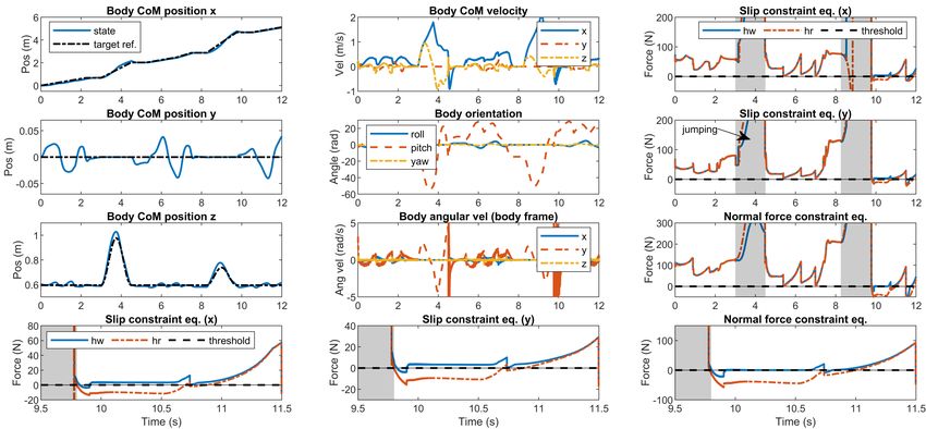
sively addressed [13]. For instance, the method of Hybrid
Zero Dynamics (HZD) has provided a rigorous model-based
approach to assign attributes such as efficiency of locomotion
in an off-line fashion. Other attempts entail optimization-
based, nonlinear approaches to secure safety and perfor-
mance of legged locomotion [14], [15], [16], [17], [18], [19].
   Thrusters can result in unparalleled capabilities. For in-
stance, gait trajectory planning (or re-planning), control and
unilateral contact force regulation can be treated significantly
differently as we have shown previously [20], [21], [22]
and will further discuss new details in this paper. That
said, real-time gait trajectory design in legged robots has
been widely studied and the application of optimization-
based methods is very common [23]. In general, in these
paradigms, an optimization-based controller adjusts the gait
parameters throughout the whole gait cycle such that not only
the robot’s posture is adjusted to accommodate the unplanned
posture adjustments but also the joints position, velocity and      Fig. 2. Shows the joint movements, key positions (pi ) and dimensions (li )
acceleration are modified to avoid slipping into infeasible         of Harpy. The non-conservative forces and torques acting on the system are
scenarios, e.g., the violation of contact forces. What makes        denoted by ui .
these methods further cumbersome is that they are widely
defined based on Whole Body Control (WBC) which can                    This paper is outlined as follows: the dynamic modeling
lead to computationally expensive algorithms [24].                  for Harpy and the reduced-order models which will be used
   These problems are widely known to suffer from curse of          in the numerical simulation and controller design, the discus-
dimensionality and other popular paradigms such as Approx-          sion on thruster assisted locomotion, numerical simulation
imate Dynamic Programming (ADP) [25], Reinforcement                 discussions, and then followed by the concluding remarks.
Learning (RL) [26], decoupled approaches to design control
for nonlinear stochastic systems [27], etc., can potentially                     II. DYNAMIC M ODELING OF H ARPY
remedy the challenges. However, these approaches are far               This section outlines the dynamics formulation of the robot
from providing any practical solutions to the problem in hand       which is used in the numerical simulation in Section IV, in
and they are shown to be only effective on simpler practical        addition to the reduced order models which are used in the
robots mainly those that can only demonstrate quasi-static          controller design. Fig. 2 shows the kinematic configuration
gaits.                                                              of Harpy which listed the center of mass (CoM) positions
   We will capitalize on the thrusters action in Harpy and          of the dynamic components, joint actuation torques, and
will show that one can limit the use of costly optimization-        thruster torques. The system model has a combined total of
based schemes by directly regulating contact forces. We             12 degrees-of-freedoms (DoFs): 6 for the body and 3 on each
will resolve gait parameters and re-plan them during the            leg. Due to the symmetry, the left and right side of the robot
whole Single Support (SS) phase, which is the longest phase         follow a similar derivations so only the general derivations
in a gait cycle, by only assuming well-tuned supervisory            are provided in this section.
controllers found in [28], [29], [30] and by focusing on
fine-tuning the joints desired trajectories to satisfy unilateral   A. Euler-Lagrange Formalism
contact force constraints. To do this, we will devise inter-           The Harpy equations of motion are derived using Euler-
mediary filters based on the celebrated idea of Explicit Ref-       Lagrangian dynamics formulation. In order to simplify the
erence Governors (ERG) [31], [32], [33], [34]. ERGs relied          system, each linkages are assumed to be massless and the
on provable Lyapunov stability properties can perform the           mass are concentrated at the body and the joint motors.
motion planning problem in the state space in a much faster         Consequently, the lower leg kinematic chain is considered to
way than widely used optimization-based methods. That said,         be massless which significantly simplifies the system. The
these ERG-based gait modifications and impact events (i.e.,         three leg joints are labeled as the hip frontal (pelvis P ), hip
impulsive effects) can lead to severe deviations from the           sagittal (hip H) and knee sagittal (knee K), as illustrated in
desired periodic orbits and standard legged robots cannot           Fig. 2. The thrusters are also considered to be massless and
sustain these perturbations. Previously, we demonstrated that       capable of providing forces in any directions to simplify the
the thrusters can be leveraged to enforce hybrid invariance in      problem.
a robust fashion by applying predictive schemes within the             Let γh be the frontal hip angle while φh and φk be the
Double Support (DS) phase [22]. Last, we also will show             sagittal hip and knee angles respectively. Let the superscript
that thrusters can be leveraged to stabilize frontal dynamics       {B, P, H, K} represent the frame of reference about the
and permit jumping over large obstacles which is an unusual         body, pelvis, hip, and knee while the inertial frame is repre-
capability not reported before.                                     sented without the superscript. Let RB be the rotation matrix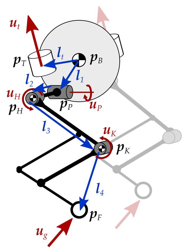
from the body frame to the inertial frame (i.e. x = RB xB ). ug is the ground reaction forces (GRFs). The variables M ,
The pelvis motor mass is added to the body mass. Then h, Bt , and Bg are a function of the full system states:
the positions of the hip and knee CoM are defined using >
x = [rB , q > , φKL , φKR , ωB
B>
, q̇ > , φ̇KL , φ̇KR ]> , (6)
kinematic equations:
where the vector rB contains the elements of RB . Using
pP = pB + RB l1B , pH = pP + RB Rx (γh ) l2P
(1) Bj = [06×6 , I6×6 ] allows uj to actuate the joint angles
pK = pH + RB Rx (γh ) Ry (φh )l3H , directly. Let v = [ωB B>
, q̇ > ]> be the velocity of the gen-
where Rx and Ry are the rotation matrices about the x and eralized coordinates, then Bt and Bg can be defined using
y axis respectively, l is the length vectors representing the the virtual displacement from the velocity as follows:
conformation of Harpy which are constant in their respective
> >
∂ ṗTL /∂v ∂ ṗFL /∂v
local frame of reference. The foot and thruster positions are Bt = ∂ ṗTR /∂v , Bg = ∂ ṗFR /∂v . (7)
defined as: 02×6 02×6
pF = pK + RB Rx (γh ) Ry (φh ) Ry (φk ) l4K
(2) The vector ut = [u> > >
tL , utR ] is formed from the left and
pT = pB + RB ltB thruster forces utL and utR , respectively.
The GRF is modeled using the unilateral compliant ground
where the length vector from the knee to the foot is l4K =
model with undamped rebound while the friction is modeled
[−l4a cos φk , 0, −(l4b + l4a sin φk )]> which is the kinematic
using the Stribeck friction model, defined as follows:
solution to the parallel linkage mechanism of the lower
leg. Let ωB be the angular velocity of the body. Then ug,z = − kg,p pF,z − kg,d ṗF,z
the angular velocities of the hip and knee are defined as: |ṗF,x |2
ωHB
= [γ̇h , 0, 0]> + ωB
B
and ωK H
= [0, φ̇h , 0]> + ωH H
. ug,x = − µc + (µs − µc ) exp − fz sgn(ṗF,x )
vs2
Finally, the energy of the system for the Lagrangian
− µv ṗF,x ,
dynamics formulation are defined as follows: (8)
1P
> i> ˆ i
where pF,x and pF,z are the x and z components of the
K= m i p i p i + ω i I i ω i inertial foot position, kg,p and kg,d are the spring and
2 Pi∈F (3)
> > damping model for the ground, µc , µs , and µv are the
V = − i∈F mi pi [0, 0, −g] ,
Coulomb, static, and viscous friction coefficient respectively,
where F = {B, HL , KL , HR , KR } are the relevant frame and vs is the Stribeck velocity. kg,d = 0 if ṗF,z > 0 for the
of references and mass components (body, hip and knee of undamped rebound model and the friction in the y direction
each side), and the subscripts L and R represent the left follows a similar derivation to ug,x . Then the ground force
and right side of the robot. Furthermore, Iˆi is the inertia model ug is defined as follows:
about its local frame, and g is the gravitational constant.
This forms the Lagrangian of the system L = K − V which ug = [u> > >
gL H(−pFL ,z ), ugR H(−pFR ,z )] , (9)
is used to derive the system’s Euler-Lagrangian equations of where H(x) is the heaviside function, while ugL and ugR
motion. The dynamics of the body angular velocity is derived are the left and right ground forces which are formed using
using the modified Lagrangian for rotation in SO(3) to avoid their respective ug,x , ug,y , and ug,z . Finally, the full system
using Euler angles and the potential gimbal lock associated equation of motion can be derived using (4) to (9) to form
with them. This results in the following equations of motion ẋ = f (x, uj , ut , ug ).
following Hamilton’s principle of least action:
B. Reduced-Order Models
d ∂L B ∂L P3 ∂L
B
+ ωB × B
+ j=1 rBj × = u1 The following reduced-order models are used: a variable
dt ∂ωB ∂ωB ∂rBj
length inverted pendulum (VLIP) model and a two-body
d ∂L ∂L d B pendulum model, as illustrated in Fig. 3. The VLIP model is
− = u2 , RB = RB [ωB ]× ,
dt ∂ q̇ ∂q dt used to describe walking with an ERG, while the two-body
(4) pendulum model is used to describe the flight phase with
>
where [ · ]× is the skew operator, RB = [rB1 , rB2 , rB3 ], a Model Predictive Control (MPC) to track trajectory and
q = [p> B , γhL , γhR , φhL , φhR ]
>
is the dynamical system regulate the appropriate leg postures at the time of landing.
B
states other than (RB , ωB ), and u is the generalized forces. 1) Variable-Length Inverted Pendulum (VLIP) Model:
The knee sagittal angle φk which is not associated with As shown in Fig. 3a, the model is described simply using
any mass is updated using the knee joint acceleration input the inverted pendulum model where the length of r can be
uk = [φ̈kL , φ̈kR ]> . Then the system acceleration can be adjusted through the change in leg conformation. The center
derived as follows: of pressure, c, is defined as the weighted average position of
M a + h = Bj uj + Bt ut + Bg ug (5) the foot, c = λL pFL + λR pFR , where λi = ugi ,z /(ugL ,z +
ugR ,z ), i ∈ {L, R}. Harpy is modeled using a point foot, so
where a = [ω̇BB>
, q̈ > , φ̈kL , φ̈kR ]> , ut is the thruster force, c is equal to the stance foot position during the SS phase.
uj = [uPL , uPR , uHL , uHR , u> >
k ] is the joint actuation, and The VLIP model without thrusters is underactuated, but the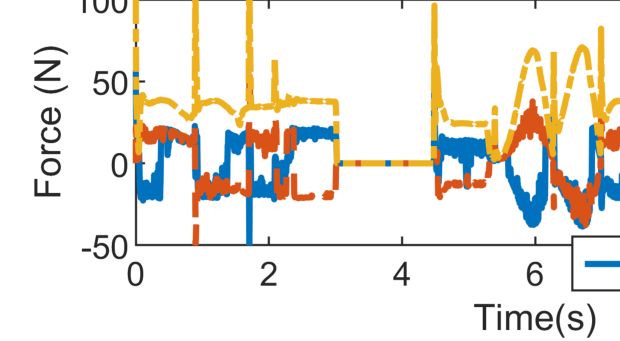
addition of thrusters makes the system fully actuated and
enables it to do trajectory tracking.                                                pB        Jsλ
  The dynamic model is derived as follows:
                                                                                                                pB

                 mp̈B = mg + ut,c + Js> λ                (10)                                   ut                   pH θ
                                                                               r
                                                                                          mg
where m is the mass of the pendulum which in this case is
the total mass of the system, and ut,c is the thruster forces                                                          q         pK
about the body CoM. The constraint force Js> λ is setup to
keep the leg length r equal to the leg conformation using the           c                                    m1 g
following constraint equation:                                                                                                  m2 g
                                                                               (a)                                     (b)
         Js (p̈B − c̈) = ur ,     Js = (pB − c)> ,       (11)
                                                                 Fig. 3. Illustrates two reduced-order models, a variable-length inverted
which is designed to keep the leg length second derivative       pendulum (VLIP) and a two-body pendulum model, which are used to
                                                                 describe the dominant dynamic response of the system during the walking
equal to ur . This constraint force also forms the GRF as        and ballistic motions, respectively.
long as the friction cone constraint is satisfied. Assuming no
slip (c̈ = 0), then the inputs to the system are ur which
controls the body position about the vector r = pB − c by        parameters P0 , P2 , and P4 define the initial, middle, and
adjusting the leg length, and the thrusters ut which controls    final positions of the gait. Each swing and stance feet-end
the remaining DoFs.                                              have a constant Bezier curve parameters to form the 2D
   2) Two-body Pendulum Model: As shown in Fig. 3b, the          open-loop walking gait. The following parameters defined
model is described as a planar double pendulum in the x-         in the x-z plane are used: P0,sw = [−0.21, −0.60]> m ,
z plane where the mass is concentrated in the body CoM           P2,sw = [−0.20, −0.50]> m, and P4,sw = [0.10, −0.60]> m
and knee, m1 and m2 respectively. Here, the mass of the          for the swing foot, and P0,st = [0.10, −0.60]> m , P2,st =
pelvis motors are combined into the m1 while the mass            [0.01, −0.63]> m, and P4,st = [−0.21, −0.60]> m for the
of both hips are combined into m2 to ensure a similar            stance foot. These Bezier parameters define the feet positions
kinematics behavior. The control action is defined as udp =      and then the joint angles are found simply by resolving
[ux , uz , uh ]> where ux and uz are the sum of thruster         the corresponding inverse kinematics problem. Finally, these
forces in the x and z directions, respectively, and uh is the    joint trajectories are tracked using an asymptotically stable
sagittal hip motor torque. The model uses the following states   controller [35].
qdp = [pB,x , pB,z , q, θ]> , where q is the hip joint angle        The thrusters are used to stabilize the roll and yaw motion
and θ is the body absolute pitch angle. Then the system          of the robot using the following controller
acceleration can be derived as follows:
                                                                     utL ,F = [uyaw , 0, uroll ]> ,       utR ,F = −utL ,F ,        (13)
                 Mdp q̈dp + hdp = Bdp udp ,              (12)
                                                                 where utL ,F and utR ,F are the left and right thruster force
where Bdp = [I3×3 , 01×3 ], allows the direct control signal     components for frontal dynamics stabilization, while uroll
to the system states except θ.                                   and uyaw are simple PD controllers to track zero roll and yaw
                                                                 reference angles. This controller is sufficient to stabilize the
 III. C ONTROL OF T HRUSTER -A SSISTED L OCOMOTION
                                                                 frontal dynamics and the robot’s heading even when using
   This section discusses and outlines the applications of       a gait designed for a 2D bipedal robot. During walking, the
thrusters in our robot, particularly to stabilizes the frontal   combined thruster forces are formed by combining ut,c in
dynamics, apply the ERG framework to regulate GRFs, and          (10) and (13), as follows
to perform ballistic motions to avoid obstacles.
                                                                             ut = [u>      > >          >        >      >
                                                                                    t,c , ut,c ] /2 + [utL ,F , utR ,F ] .          (14)
A. Frontal Dynamics Stabilization
   In order to show the application of thruster-assisted walk-   B. Thruster-Assisted Enforcement of GRF Constraints Using
ing in our robot, we use a walking gait designed for a planar    RG-based Methods
bipedal robot. The absence of the frontal dynamics means            The ERG framework is utilized to enforce the friction
that this gait is unstable for 3D walking. Hence the thrusters   pyramid constraint of the robot by manipulating the applied
are used to stabilize the robot’s roll and yaw to achieve a      reference to the controller, which is useful to avoid using
stable walking gait in the full 3D system.                       optimization or nonlinear MPC framework to enforce con-
   The gait is designed by constraining the system dynamics      straints on the harder-to-model GRFs. The VLIP model in
in the x-z plane using 4th order Bezier polynomials to           (10) can be fully actuated due to the addition of thrusters,
define the feet-end positions relative to the hip in the robot   which enables us to utilize a more advanced controller such
body frame (pB           B
                  F − pP ). Let Pi , i ∈ {0, . . . , 4} be the   as ERG.
Bezier polynomial parameters. This 4th order polynomial             The ERG manipulates the applied reference (xw ) to avoid
can be constrained to have zero initial and final gait ve-       violating the constraint equation hw (x, xw ) ≥ 0 while
locity by setting P0 = P1 and P3 = P4 . Then the free            also be as close as possible to the desired reference (xr ),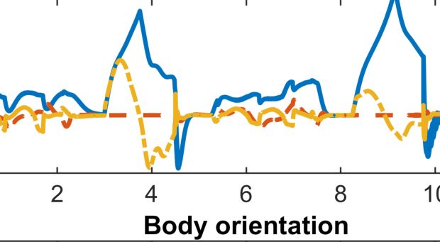
as illustrated in Fig. 4. Consider the Lyapunov equation hw < 0 V
V = (xr − xw )> P (xr − xw ). xw is updated through the hr < 0 min
update law:
ẋw = vr + vt + vn , (15)
vn xr
where vr drives xw directly to xr , while vt and vn drives xw vr V=0
along the surface and into the constraint equation boundary xw vt
hw = 0, respectively. The objective of this ERG algorithm is xw,t hw = 0
to drive xw to the state xw,t which is the minimum energy hw > 0
solution Vmin that satisfies the constraint hw ≥ 0.
Let hr (x, xr ) = Jr xr + dr ≥ 0 be the constraint Fig. 4. Shows how an Explicit Reference Governor (ERG) can manipulate
equation using the desired reference xr , and Cr be the the applied reference states xw to be as close as possible to the desired
reference xr while the constraint equations hw ≥ 0 remain feasible.
rowspace of the violated constraints of hr . Define Nr =
null(Cr ) = [n1 , . . . , nn ] where n is the size of the nullspace.
Additionally, let rk be the k’th row of Jr . Then the following is aligned about the body CoM sagittal axis. Therefore, the
update law is used for vr , vt , and vn : reduced-order model in (5) is used to model the robot during
the ballistic motion which is represented as a two-body
vr = α̂r (xr − xw ), vn = α̂n rk rk> (xr − xw )
Pn (16) pendulum system. Then an MPC framework is developed
vt = k=1 α̂t nk n>
k (xr − xw ), based on this model to regulate the feet-end positions and
where α̂ are scalars defined as follows: ensuring the proper landing configuration.
( The hip frontal and knee angles are setup to be constant
αr , if min(hw ) ≥ 0 or min(hr ) ≥ 0 during the ballistic maneuver and the feet are positioned in a
α̂r =
0, else neutral stance configuration within which legs are parallel to
( each other. An MPC with a prediction and control horizons
αt , if min(hw ) ≥ 0 or min(hr ) < 0
α̂t = Nh = 10 is developed using the following optimizer
0, else (17) PNh k>
min k=0 (e We ek + ∆uk> k
dp Wu ∆udp )∆t
αn ,
if min(hw ) ≤ min(hr ) < 0 udp
α̂n = −αn , if min(hr ) < min(hw ) < 0 subject to ẋdp = f (xdp , udp ) (19)
k+1 k
0, else, qref − θ + qc = 0
where α is a positive scalar which determines the rate of |udp | − udp,max ≤ 0,
convergence. where e = [p> > >
B −pB,ref , q −qref ] is the tracking error, We
Assuming ẋr = 0 and using the update law defined from and Wu are the cost weighting matrices, and qc is a constant
(16) and (17), we willP have V̇ = −2(xr −xw )> Q (xr −xw ), angle to determine the desired landing posture. qref denotes
n
with Q = P (α̂r I + k=1 α̂t nk n> >
k + α̂n rk rk ). We have the reference hip sagittal angle which is updated each time
the gradient V̇ = 0 if min(hw ) ≤ 0 and nk ⊥(xr − xw ), step relative to the body pitch angle θ and qc . This reference
while V̇ < 0 when min(hr ) ≥ 0 or when min(hw ) ≥ 0. In can ensure the legs do not lag behind the body at the landing
case both applied reference and target constraints equation moment, and qc can be properly adjusted to achieve the
are violated, we have V̇ > 0 which drives the xw towards the desired landing posture. The references pB,ref are designed
constraint boundary. This allows the xw to converge to xw,t as a ballistic motion for the body CoM as follows
which is the minimum energy solution that satisfies hw ≥ 0 >
as illustrated in Fig. 4. pk+1 k
B,ref = pB,ref + ∆t [a, b sin(2πt/1.5)] (20)
The GRF constraints for this robot can be derived from where pB denotes the body position in the x-z plane, while a
the reduced-order model constraint equation in (11) by ap- and b are some constants, and ∆t is the controller time step.
plying the ground pyramid constraint. We use the following Finally, the resulting udp = [ux , uz , uh ] is fed to the full
constraints for the ERG: model, where the thruster forces ux and uz are combined
|ug,x |≤ µs ug,z , |ug,y |≤ µs ug,z , ug,z ≥ uz,min , (18) with the roll and yaw stabilization controller in (13). This
forms the combined thruster forces
where [ug,x , ug,y , ug,z ]> = Js> λ is the ground reaction force
model from (10) and (11). This forms the ground friction ut = [ux , 0, uz , ux , 0, uz ]> /2 + [u> > >
t,l , ut,r ] , (21)
pyramid constraint and the minimum ground normal force which tracks the flight trajectory and stabilizes the robot’s
acting on the leg to ensure that the foot doesn’t slip. roll and heading angles.
C. MPC Design and Control of Robot’s Ballistic Motion IV. S IMULATION R ESULTS
The thrusters can also be used to traverse rough terrain by The optimization and numerical simulation are done in
simply flying over obstacles. However, it is not possible to Matlab where we used interior-point algorithm and RK4
stabilize pitch dynamics due to the thrusters position which scheme, respectively. The MPC and the ERG filter are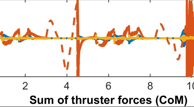
(a)
(b)
(c)
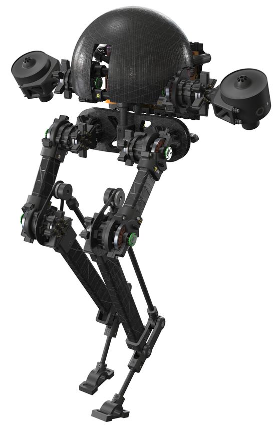
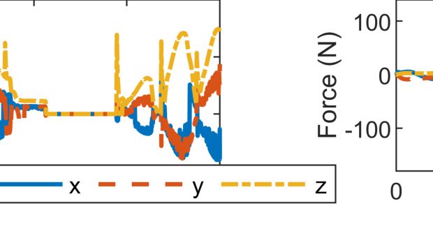
Fig. 5. Shows the simulation result for the walking and jumping maneuvers. (a) Illustrates the stick-diagram plot when the robot walks on flat ground
and jumps over obstacles. (b) Depicts the states evolution, the thrusters action and ground contact forces. Note that the thrusters are employed to stabilize
the frontal dynamics. The RG algorithm is disabled during the ballistic motion (grey area). (c) Close-up view of the constraints at t = [9.5, 11.5]s where
the applied references (xw ) are manipulated such that the constraints (hw (x, xw ) ≥ 0) remain feasible.
simulated using a zero-order hold at a frequency 20 times and kg,d = 268. The frequency of MPC controller applied
smaller than the numerical integration to better capture the in the two-body pendulum model is 100 Hz with a 10
behavior of the onboard computer in Harpy. steps prediction and control horizons. The entire simulation
contains 16 gait cycles (12 s) using the following sequence:
A. Simulation Specifications 3 walking steps, 1 quiet standing cycle, 2 jumping cycles, 4
In this section, all units are in N, kg, m, s. The robot walking steps, 1 quiet standing cycle, 2 jumping cycles, and
has the following dimensions: l1 = [0, 0.1, −0.1]> , l2 = 3 walking steps. The weighting matrices for the MPC are
[0, 0.5, 0]> , l3 = [0, 0, −0.3]> , and l4 = [0, 0.1, 0]> for the We = diag(5, 20), Wu = diag(1/10, 1/10, 1/5), qc = 23◦ ,
left side. The right side simply has the y axis component and the parameters for the jumping trajectories are a = 0.9,
inverted. This gives the robot CoM height of around 0.6 m b = 0.8 for the first jumping cycle, and a = 1.2, b = 0.3 for
for standing and walking. The following mass and inertias the second jump. The ERG is applied using α = 5 which
are used: mB = 2, mH = mK = 0.5, IB = 10−3 , provides a sufficient convergence rate.
IH = IK = 10−4 . Finally, the following ground parameters
are used: µs = 0.6, µc = 0.54, µv = 0.85, kg,p = 8000,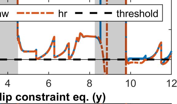
B. Simulation Results and Discussions                                       [3] Y. Gong, R. Hartley, X. Da, A. Hereid, O. Harib, J.-K. Huang, and
                                                                                J. Grizzle, “Feedback control of a cassie bipedal robot: Walking,
   The simulation results can be seen in Fig. 5, where Fig. 5a                  standing, and riding a segway,” in 2019 American Control Conference
shows the key frames of the simulated robot trajectory where                    (ACC), 2019, pp. 4559–4566.
                                                                            [4] M. Hirose and K. Ogawa, “Honda humanoid robots development,”
it walks and jumps over obstacles. Figure 5b shows the data                     Philosophical Transactions of the Royal Society A: Mathematical,
of the thruster forces, ground normal forces, and body states                   Physical and Engineering Sciences, vol. 365, no. 1850, pp. 11–19,
during the simulation. The walking gait designed for a 2D                       2006.
bipedal robot is stable when used in the full 3D system                     [5] W. Kwon et al., “Biped humanoid robot mahru iii,” in IEEE-RAS
                                                                                International Conf. on Humanoid Robots. IEEE, 2007, pp. 583–588.
as the pitch and yaw angles are stabilized by the thruster                  [6] J. E. Pratt et al., “The yobotics-ihmc lower body humanoid robot,” in
actions. Additionally, the trajectory of the body positions                     IEEE/RSJ International Conference on Intelligent Robots and Systems,
match closely towards the desired trajectories throughout                       10 2009, pp. 410–411.
                                                                            [7] H.-W. Park, A. Ramezani, and J. W. Grizzle, “A finite-state ma-
the walking and flight phases. The robot’s pitch angle is                       chine for accommodating unexpected large ground-height variations
uncontrollable as shown in Fig. 5b throughout the entire                        in bipedal robot walking,” IEEE Transactions on Robotics, vol. 29,
simulation. However, the MPC has successfully regulated                         no. 2, pp. 331–345, 2012.
                                                                            [8] B. G. Buss, A. Ramezani, K. A. Hamed, B. A. Griffin, K. S. Galloway,
the foot landing positions such that the foot is positioned                     and J. W. Grizzle, “Preliminary walking experiments with under-
below or in front of the body at the time of landing through                    actuated 3d bipedal robot marlo,” in 2014 IEEE/RSJ International
the appropriate hip sagittal angles, as shown in Fig. 5a.                       Conference on Intelligent Robots and Systems, 2014, pp. 2529–2536.
This allows a smooth transition between landing and walking                 [9] H.-W. Park, K. Sreenath, A. Ramezani, and J. W. Grizzle, “Switching
                                                                                control design for accommodating large step-down disturbances in
which is the primary objective of using the MPC.                                bipedal robot walking,” in 2012 IEEE International Conference on
   The ERG is used to regulate the ground friction forces                       Robotics and Automation, 2012, pp. 45–50.
by manipulating the applied state references during walking                [10] G. Picardi, H. Hauser, C. Laschi, and M. Calisti, “Morphologically
                                                                                induced stability on an underwater legged robot with a deformable
to prevent slips. Figure 5b shows the constraint equation                       body,” The International Journal of Robotics Research, 2019.
values using the applied and target reference (hw and hr                   [11] Y. Kojio et al., “Walking control in water considering reaction forces
respectively), where the target reference trajectories satisfy                  from water for humanoid robots with a waterproof suit,” in 2016
                                                                                IEEE/RSJ International Conference on Intelligent Robots and Systems
the constraints except at around the time range of t =                          (IROS), 2016, pp. 658–665.
[10, 12]s as shown in Fig. 5c. Within this time range, the                 [12] B. Araki, J. Strang, S. Pohorecky, C. Qiu, T. Naegeli, and D. Rus,
desired reference trajectory results in min(hr ) < 0 and the                    “Multi-robot path planning for a swarm of robots that can both fly
                                                                                and drive,” in 2017 IEEE International Conference on Robotics and
ERG has successfully manipulate the applied reference xw                        Automation (ICRA), 2017, pp. 5575–5582.
such that the constraint equation hw ≥ 0 is satisfied. The                 [13] E. Westervelt and J. Grizzle, Feedback Control of Dynamic Bipedal
control output of the ERG is disabled during the jumping                        Robot Locomotion, ser. Control and Automation Series.             CRC
                                                                                PressINC, 2007.
period (shaded gray in Fig. 5b) as the thruster components
                                                                           [14] K. Galloway, K. Sreenath, A. D. Ames, and J. W. Grizzle, “Torque sat-
for position stabilization is handled by the MPC.                               uration in bipedal robotic walking through control lyapunov function-
                                                                                based quadratic programs,” IEEE Access, vol. 3, pp. 323–332, 2015.
           V. C ONCLUSIONS AND F UTURE W ORK                               [15] H. Dai and R. Tedrake, “Planning robust walking motion on uneven
                                                                                terrain via convex optimization,” in IEEE-RAS International Confer-
   The concept design and dynamics simulation of a thruster-                    ence on Humanoid Robots (Humanoids), 11 2016, pp. 579–586.
assisted bipedal robot called Harpy is presented in this paper.            [16] S. Feng, E. Whitman, X. Xinjilefu, and C. G. Atkeson, “Optimization
                                                                                based full body control for the atlas robot,” in IEEE-RAS International
The addition of the thrusters allows the robot to stabilize its                 Conference on Humanoid Robots, 11 2014, pp. 120–127.
frontal dynamics easily and be able to regulate the ground                 [17] A. Ramezani, J. W. Hurst, K. Akbari Hamed, and J. W. Grizzle, “Per-
contact forces directly. To do this, a control algorithm based                  formance analysis and feedback control of atrias, a three-dimensional
                                                                                bipedal robot,” Journal of Dynamic Systems, Measurement, and Con-
on Reference Governors (RGs) was proposed. In addition,                         trol, vol. 136, no. 2, 2014.
the thrusters allowed multimodal locomotion where the robot                [18] A. Ramezani, “Feedback control design for marlo, a 3d-bipedal robot.”
can transition between walking and jumping over obstacles.                      Ph.D. dissertation, 2013.
                                                                           [19] J. Grizzle, A. Ramezani, B. Buss, B. Griffin, K. A. Hamed, and
Through simulations we showed that the integration of the                       K. Galloway, “Progress on controlling marlo, an atrias-series 3d
thrusters can yield a dynamically robust biped. Future work                     underactuated bipedal robot,” Dynamic Walking, 2013.
includes the completion of Harpy. In addition, we will                     [20] P. Dangol, A. Ramezani, and N. Jalili, “Performance satisfaction in
                                                                                midget, a thruster-assisted bipedal robot,” in 2020 American Control
explore the cost of transport in multi-modal systems. Fur-                      Conference (ACC), 2020, pp. 3217–3223.
ther investigations will be made in developing high fidelity               [21] A. C. de Oliveira and A. Ramezani, “Thruster-assisted center man-
models that incorporate realistic thruster dynamics which                       ifold shaping in bipedal legged locomotion,” in 2020 IEEE/ASME
are more appropriate for the real-world implementation of                       International Conference on Advanced Intelligent Mechatronics (AIM).
                                                                                IEEE, 2020, pp. 508–513.
closed-loop feedback on Harpy.                                             [22] P. Dangol and A. Ramezani, “Towards thruster-assisted bipedal loco-
                                                                                motion for enhanced efficiency and robustness,” International Feder-
                           R EFERENCES                                          ation of Automatic Control (IFAC), 2020.
                                                                           [23] A. Hereid, E. A. Cousineau, C. M. Hubicki, and A. D. Ames,
 [1] M. H. Raibert, H. B. Brown Jr, and M. Chepponis, “Experiments in           “3d dynamic walking with underactuated humanoid robots: A direct
     balance with a 3d one-legged hopping machine,” The International           collocation framework for optimizing hybrid zero dynamics,” in 2016
     Journal of Robotics Research, vol. 3, no. 2, pp. 75–92, 1984.              IEEE International Conference on Robotics and Automation (ICRA),
 [2] M. Raibert, K. Blankespoor, G. Nelson, and R. Playter, “Bigdog, the        2016, pp. 1447–1454.
     rough-terrain quadruped robot,” IFAC Proceedings Volumes, vol. 41,    [24] L. Sentis and O. Khatib, “A whole-body control framework for
     no. 2, pp. 10 822–10 825, 2008.                                            humanoids operating in human environments,” in Proceedings 2006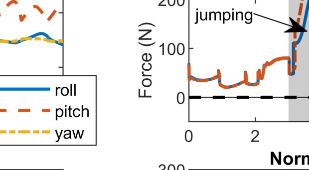
IEEE International Conference on Robotics and Automation, 2006.
       ICRA 2006., 2006, pp. 2641–2648.
[25]   W. B. Powell, Approximate Dynamic Programming: Solving the curses
       of dimensionality. John Wiley & Sons, 2007, vol. 703.
[26]   R. S. Sutton and A. G. Barto, Reinforcement learning: An introduction.
       MIT press, 2018.
[27]   M. Rafieisakhaei, S. Chakravorty, and P. Kumar, “A near-optimal
       decoupling principle for nonlinear stochastic systems arising in robotic
       path planning and control,” in 2017 IEEE 56th Annual Conference on
       Decision and Control (CDC), 2017, pp. 1–6.
[28]   E. D. Sontag, “A lyapunov-like characterization of asymptotic con-
       trollability,” SIAM journal on control and optimization, vol. 21, no. 3,
       pp. 462–471, 1983.
[29]   P. V. Kokotovic, M. Krstic, and I. Kanellakopoulos, “Backstepping to
       passivity: recursive design of adaptive systems,” in IEEE Conference
       on Decision and Control, vol. 4, 12 1992, pp. 3276–3280.
[30]   S. P. Bhat and D. S. Bernstein, “Continuous finite-time stabilization of
       the translational and rotational double integrators,” IEEE Transactions
       on Automatic Control, vol. 43, no. 5, pp. 678–682, 1998.
[31]   E. Garone and M. M. Nicotra, “Explicit reference governor for con-
       strained nonlinear systems,” IEEE Transactions on Automatic Control,
       vol. 61, no. 5, pp. 1379–1384, 2015.
[32]   E. G. Gilbert, I. Kolmanovsky, and Kok Tin Tan, “Nonlinear control
       of discrete-time linear systems with state and control constraints:
       a reference governor with global convergence properties,” in IEEE
       Conference on Decision and Control, vol. 1, 12 1994, pp. 144–149.
[33]   A. Bemporad, “Reference governor for constrained nonlinear systems,”
       IEEE Trans. on Automatic Control, vol. 43, no. 3, pp. 415–419, 1998.
[34]   E. Gilbert and I. Kolmanovsky, “Nonlinear tracking control in the
       presence of state and control constraints: a generalized reference
       governor,” Automatica, vol. 38, no. 12, pp. 2063–2073, 2002.
[35]   H. Khalil, Nonlinear Systems. Pearson Education, Prentice Hall, 2002.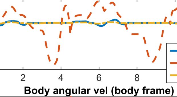
You can also read