Research on Self-balancing Two Wheels Mobile Robot Control System Analysis
←
→
Page content transcription
If your browser does not render page correctly, please read the page content below
Electrical Science & Engineering | Volume 04 | Issue 01 | April 2022

                                                        Electrical Science & Engineering
                                                   https://ojs.bilpublishing.com/index.php/ese

ARTICLE
Research on Self-balancing Two Wheels Mobile Robot Control
System Analysis
Hla Myo Tun1* Myat Su Nwe2 Zaw Min Naing3 Maung Maung Latt4 Devasis Pradhan5
Prasanna Kumar Sahu6
1. Faculty of Electrical and Computer Engineering, Yangon Technological University, Yangon, Myanmar
2. Department of Mechanical Engineering, King Lauk Phya Institute of Technology Myaungmya, Myaungmya,
Myanmar
3. Department of Research and Innovation, Ministry of Science and Technology, Yangon, Myanmar
4. Department of Electronic Engineering, Yangon Technological University, Yangon, Myanmar
5. Department of Electronics & Communication Engineering, Acharya Institute of Technology, Bengaluru, India
6. Department of Electrical Engineering, National Institute of Technology, Rourkela, Odisha, India

ARTICLE INFO                                                   ABSTRACT

Article history                                                The paper presents the research on self-balancing two-wheels mobile robot
Received: 24 January 2022                                      control system analysis with experimental studies. The research problem in
                                                               this work is to stabilize the mobile robot with self-control and to carry the
Revised: 17 March 2022                                         sensitive things without failing in a long span period. The main objective
Accepted: 28 March 2022                                        of this study is to focus on the mathematical modelling of mobile robot
Published Online: 13 April 2022                                from laboratory scale to real world applications. The numerical expression
                                                               with mathematical modelling is very important to control the mobile robot
Keywords:                                                      system with linearization. The fundamental concepts of dynamic system
                                                               stability were utilized for maintaining the stability of the constructed
Mobile robot                                                   mobile robot system. The controller design is also important for checking
Self-balancing robot                                           the stability and the appropriate controller design is proportional, integral,
Control system design                                          and derivative – PID controller and Linear Quadratic Regulator (LQR). The
                                                               steady state error could be reduced by using such kind of PID controller.
PID controller
                                                               The simulation of numerical expression on mathematical modeling was
Dynamic control system analysis                                conducted in MATLAB environments. The confirmation results from
                                                               the simulation techniques were applied to construct the hardware design
                                                               of mobile robot system for practical study. The results from simulation
                                                               approaches and experimental approaches are matched in various kinds of
                                                               analyses. The constructed mobile robot system was designed and analyzed
                                                               in the control system design laboratory of Yangon Technological University
                                                               (YTU).

*Corresponding Author:
Hla Myo Tun,
Faculty of Electrical and Computer Engineering, Yangon Technological University, Yangon, Myanmar;
Email: hlamyotun@ytu.edu.mm

DOI: https: //doi.org/10.30564/ese.v4i1.4398
Copyright © 2022 by the author(s). Published by Bilingual Publishing Co. This is an open access article under the Creative Commons
Attribution-NonCommercial 4.0 International (CC BY-NC 4.0) License. (https://creativecommons.org/licenses/by-nc/4.0/).

                                                                                                                                            7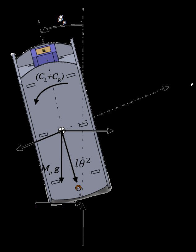
Electrical Science & Engineering | Volume 04 | Issue 01 | April 2022

1. Introduction                                                     people [14]. The general objectives to perform this research
                                                                    are to design and fabricate a relevant balancing two-wheeled
    Mobile robots are empowered for military and indus-             robot chassis, to derive the mathematical model [15] of the
tries and became popular in helping domestic works like a           system, to illustrate the schemes and techniques involved in
four-wheel vacuum cleaner and hospitals like a motorised
                                                                    balancing unstable robotic environments on two wheels using
wheelchair, among those various robots such as a four-wheel
                                                                    proper motors, sensors and a suitable microprocessor, and to
robot, dog robot, spider robot, etc. [1,2]. The two-wheel self-
                                                                    design a complete stable discrete digital control system in the
balancing robot invented by Segway is one of the innovative
                                                                    appropriate software.
robot solutions from personal robotics applications to private
                                                                       In this work, we emphasized the derivation of a mathemat-
transportation. The idea of developing Segway personal
                                                                    ical model based on the inverted pendulum theory, design of
transport, which can balance on its two wheels, has drawn
                                                                    two-wheeled robot in SolidWorks software, implementation
interest from many researchers worldwide. Such kind of
                                                                    of the filter for IMU sensor and PID control, integration of
robot can solve several challenges in industry and society [3-5].
                                                                    the robot’s controller with hardware, and testing, analysing
Because being a small and light cart allows humans to
                                                                    and troubleshooting for the whole system. The authors have
travel in small areas or factories where cars cannot enter
                                                                    solved the stabilizing problem for the mobile robot with
with less pollution and less power consumption. Moreover,
                                                                    self-control and to carry the sensitive things without failing
a Segway robot is interesting because it combines sensory
                                                                    in a long span period. The detailed analyses and numerical
capability and intelligent control methods to keep the robot
                                                                    expression on mathematical modellings were discussed in
in equilibrium [6-8].
                                                                    the following section. The research motivation on the mobile
    The two-wheeled self-balancing robot is similar to the
                                                                    robot system implementation is how to link the simulation
configuration of Segway based on inverted pendulum
                                                                    approaches to experimental approaches in real time
theory. The increasing affordability of commercial off-
the-shelf (COTS) sensing components and microprocessor              applications.
boards has become one of the key reasons to widely                     The paper is organised as follows. Section II presents the
research and report. The two-wheeled self-balancing robot           dynamic mathematical model of the targeted mobile robot.
is a kind of robot that can balance itself on two wheels [9-11].    Section III mentions the control system design. Section IV
This robot chassis was designed in the SolidWorks                   points out the hardware implementation. Section V gives the
software and fabricated with a laser cutter using acrylic           results and discussions on the theoretical and experimental
materials. Then it was mounted on two 12 V DC motors                studies. The last section is the conclusion of the research work.
500 rpm with the encoder. In this project, an inertial
                                                                    2. Mathematical Modelling
measurement unit (IMU) called MPU6050, consisting
of 3 axis accelerometer and a three-axis gyroscope, was                The mathematical modelling for the self-balancing
chosen to measure the robot orientation (roll, pitch, and           mobile robot system could be completed based on the
yaw). It consists of some weak points in the gyroscope              respective section on the dynamical system appraoches.
and accelerometer when they are used alone [12].                    The first portion is concerning the linear model of a DC
    Consequently, the data received from IMU were                   motor for that mobile robot and the second portion is the
converted to the tilt angle and passed through one of the           dynamic model of mobile robot.
filters. A complimentary filter is used for data fusion to get
                                                                    2.1 Linear Model of a Direct Current (DC) Motor
the perfect angle. To balance the device, a controller plays
an essential role in the self-balancing robot. PID controller          Two 500 rpm DC motors are used to power the robot. In
is used in this project to control the speed of the motor           this section, the state-space model of the DC motor, which is
via the PWM duty cycle. The robot’s power can be given              necessary for deriving the balancing robot’s dynamic model,
by using a battery placed on top of the chassis [13]. In this       is expressed. Consequently, the relationship between the
way, the aim of balancing the robot was fully achieved.             input voltage to the motors and the control torque required to
    Because of higher speed due to less friction from fewer         stabilise the robot is obtained.
wheels, more straightforward structural design, lesser                 Figure 1 expresses an effective linear model for a direct
parts that need replacing over time, such as wheels, this           current motor. When a voltage is applied to the dc motor, a
two-wheeled self-balancing robot can be used in various             current (i) is generated. As a result, a motor torque, which
applications with different perspectives such as an intelligent     is proportional to the current, is produced. The equation
gardener in agricultural fields, an autonomous trolley in           can be expressed as
hospitals, shopping malls, offices, airports, healthcare
applications or an intelligent robot to guide blind or disable      τ=
                                                                     m km × i (1)

8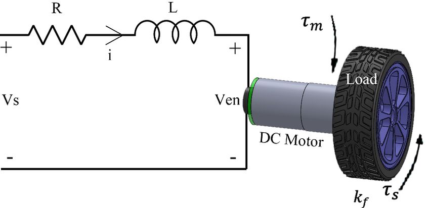
Electrical Science & Engineering | Volume 04 | Issue 01 | April 2022
An electromotive force (emf) is induced when the coil of a d ω km 1
motor is spinning through a magnetic field due to an applied = i − τs (13)
dt IR IR
voltage source. In other words, the motor’s shaft is turning,
and emf is generated when the motor is in an operation By substituting Equation (12) into Equation (13), an
mode. Thus, back emf voltage increases proportionally to the approximation for the DC motor, which is only a function
shaft velocity w, which can be written as of the current motor speed ( ω ), applied voltage ( Vs ) and
Ven= ke × ω (2) applied torque ( τ s ) is obtained.
d ω k m ke 1 1
By using Kirchoff’s Voltage Law, the linear differential = − ω + V s − τ s (14)
dt IR R R IR
equation of the DC motor’s electrical circuit can be written as
di dω k k k 1
−Vs + i × R + L × + Ven =0 (3) − m e ω + m Vs − τ s (15)
=
dt dt IR R IR R IR
di Vs iR Ven A state-space model can represent the dynamic model of
= − − (4)
dt L L L the motor. This state-space consists of two state variables:
di R k V angle ( θ ) and velocity ( ω ). The input variables for the
=− × i − e × ω + s (5)
dt L L L motor is the applied voltage ( Vs ) and applied torque (τ s ).
0 1 0 0
θ θ + k 1
Vs
= k k
0 − m e ω m − τ s
(16)
ω I R R I R R I R
θ V
=y [1 0] + [ 0 0] s (17)
ω
τ s
The outcome of Equation (17) is the estimated mobile
robot position in experimental studies.
Figure 1. Diagram of a DC motor
2.2 Dynamic Modelling of Mobile Robot System
According to Newton’s Law of Motion, the summation
of all torques produced on the shaft is linearly related to This two-wheeled self-balancing robot is a kind of
the acceleration of the shaft by the inertial load of the complex dynamic system because of the nature of an inverted
armature. The motion equation can be written pendulum on a cart. Two equations of motion, which can
∑ M= I R × α (6) completely describe the heart of the balancing robot, are
driven by analysing the robot’s chassis and wheels separately.
∑ M= I R × ω (7) The mathematical model will accommodate such forces
as disturbances, and the motor’s torque can influence the
τ m − k f ω −τ s =
I Rω (8) robot’s behaviour. First of all, the equation of motion
associated with the left and right wheels is obtained. Since
dω the equation for the left and right wheels are absolutely
kmi − k f ω − τ s =
IR (9) analogous, only the equation for the right wheel is given.
dt Figure 2 expresses the free body diagram for both wheels.
d ω km kf 1
= i − ω − τ s (10)
dt IR IR IR
Assume that the motor’s inductance ( L ) and motor’s
friction ( k f ) is approximately zero. Equation (3) and
Equation (10) become Equation (12) and Equation (13),
respectively.
−Vs + iR + Ve =
0 (11)
k 1
− e ω + Vs (12)
i=
R R Figure 2. Free body diagram of the wheels
9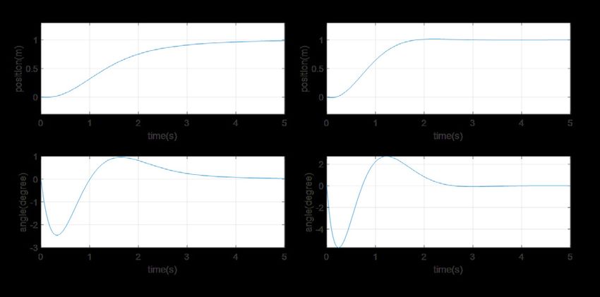
Electrical Science & Engineering | Volume 04 | Issue 01 | April 2022
According to Newton’s law of motion, the summation Equation (28) becomes:
of forces on the horizontal x-direction is For the right wheel,
∑F x = Ma (18)
M w x=
k k k I
− m 2e x + m Vs − w2 x− FR (31)
Rr Rr r
FfR − FR =
M w x(19)
For the left wheel,
Adding the moments about the centroid of the wheel
k k k I
gives Equation (20). M w x=
− m 2e x + m Vs − w2 x− FL (32)
Rr Rr r
∑M O = Iα (20) By adding Equation (31) and Equation (32), the first
equation of motion for the balancing robot is obtained.
I wθw (21)
CR − FfR r =
Iw 2k k 2k
2 M w + − m 2 e x + m Vs − ( FL + FR ) (33)
x =
The motor torque can be expressed from DC motor
r
2
Rr Rr
dynamics, and the equation can be described as,
dω
τ m IR
= + τ s (22)
dt
By rearranging the equation and substituting Equation
(15) into Equation (22), the output torque to the wheels is
attained.
k k k 1
τm =I R − m e θw + m Vs − τ s + τ s (23)
IR R IR R IR
k k k
− m e θw + m Vs (24)
C=
R R
Therefore, Equation (4) becomes
k m ke k m
− θ w + Vs − FfR r =
I wθw (25)
R R
Thus,
k k k I
− m e θw + m Vs − w θw (26)
FfR =
Rr Rr r
The equation of left and right wheels can be obtained
Figure 3. Free Body Diagram of the Chassis
by substituting Equation (26) into Equation (19).
For the right wheel, The free body diagram of the chassis is illustrated in Figure
3. In this figure, the Newton’s law of motion for self-balancing
k k k I
− m e θw + m Vs − w θw − FR (27)
M w x= mobile robot dynamic system based on the mathematical
Rr Rr r
expressions. The mathematical modelling of that free body
For the left wheel, diagram could be evaluated in the following section.
k k k I
− m e θw + m Vs − w θw − FL (28)
M w x= ∑F P = M P x (34)
Rr Rr r
The angular rotation can be converted into linear ( FL + FR ) − M p lθp cos θ p + M p lθ2p sin θ p =
M p x(35)
motion by straightforward transformation because the
The self-motion could be observed by changing the
linear motion is acting on the central point of the wheel.
parameter of “p” for left and right position.
x Thus
θw r =x→ θw = (29)
r ( F=
L
+ FR ) M p lθp cos θ p − M p lθ2p sin θ p + M p x(36)
x Summing the forces perpendicular to the chassis can
θw r =x → θw = (30) also give the second equation of motion for the system.
r
By the linear transformation, Equation (27) and ∑F xp = M p x cos θ p (37)
10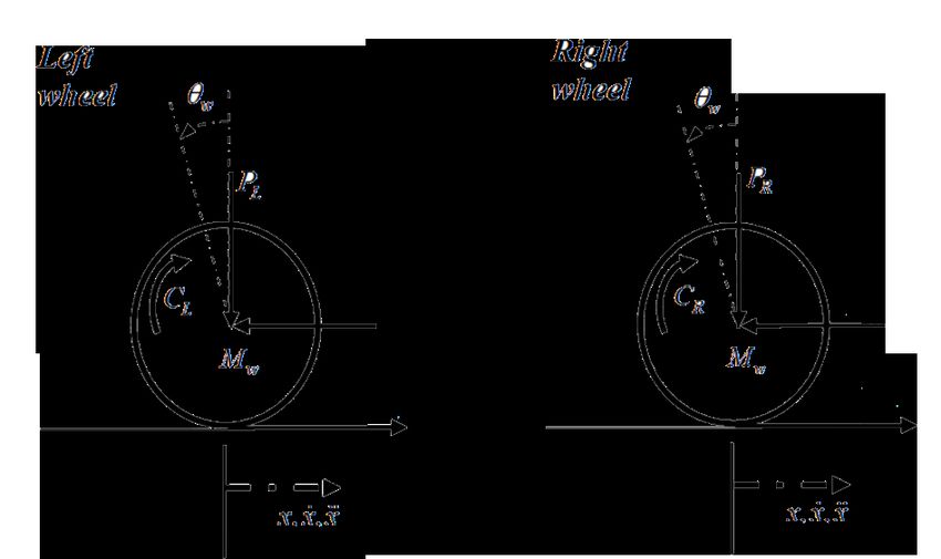
Electrical Science & Engineering | Volume 04 | Issue 01 | April 2022
( FL + FR ) cos θ p + ( PL + PR ) sin θ p 2k k 2k
(38) I p + M p l 2 θp − m e x + m Vs
− M p g cos θ p − M p lθp =
M p x cos θ p Rr R (48)
To get rid of the F and P terms in the above equation,
+ M p l g sin θ p =
− M p lx cos θ p
by summing the moments around the centre of mass of
2lw 2k m ke
chassis, Equation (39) is obtained.
2 M w + r 2 + M p x+ Rr 2 x
(49)
∑M O = Iα (39)
2k m
+ M p lθp cos θ p − M p lθ sin θ p =2
p Vs
− ( FL + FR ) l cos θ p − ( PL + PR ) l sin θ p Rr
(40) The above two equations can be linearised by
− ( CL + CR ) =
I pθp
assuming θ p= π − φ , where φ represents a small angle
The torque applied on the chassis from the motor as from the vertically upward direction. This simplification
defined in Equation (40) and after linear transformation, was used to enable a linear model to be obtained so linear
state space controllers could be implemented.
2k ke 2k
( CL + CR ) =
− m x + m Vs (41) Therefore,
Rr R
cos
= θ p cos (π − φ ) ≈ −1 (50)
Substituting this into Equation (40) gives,
− ( FL + FR ) l cos θ p − ( PL + PR ) l sin θ p sin
= θ p sin (π − φ ) ≈ −φ (51)
2k k 2k (42)
− − m e x + m V =I pθp θp =
φ2 ≈ 0 and θp =
φ(52)
Rr R
The linearised equation of motion is
Thus,
2k k 2k
I p + M p l 2 φ− m e x + m Vs
− ( FL + FR ) l cos θ p − ( PL + PR ) l sin θ p Rr R (53)
2k k 2k (43) − M p lgφ = M p lx
I pθp − m e x + m Vs
=
Rr R
2I w 2k m ke
By multiplying Equation (38) by –l, 2 M w + Rr + M p x+ Rr 2 x
(54)
− ( FL + FR ) l cos θ p + ( PL + PR ) l sin θ p 2 k
(44) − M p lφ= m
Vs
Rr
+ M p l g sin θ p + M p l 2θp =
− M p lx cos θ p
When Equation (53) and Equation (54) are rearranged,
Substitute Equation (43) in Equation (44), the state space equation of the system is obtained.
2k m ke 2k MM pl pl 2k2mkkme ke
I pθp − x + m Vs + M p l g sin θ p =
= φφ x+x+ x x
Rr R (45) ( I(p I+p M+ Mpl pl) ) RrRr( I(p I+p M+ Mpl 2pl)2 )
2 2
(55)
+ M p l 2θp = − M p lx cos θ p 2k2mkm
−−
MM p gl
p gl
V V+ + φφ
R (RI(p I+p M
+Mp l p l) )
2 2 s s
( I(p I+p M+ Mpl 2pl)2 )
To eliminate ( FL + FR ) from the motor dynamics,
Equation (36) is substituted into Equation (16), 2k2mkm
x=
x= VsVs
I 2k k 2k Rr 2 M +2 I2wI w + M
2 M w + w2 x=
− m 2 e x + m Vs Rr 2M w +w 2 2+ M p p
r Rr Rr (46) rr
( )
− M p lθ p cos θ p + M p lθ p sin θ p + M p xR
2
−−
2 k
2km kme ek
x x
Rr 2
2 2M + 2 I2wI w + M (56)
I 2k k 2k Rr 2M w +w 2 2+ M p p
2 M w + w2 x= − m 2 e x + m Vs rr
r Rr Rr (47) M l
M pl p
− M p lθ p cos θ p + M p lθ p sin θ p − M p xR
2
++ I φφ
2
2 M +2 I w w + M
2M w +w 2r 2+ M p p
Rearranging Equation (45) and Equation (46) gives the r
nonlinear equations of motion of the system. By substituting Equation (55) into Equation (49),
11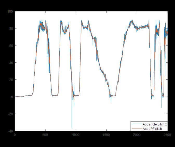
Electrical Science & Engineering | Volume 04 | Issue 01 | April 2022
substituting Equation (43) into Equation (31), and after a cannot maintain its upright position. To hold the robot in
series of algebraic manipulation, the state space equation an excellent place, the controller should know at which
for the system is obtained. angle the robot is tilting. This process can be done by the
IMU sensor, which consists of a three-axis accelerometer
0 0 1 1 0 0 0
0
and a three-axis gyroscope. The accelerometer is
x 2 k k 2(kMk lr( M− Ilr −− MI l− )M l
x 2
) glM gl0 x
M
2 2
x
x 0 0
2 2 2
m e p p p p
responsible for measuring the tilt angle, and the gyroscope
α α x x
m e p p p p
0
= x = Rr α Rr α shows the robot’s angle position. However, each sensor
2
2
φ φ0 0
0 1 φ1 φ data is not entirely accurate due to the presence of noise
0 0
0
φ 2 k k ( r β − M l )
β gl β φ and drift in each sensor. To overcome this problem,
φ0 2k k ( r β − M l )
m e p
M gl M
p
0 φ
a complementary filter is required to implement for
0
m e p p
0
Rr α Rr α α α
2
2
fusing the sensor data. In this robot hardware, a control
0 0 (57) algorithm is written in an intelligent electronic device
2 k ( I + M l − M lr )
2 k ( I + M l − M lr ) known as an Arduino UNO. UNO is used to collect the
2
2
m p p p
m p p p
Rrα Rrα V robot’s orientation in a single axis from the IMU sensor
+
+ 0 V s
s and provide an appropriate control signal to control both
0
left and suitable motor by tuning a Proportional, Integral
2 k (2Mk l(−Mr βl )− r β )
m p
and Derivative (PID) gain value. The output from this
Rrα Rrα
m p
PID controller is a pulse width modulation (PWM) signal.
Consequently, it can control the speed of the motor
x
through a dual full-bridge motor driver (L298N). Thus
1 0 0 0 x
=y + 0 × Vs (58) to balance the two-wheeled self-balancing robot, tuning
0 0 1 0 φ
the PID gain values and filtering the sensor data play an
φ
essential role in this unstable system.
Where,
I w
3.2 Closed-loop PID Controller Testing Based on
α=
I p β + 2M pl M w +
2
(59) Mathematical Model
r 2
PID controller is simulated in MATLAB/SIMULINK
2I
β = 2 M w + 2w + M p (60) using the accurate parameter in the robot’s mathematical
r
model. The mathematical model equation was driven in
The detail descriptions for all mathematical expression Equation (56), and the robot’s precise parameters have
are offered in the background theory of mobile robot been calculated in section III.
system in several books. Figure 4 demonstrates the Closed Loop Impulse
In the abovementioned model, it is assumed that the Response of the System with PID. This simulation is
wheels of the vehicle will always stay in contact with the constructed according to the state-space model. An
ground and that there is no slip at the wheels. Therefore, impulse response is used to test the PID closed-loop
cornering forces are also considered negligible. control system. The first proportional gain (K p=15)
controls the position of the robot and the second PID
3. Experimental Results and Discussions controller controls the robot’s angle. The input source is
an impulse signal, and it is similar to the robot, which
The experimental results based on separated hardware
is suddenly pushed in the objective case. This impulse
implementation and overall system implementation
force will cause the robot to change its stable position
were presented in this section. And also the outcomes
and angle for a short period. The result can be seen in
of research are mentioned based on the discussions on
Figure 5.
several analyses. Figure 5(a) means that the robot’s position has changed
from 0 meters to around 0.8 meters first due to the applied
3.1 Overall Operation of the System
impulse force. This will create the robot to lean nearly
The self-balancing two-wheeled robot is based on an 18 degrees. Consequently, the robot’s angle must be
inverted pendulum theory. Without any control system, it controlled with proper PID gain values to maintain its
12Electrical Science & Engineering | Volume 04 | Issue 01 | April 2022
stability. Unless the robot’s angle is held, it will fall. With
the help of PID controllers in both position and angle,
the robot will return to its initial position after 2 seconds,
and at the same time, the robot’s tilting angle will return
to zero degrees. Among these two Figures 5(a) and 5(b),
the right-hand side graph can give a better result when
the robot’s displacement and tilt angle measurements are
compared.
In the second experiment, a unit step signal is used as
an input to the system, and then the robot’s position and
angle are checked after passing through the PID controller
in both cases. The main unsimilar point between Figure
4 and Figure 6 is the input signal. Figure 4 uses an
impulse signal, while Figure 6 uses a unit step signal. The
simulation result can be demonstrated in Figure 7. This
time let’s assume that the user wants to move the robot to
one meter and stay in that position, like giving a unit step
function to the robot’s position in the simulation. In order
to observe this, the robot should lean for at most around
15 degrees. With the help of these PID gain values, the
robot could manage to reach that set point position within
3 seconds. After getting to the desired position, the robot’s
tilting angle will be returned to zero. In other words, the
robot will return to its balanced position. Among these,
two graphs the right-hand side graph can give a better
result.
Last but not least, the PID controller is used to control
only the robot’s angle instead of the robot’s position.
MATLAB simulation diagram is shown in Figure 8.
This phenomenon is quite similar to setting the robot to
lean forward to a certain degree constantly. The simulation
result can be seen in Figure 9. In this simulation, the robot
is set to lean forward for one degree constantly. Thus
in Figure 9, at first, the robot is oscillating and trying to
maintain in one degree; as a result, the robot will move
continuously. Therefore, between these two figures: Figure Figure 4. Closed Loop Impulse Response of the System
9(a) and Figure 9(b), Figure 9(b) can be assumed to be the with PID
best one by comparing the robot’s angle graph.
One of the interesting facts in this simulation test is
that all the PID gain values that are used in those three
different simulations are the same value. This means that
appropriate PID gain values for both unit step and unit
impulse function in controlling both position and angle
have already been tuned after realising the characteristic
of the PID controller and trying a try and error method for
tuning the gain values. Moreover, PID gain values used
in every simulation (a) can balance the robot in software Figure 5. Test and Result of Closed Loop Impulse
simulation and hardware testing. Response with PID Controller in Both Position and Angle
13Electrical Science & Engineering | Volume 04 | Issue 01 | April 2022
Figure 8. Closed Loop Unit Step Response of the System
with PID Controller in Angle
Figure 6. Closed Loop Unit Step Response of the System
with PID Controller in Both Position and Angle
Figure 9. Test and Result of Closed Loop Unit Step
Response with PID controller in Both Position and Angle
3.3 Closed Loop LQR Controller Testing Based
on Mathematical Model
After substituting the robot’s parameter into the state-
Figure 7. Test and Result of Closed Loop Unit Step space model derived in section III, Equation (60) is
Response with PID controller in Both Position and Angle obtained.
14Electrical Science & Engineering | Volume 04 | Issue 01 | April 2022
x 0 1 0 0 x 0 LQR simulation result (b) with the PID control simulation
x 0 −113 10.81 0 x 4.296 result in Figure 7(b), the LQR controller can perform
+ Vs (61) better because the robot will reach the desired distance of
φ 0 0 0 1 φ 0
1 meter within 2 seconds the tilting angle of a maximum
φ 0 −630.4 178.2 0 φ 23.96 5 degrees. But with the PID control, the robot needs to tilt
For a linear control system to be implemented, the about 15 degrees to reach the desired position within 2
system has to be controllable. This requires that the rank seconds.
of the n × n controllability matrix C = BAB... A B is n
n −1
3.4 Flowchart of the Robot Control System
or modulus of C is not equal to zero.
The algebraic Ricatti equation is solved using The flowchart used to carry this project can be seen
MATLAB, and the control gain K is evaluated for in Figure 11. Once the necessary components are set,
different values of Q and R weighting matrices. The the operation of the flowchart will be explained in this
response of the system is simulated as well. section.
The Q matrix assumes the form of
Start
a 0 0 0
0 b 0 0 Setup
Q= (62) MPU6050
0 0 c 0
0 0 0 d Read Angle from Gyroscope
and Accelerometer
where the values of a, b, c and d are the weightings for
the states x, x, φ , φwhile the weighing matrix R is a scalar Perform a Complementary
value as there is only one control input to the system. The Filter
values in Q and R matrices are adjusted to penalise the
Compute PID Controller Gain
system state space and input. The main aim of this control
system is to make the states of the system converge
to zero at the shortest time possible. Thus the control Does Robot
Balance?
engineer should adjust the Q and R matrices to obtain
the desired response. The simulation result for this self-
balancing robot is illustrated in Figure 10.
Speed=Output of PID Speed=0
Control the Motor
Does Robot Arrive
Desired Loaction?
Figure 10. Test and Result of Closed Loop LQR controller End
Figure 10(a) uses a=10, b=10, c=60, d=100 for Q
Figure 11. Flowchart of the Robot Control System
matrix and R=0.001. Using these values, the robot
will reach the desired position 1m after 4 seconds by First of all, the MPU6050 sensor is initialised in
oscillating the robot between –2 degrees and 1 degree. the setup function. After that, the accelerometer and
Figure 10(b) uses a=100, b=10, c=600, d=100 for Q gyroscope raw data are acquired from the sensor and then
matrix and R=0.001. At these values, the robot will reach passed through the complementary filter to remove drift
the desired position 1 m after 2 seconds by oscillating the and noise from MPU6050. Then, it is sent to the PID
robot between –5 degrees and 2.3 degrees. Among these controller. By tuning the PID gain values, the motor speed
two LQR simulations, Figure 10(b) can provide better can be controlled with a PWM signal. If the sensor senses
performance than that of (a). Moreover, by comparing this that the robot is in a balanced condition, the PID controller
15Electrical Science & Engineering | Volume 04 | Issue 01 | April 2022
will command the motor not to move for ten milliseconds gradually. However, in the filtered data, a small drift still
which becomes the system’s loop time. When the sensor presents in between 2000 and 2500 samples.
senses that the robot is tilting forward for five degrees, the
PID controller will command the motor to accelerate the
motor forward until the robot becomes stable. In this way,
the robot can balance itself successfully. Finally, when
battery power is not enough, the robot will stop running [16].
The specific coding is not mentioned in this paper.
3.5 Hardware Testing
To implement the flowchart program in the hardware
properly. Getting angle from the MPU6050 sensor is the
first priority for hardware testing.
The Arduino Uno communicates with the MPU6050
through the I2C protocol. Thus serial clock pin (SCL) is
connected to the Arduino (A5) pin as well as the serial
data pin (SDA) is connected to the Arduino (A4) pin. Figure 13. Accelerometer Pitch Angle
The sensor’s interrupt pin (INT) is then connected to the
Arduino pin2. Arduino supplies 3.3V to the sensor by Figure 13 represents the nature of the accelerometer
connecting the Vcc pin from the sensor and the 3V3 pin sensor. The blue line represents the accelerometer pitch
from the Arduino. The two ground pins are made sure to angle, and the red line represents the accelerometer
communicate with each other. low pass filter pitch angle. Even there is no bias in the
After interfacing the sensor and Arduino Uno, accelerometer, and it is pretty sensitive to noise. As a
the program should be uploaded to test the sensor. result, a low pass filter is needed to filter out this noise.
Then the raw data are saved in the excel file and Moreover, even the sensor is rotated from 0 to 90 degrees
for six times, the accelerometer sensor data and low pass
plotted in MATLAB. After that, check the nature of
filtered data cannot represent absolute 90 degrees when
the accelerometer and gyroscope sensor and perform
only the accelerometer sensor is used to calculate the
complementary in MATLAB code.
angle.
Figure 12. Gyroscope Pitch Angle
The sensor is rotated only in one axis (pitch angle) Figure 14. Complementary Filter Pitch Angle
from 0 to 90 degrees and then rotates again from 0 to In order to solve the problem occurring in both ac-
90 degrees for another four times. In Figure 12, the celerometer and gyroscope sensors, a complementary
blue line represents the gyroscope pitch angle, and the filter is used to get a better result. For example, Figure 14
red line represents the gyroscope high pass filter pitch combines the two sensors’ data, and this filter is designed
angle. It was evident that the gyroscope has a bias. Thus to trust the gyroscope sensor data more than that of the
without passing a high pass filter, the sensor data are drift accelerometer.
16Electrical Science & Engineering | Volume 04 | Issue 01 | April 2022
3.6 Implementing PID Controller to the Robot result, the PID controller needs to work at a maximum and
Control System a minimum limit of +255 and –255 PWM signals during
the running condition. However, it cannot maintain the
After testing each component before implementing the
robot in a stable condition.
whole system, the PID control algorithm is written in the
Arduino. This PID controller plays an essential role in the
self-balancing robot system. The reason is that without
a controller or a poor control design, the robot cannot
balance itself and is stable in one position. Thus, in this
case, tuning the PID controller plays an important role.
Therefore, the author did a lot of experiences to get the
perfect controller gain values. Among them, four different
PID gain values are selected.
Figure 17. The Third PID Tuning in Robot
Thirdly, PID gain value is changed into Kp = 28, Ki =
200, and Kd = 2. Then the robot’s condition is checked.
Unlike Figure 16, the PID controller does not need to
work at a maximum or minimum limit apart from a
disturbance. These gain values can keep the robot in a
stable condition since, in Figure 17(b), the robot does not
Figure 15. The First PID Tuning in Robot tilt a lot without a disturbance.
Figure 15 shows all data conditions of the running
robot with PID gain values of Kp = 50, Ki = 200 and Kd =
10. Figure 14(a) represents the PID output (PWM signal)
to control the motor speed. Figure 14(b) illustrates the
robot’s actual tilting angle. In this Figure 14, the robot
cannot keep in a balance position because it falls down
after operating for a short period. This phenomenon can
be seen when the robot’s tilting angle reaches 90 degrees.
Figure 18. The Balancing Condition of the Robot in
Upright Position
Figure 16. The Second PID Tuning in Robot
This final PID gain value of Kp = 24.69, Ki = 218.4; and
Since PID gain values in Figure 14 cannot maintain
the robot in an upright position, other PID gain values Kd = 1.924 can improve the robot’s stability. The robot
are tuned. Figure 16 shows all data conditions of the oscillates between –3 degrees and 3 degrees during the
running robot with PID gain values of Kp = 103.571, Ki = experiment. This means that the PID controller controls
129.5501, and Kd = 20.7004. Figure 15(a) represents the the motor driver not to let the robot tilt beyond 3 degrees.
PID output (PWM signal) to control the motor speed. Thus it can be concluded that this gain value can provide
Figure 16(b) illustrates the robot’s actual tilting angle. a more stable condition for the self-balancing robot. The
These gain values make the robot oscillate a lot; as a result can be seen in Figure 18.
17Electrical Science & Engineering | Volume 04 | Issue 01 | April 2022
hardware testing, only PID controller is used. First, the
3D design of the self-balancing robot was drawn in the
Solid Works software to find the best location for each
electronic component. By doing so, the author does not
have any problem with hardware assembling in practice.
Next, the complementary filter has been successfully
implemented to filter a gyroscope drift and accelerometer
noise, allowing for an accurate estimation of the robot’s
tilting angle. Arduino must communicate the IMU sensor
via I2C communication and control the motor’s speed via
PWM signal. After passing the filtered sensor data to the
microcontroller, the microcontroller compares the actual
tilting angle with the setpoint value to check the error.
This error is compensated by using a PID controller in
Figure 19. The Balancing Condition of the Robot in the hardware. Both PID and LQR control algorithms have
Presence of Extra Weight successfully compared the software simulation result in
MATLAB using the robot’s state-space model. LQR can
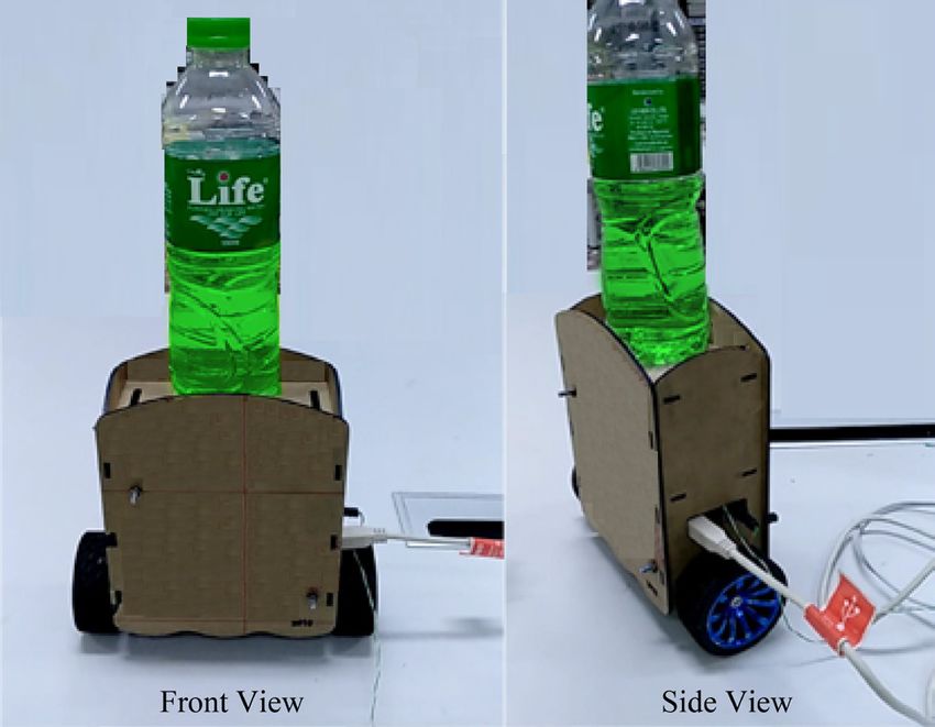
Moreover, to know whether this PID gain value of Kp =
provide better performance than the PID controller. Due
24.69, Ki = 218.4; and Kd = 1.924 can maintain the robot’s
to the time limit, only the PID controller is successfully
stable condition or not when extra weight is applied to
implemented to address the problem of balancing an
it, a half-filled 0.6 litre of water bottle is placed at the
unstable system in hardware testing. But this PID tuned
top of the robot’s chassis and run the robot. Therefore,
values of Kp = 24.69, Ki = 218.4, and Kd = 1.924 used in
this PID controller can also maintain the robot in a
hardware can maintain the robot upright on flat surfaces.
stable condition. The front and side view of the robot’s
Moreover, it can control the robot in a balanced condition
running condition can be seen in Figure 19. In order to
with extra weight, as shown in Figure 18. Last but not least,
get this PID to gain value, many experiments are tested
this gain value is also satisfied in software simulation.
during the research program. The simulation tools in this
mathematical modelling are based on the MATLAB and Therefore, many experiments and simulations were done
Arduino programming. The accuracy could be checked to achieve a better result. This work is novel for empha-
by using the ratio of difference between real and defined sizing on the numerical approaches for experimental ap-
position to the defined position in this study. proaches with discrete components and utilizing the fun-
damental concepts of the dynamic control system design.
3.7 Challenging Issues The performance comparison on the mobile robot system
was depending on the controller design and robustness of
During this research, a minor challenging issue
the system. That is the innovative work in this study.
appeared, such as resizing the depth of the robot chassis
because the laser cutter cuts the acrylic sheets into 2 3.9 Limitations
mm instead of cutting into 3mm sheets. However, one
major issue was found with the DC motors employed: the The limitations of the developed mobile robot system
first motor, GM25-370-24140 DC motor, does not have are latency of the control signal input to the process by
enough RPM to rotate when the robot turns to tilt into a controller output and the translational vector between the
large angle. For this reason, it is so complicated to tune simulation approaches to experimental approaches. The
the PID control. Fortunately, this problem is solved by problem could be solved to acquire the better performance
replacing it with a 500RPM DC motor. for experimental studies with the speed of controller
design and optimal gain tuning is the contribution in this
3.8 Discussions work.
This research work successfully achieves the goals
4. Statistics Table for Results Comparison
of balancing unstable two-wheeled robots. Balancing an
unstable system is a challenging problem in the research The experimental results of self-balancing mobile
field, and the various controllers can be used in stabilising robot system in this study and recent works are given in
the system. In this research work, PID and LQR controller the following Table 1. The performance comparisons are
is used to control the robot’s position and angle. But in found in this table with various kinds of conditions.
18Electrical Science & Engineering | Volume 04 | Issue 01 | April 2022
Table 1. Performance Comparison Table or counter-clockwise direction via Bluetooth wireless
Controller Performance
connection can also be considered in this self-balancing
Works Accuracy Robustness robot. The numerical expressions were matched to the
Design Level
[17] PD 93% High Satisfy experimental studies in this study based on the accuracy
[18] LQR 94% High Satisfy
percentage of 98%. The performance level is also very
high by comparing with the other recent works.
[19] PWM 90% Medium Satisfy
This
PID and LQR 98% Very High Satisfy Conflict of Interest
Work
There is no conflict of interest.
The control algorithm is based on the real time control
system for specific analysis. The application of the Acknowledgment
mobile robot system is for healthcare service in real time
conditions. The authors acknowledge researchers and colleagues
from the Faculty of Electrical and Computer Engineering
5. Conclusions of Yangon Technological University. This work is fully
supported by Government Research Funds for 2021-
This research successfully achieved its aims to balance
2022 Academic Year. This work is completely measured
a self-balancing robot based on the inverted pendulum
and analyzed at the Electrical and Electronics Properties
model. Two control strategies have been implemented to
Evaluation Laboratory Room (EB-402) of the Myanmar
address the problem of balance control for the system.
Japan Technological Development Centre 1 (MJTDC 1)
The gain matrices obtained from PID simulation are
of Yangon Technological University (YTU). This work
implemented in this self-balancing robot for real-time
is collaborative research work with Acharya Institute of
controller experimentation. During the testing, the robot
Technology in India and Chulalongkorn University in
can maintain its vertical position by slightly adjusting
Thailand.
its wheels. Besides PID control, the LQR controller is
also successfully tested in MATLAB simulation. The References
PID controller can easily be tuned by observing the
optimal condition. The LQR controller can also better [1] Peng, K., Ruan, X., Zuo, G., 2012. Dynamic model
results when the Q matrix and R matrix are adequately and balancing control for two-wheeled self-balancing
set. Many simulations are run to get the best result for mobile robot on the slopes. Proceedings of the 10th
this self-balancing robot. In the hardware testing, the World Congress on Intelligent Control and Automa-
PID controller is designed to control a single axis robot tion. pp. 3681-3685. (Accessed 9 September 2021).
tilting angle, y-axis. Rotating in both x and z axes is DOI: https://doi.org/10.1109/WCICA.2012.6359086
neglected in implementing the PID control algorithm [2] Bin, H., Zhen, L.W., Feng, L.H., 2010. The Kinemat-
because this research work focuses only on stabilizing the ics Model of a Two-Wheeled Self-Balancing Autono-
robot. Also, controlling the position is not considered in mous Mobile Robot and Its Simulation. 2010 Second
hardware testing. However, in MATLAB simulation, both International Conference on Computer Engineering
PID and LQR are considered in controlling both robot’s and Applications. pp. 64-68. (Accessed 18 September
position and angle. Thus, considering the yaw axis and 2021).
x y movement is recommended for trajectory tracking in DOI: https://doi.org/10.1109/ICCEA.2010.169
the robot’s hardware. So that later formation control can [3] Gong, D., Li, X., 2013. Dynamics modeling and
be performed. Stabilizing the robot on a sloped area and a controller design for a self-balancing unicycle robot.
rough surface area is recommended as a further extension. Proceedings of the 32nd Chinese Control Confer-
PID controller cannot maintain stable conditions for ence. pp. 3205-3209. (Accessed 27 September 2021).
slopes and rough surfaces. Thus apart from PID controller, [4] Nikita, T., Prajwal, K.T., 2021. PID Controller Based
Linear Quadratic Regulator (LQR), pole-placement, Two Wheeled Self Balancing Robot. 2021 5th In-
fuzzy control, adaptive control, sliding mode control ternational Conference on Trends in Electronics and
(SMC), etc., are recommended to implement in this robot Informatics (ICOEI). pp. 1-4. (Accessed 8 October
to decide which controller can perform the best in the 2021).
future development of the self-balancing robot. Moreover, DOI: https://doi.org/10.1109/ICOEI51242.2021.9453091
a manual remote control system like commanding the [5] Philip, E., Golluri, S., 2020. Implementation of an
robot to move forward, backwards and rotate clockwise Autonomous Self-Balancing Robot Using Cascaded
19Electrical Science & Engineering | Volume 04 | Issue 01 | April 2022
PID Strategy. 2020 6th International Conference on DOI: https://doi.org/10.1109/CCDC.2009.5192771
Control, Automation and Robotics (ICCAR). pp. 74- [13] Kongratana, V., Gulphanich, S., Tipsuwanporn, V., et
79. (Accessed 9 September 2021). al., 2012. Servo state feedback control of the self bal-
DOI: https://doi.org/10.1109/ICCAR49639.2020.9108049 ancing robot using MATLAB. 2012 12th Internation-
[6] Jianwei and Xiaogang, 2008. The LQR control and al Conference on Control, Automation and Systems.
design of dual-wheel upright self-balance Robot,” pp. 414-417. (Accessed 9 September 2021).
2008 7th World Congress on Intelligent Control and [14] Gong, Y., Wu, X., Ma, H., 2015. Research on Con-
Automation. pp. 4864-4869. (Accessed 9 September trol Strategy of Two-Wheeled Self-Balancing Robot.
2021). 2015 International Conference on Computer Science
DOI: https://doi.org/10.1109/WCICA.2008.4593712 and Mechanical Automation (CSMA). pp. 281-284.
[7] Yu, N., Li, Y., Ruan, X., et al., 2013. Research on at- (Accessed 9 September 2021).
titude estimation of small self-balancing two-wheeled DOI: https://doi.org/10.1109/CSMA.2015.63
robot. Proceedings of the 32nd Chinese Control [15] Tun, H.M., Nwe, M.S., Naing, Z.M., 2008. Design
Conference. pp. 5872-5876. (Accessed 9 September analysis of phase lead compensation for typical laser
2021). guided missile control system using MATLAB bode
[8] Putov, A.V., Ilatovskaya, E.V., Kopichev, M.M., plots. 2008 10th International Conference on Control,
2021. Self-balancing Robot Autonomous Control Automation, Robotics and Vision. pp. 2332-2336.
System. 2021 10th Mediterranean Conference on (Accessed 9 September 2021).
Embedded Computing (MECO). pp. 1-4. (Accessed DOI: https://doi.org/10.1109/ICARCV.2008.4795897
9 September 2021). [16] Tun, H.M., Nwe, M.S., Naing, Z.M., et al., 2022.
DOI: https://doi.org/10.1109/MECO52532.2021.9459720 “Sliding Mode Control-Based Two Wheels Mobile
[9] Sarathy, S., Mariyam Hibah, M.M., Anusooya, S., et Robot System”, The 14th Regional Conference on
al., 2018. Implementation of Efficient Self Balanc- Electrical and Electronics Engineering (RC-EEE
ing Robot. 2018 International Conference on Recent 2021), Chulalongkorn University, Thailand. (Ac-
Trends in Electrical, Control and Communication cessed 9 January 2022).
(RTECC). pp. 65-70. (Accessed 9 September 2021). [17] Velagic, J., Kovac, I., Panjevic, A., et al., 2021. De-
DOI: https://doi.org/10.1109/RTECC.2018.8625624 sign and Control of Two-Wheeled and Self-Balanc-
[10] Sun, W.X., Chen, W., 2017. Simulation and debug- ing Mobile Robot. pp. 77-82.
ging of LQR control for two-wheeled self-balanced DOI: https://doi.org/10.1109/ELMAR52657.2021.
robot. 2017 Chinese Automation Congress (CAC). 9550938
pp. 2391-2395. (Accessed 9 September 2021). [18] Pajaziti, A., Gara, L., 2019. Navigation of Self-Bal-
DOI: https://doi.org/10.1109/CAC.2017.8243176 ancing Mobile Robot Through Sensors. IFAC Papers
[11] Ruan, X.G., Liu, J., Di, H.J., et al., 2008. Design and Online. 52-25, 429-434.
LQ Control of a two-wheeled self-balancing robot. DOI: https://doi.org/10.1016/j.ifacol.2019.12.576
2008 27th Chinese Control Conference. pp. 275-279. [19] Chhotray, A., Pradhan, M.K., Pandey, K.K., et
(Accessed 9 September 2021). al., 2016. Kinematic Analysis of a Two-Wheeled
DOI: https://doi.org/10.1109/CHICC.2008.4605775 Self-Balancing Mobile Robot. Proceedings of the
[12] Lv, Q., Wang, K.K., Wang, G.Sh., 2009. Research of International Conference on Signal, Networks, Com-
LQR controller based on Two-wheeled self-balancing puting, and Systems, Lecture Notes in Electrical En-
robot. 2009 Chinese Control and Decision Confer- gineering. Springer India. 396.
ence. pp. 2343-2348. (Accessed 9 September 2021). DOI: https://doi.org/10.1007/978-81-322-3589-7_9
20You can also read