Rendering Nighttime Image Via Cascaded Color and Brightness Compensation
←
→
Page content transcription
If your browser does not render page correctly, please read the page content below
Rendering Nighttime Image Via Cascaded Color and Brightness Compensation

                                                                                            Zhihao Li, Si Yi, and Zhan Ma*

                                                                     Abstract
arXiv:2204.08970v2 [cs.CV] 21 Apr 2022

                                             Image signal processing (ISP) is crucial for camera
                                         imaging, and neural networks (NN) solutions are exten-
                                         sively deployed for daytime scenes. The lack of sufficient
                                         nighttime image dataset and insights on nighttime illumina-
                                         tion characteristics poses a great challenge for high-quality
                                         rendering using existing NN ISPs. To tackle it, we first
                                         built a high-resolution nighttime RAW-RGB (NR2R) dataset
                                         with white balance and tone mapping annotated by expert
                                         professionals. Meanwhile, to best capture the character-
                                         istics of nighttime illumination light sources, we develop
                                         the CBUnet, a two-stage NN ISP to cascade the compensa-
                                         tion of color and brightness attributes. Experiments show
                                         that our method has better visual quality compared to tradi-
                                         tional ISP pipeline, and is ranked at the second place in the
                                         NTIRE 2022 Night Photography Rendering Challenge [13]
                                         for two tracks by respective People’s and Professional Pho-
                                         tographer’s choices. The code and relevant materials are
                                         avaiable on our website1 .

                                         1. Introduction
                                             As for camera imaging, photons first converge on the                      Figure 1. Nighttime RAW image (visualized) and the correspond-
                                         sensor chip to generate the raw electrical image (RAW)                        ing RGB image processed rened by the proposed CBUnet.
                                         reflecting acquired scene; And then the image signal pro-
                                         cessor (ISP) is usually devised to transform camera RAW
                                         image to corresponding RGB representation pleasantly per-                     systems in ISP exemplified previously are developed sepa-
                                         ceivable to human visual system (HVS). Therefore, the ef-                     rately, usually taking into account the characteristics of un-
                                         ficiency of ISP is of great importance for the generation of                  derlying sensor and optics for systematic optimization.
                                         high-quality RGB images used in vast applications.                               In practice, the HVS can efficiently render dynamic
                                             Traditional ISP systems usually include demosaicing,                      scenes because of the priors in brain memory [25, 38]
                                         automatic white balance (AWB), color space conversion,                        (e.g., background illumination, environment understand-
                                         tone mapping, denoising, compression, etc. Among them,                        ing), which however is difficult for traditional ISPs to cap-
                                         most steps aim at alleviating or eliminating the inherent de-                 ture due to the lack of understanding of scene. Therefore,
                                         fects incurred by the image sensor and environment to ren-                    some recent studies [5, 6, 28] have tried to use neural net-
                                         der high-quality images in terms of the color, brightness,                    works (NN) to replace some modules in ISP to dynami-
                                         texture sharpness, dynamic range, etc. for visually pleasant                  cally adjust the output RGB image with scene priors ac-
                                         presentation to HVS perception. Oftentimes, modular sub-                      cordingly. For example, Bianco et al. [6] presented a three-
                                                                                                                       stage CNN model method to do illuminant estimation of
                                            * Z. Li (lizhihao6@outlook.com) and Z. Ma (mazhan@nju.edu.cn)
                                         are with Nanjing University, Jiangsu 210093, China; And S. Yi
                                                                                                                       RAW images. Panetta et al. [28] proposed a deep learning-
                                         (1811326@mail.nankai.edu.cn) is with Nankai University, Tianjin, China.       based tone mapping operator (TMO-Net), which offered a
                                            1 https://njuvision.github.io/CBUnet                                       generalized, efficient and parameter-free way across a wider

                                                                                                                   1
Rank                     Unlike daytime images mostly with high illumination,
    Team No.      #Votes    Mean Score      People Pro.                nighttime images were typically acquired under the illumi-
    Team1          2603      0.8009            1       1               nation conditions with complex light sources. We proposed
    Ours           2047      0.6298            2       2               a two-stage CBUnet to cascade the processing of the color
    Team3          1979      0.6089            3       3               and brightness compensation where we used a Unet [32]
    Team4          1964      0.6045            4       4               with channel-attention for color correction at the first stage,
    Team5          1935      0.5955            5       6               and in the second stage we applied a histogram-aware Unet
    Team6          1866      0.5742            6       7               for tone mapping by leveraging statistical brightness infor-
    Team7          1559      0.4798            7       8               mation from nighttime images.
    Team8          1505      0.4631            8       9                  Our main contributions can be summarized as follows:
    Team9          1433      0.4411            9      10
    Team10         1288      0.3965           10       5                  • A high-resolution image dataset with nighttime RAW-
                                                                            RGB (NR2R) pairs that are rendered and annotated by
Table 1. Result Illustration of Number of Votes (#Votes), Mean              experts with white balance and tone mapping is pro-
Score, Rank of respective People and Professional Photographer’s            vided.
choice for NTIRE 2022 Night Photography Rendering Challenge.
                                                                          • A novel two-stage CBUnet to compensate color and
                                                                            brightness attributes consecutively is developed to ren-
spectrum of HDR (high dynamic range) content. Moreover,                     der acquired RAW images.
there had been other works [18–20] that attempted to re-
                                                                          • As shown in Table 1, our CBUnet achieved the second
place the entire ISP system with an end-to-end trainable
                                                                            best performance in both people’s and photographer
neural network.
                                                                            choice of IEEE CVPR NTIRE 2022 Night Photogra-
   Training a robust NN ISP, e.g., either modular function                  phy Rendering Challenge.
or end-to-end system, required a great amount of paired
data, and then significant manpower and resources were
                                                                       2. Related Work
devoted to build proper datasets. However, most exiting
datasets were collected at daytime, making it not be appli-                Over past decades, modular subsystems of a camera
cable for applications in the night because of the great illu-         ISP system had been extensively examined like the de-
mination variations between daytime and nighttime. Taking              mosaicing [11, 17, 24], denoising [7, 9, 14], white balanc-
the AWB as an example, daytime light sources are primar-               ing [8, 15, 36], tone mapping [22, 33, 36], etc. Most ISP
ily strong sunlight, while nighttime light sources are more            subsystems had been successfully emulated and enhanced
complex, including a variety of artificial light sources that          using deep learning techniques by carefully modeling asso-
have never appeared in existing daytime datasets.                      ciated function as the image-to-image translation problems.
   To address the lack of paired RAW-RGB data captured                     Demosaicing refers to restoring the color information of
at night time, we labeled a high-resolution nighttime RAW              the remaining two channels of each pixel through interpo-
to RGB (NR2R) dataset. Specifically, we selected and de-               lation. Park et al. applied residual learning and densely
noised 150 RAW images with a resolution of 3464×5202                   connected convolutional neural network to do color filter
from the training and validation set provided by the night             array demosaicking, where the proposed model did not re-
image rendering challenge [13]. Then, we first converted               quire any initial interpolation step for mosaicked input im-
the RAW sample to its corresponding RGB format by a sim-               ages [29].
ple ISP for extracting the white patch manually. The white                 Denoising aims to remove the noise and recover the la-
patch of each converted RGB image was used to estimate                 tent observation from the given noisy image. Zhang et al.
the ground truth illumination for subsequent AWB. Later                proposed a depth image denoising and enhancement frame-
then, the denoised RAW image was fed through a serial op-              work using a lightweight convolutional network [40] where
erations including bilinear demosaicing, auto white balance            a three-layer network model was applied for high dimension
with label white balance, color space correction with cam-             projection, missing data completion and image reconstruc-
era inner color correction matrix (CCM) and neural network             tion. Zhou et al. proposed a novel Bi-channel Convolutional
based local tone mapping to get a 16-bit intermediate RGB              Neural Network (Bi-channel CNN) [41] for the same pur-
image. Finally we import this 16-bit intermediate RGB im-              pose.
age into the Lightroom and manually perform adjustments                    White balance follows the color constancy of HVS to
of global exposure, shadows, highlights and contrast ac-               eliminate the influence of the color attributes of the light
cordingly to best reflect the visual preference for deriving           source on scenes acquired by underlying image sensor.
the final high-quality 8-bit RGB image.                                Bianco et al. used a CNN model to accurately predict the

                                                                   2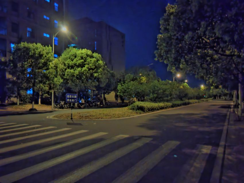
scene illumination [6] where unlike handcrafted features ex-        neutral gray, and its RGB channels are approximately the
plored previously, this CNN model accepted spatial image            same. Since the gray surface presumably reflects all incom-
patches for illumination estimation directly. The CCC [3],          ing light radiation, it can be used to represent the ground
a.k.a., convolutional color constancy, and its follow-up re-        truth illumination of the RAW image accordingly.
finement FFCC [4], a.k.a., Fast fourier color constancy, pro-           We then perform the 2-stage labeling using the illumi-
posed by Barron et al., reformulated the color constancy            nation from the 1-stage. Specifically, first we get the cor-
problem as a 2D spatial localization task in log chromaticity       rect color image by a serial operations including linear de-
space, and thereby applied object detection and structured          mosaicing, white balance using the label white balance and
prediction techniques to solve it.                                  color correction with the camera inner color correction ma-
    Tone mapping operator converts High Dynamic Range               trix (CCM). The brightness adjustment consists of local and
(HDR) image to its Low Dynamic Range (LDR) represen-                global tone mapping jointly. Since local tone mapping re-
tation for the rendering on normal LDR displays. To train           quires fine-grained adjustment of each small patch in the
HDR-LDR mapping, a popular approach was to use a tone-              scene, it is difficult to annotate it manually. Therefore, we
mapping operator (TMO) to generate a set of image labels            use a pre-trained local tone mapping model in [37] to fulfill
and narrow it down using an image quality index to obtain           the task. Since the pre-trained tone mapping network was
final training examples [30, 31]. By incorporating the man-         trained using daytime image, it is good for local adjustment,
ual supervision, Zhang et al. proposed a tone mapping net-          but fails to control the global brightness. We save the model
work (TMNet) in Hue-Saturation-Value (HSV) color space              output using a 16-bit intermediate format in PNG, and then
to obtain better luminance and color mapping results [39].          import it into the Lightroom app to adjust the global expo-
Montulet et al. introduced a new end-to-end tone mapping            sure, brightness, shadows and contrast manually for final
approach based on Deep Convolutional Adversarial Net-               high-quality RGB image rendering, with which we emulate
works (DCGANs) along with a data augmentation tech-                 the image rendering knowledge from Professional Photog-
nique, which reportedly showed the state-of-the-art results         raphers.
on benchmark datasets [27].                                             Thereafter, we successfully obtain a high-resolution
    As a matter of fact, most works mentioned above mainly          nighttime RAW-RGB image dataset for the training of
paid their attention on daytime image optimization. In con-         CBUnet in next sections.
trast, this work deals with the nighttime image rendering by
building a nighttime RAW-RGB dataset and developing a               3.2. CBUnet Architecture
two-stage CBUnet to reconstruct “visually more pleasing”
                                                                        Figure 3 illustrates the architecture of the proposed
images from RAW scenes acquired during the night.
                                                                    CBUnet. It consists of two stages, which are cascaded
                                                                    for color correction and brightness adjustment, respectively.
3. Method                                                           The first stage takes an demosaiced noise free RAW im-
3.1. NR2R Dataset                                                   age Iraw as input. We modified an encoder-decoder based
                                                                    Unet [3] as our primary backbone to estimate the illumi-
   RAW Samples. To form the collection of nighttime                 nation color. The network’s deep features are usually too
RAW samples, we first selected a total of 150 images with           generic without special emphasis even though it is clear
the spatial resolution at 3464×5202 from the training and           that some channel features are more significant than oth-
validation sets provided by the night image challenge [13].         ers in different scenes. In order to make the Unet pay
And then these RAW images are pre-processed to best pro-            more attention to these crucial channels, we employ channel
duce noise-free samples using a notable CNN based de-               attention-convolutions (CA-Convs) blocks inherited from
noiser [1]. This is because nighttime imaging experiences           W-Net [34] to specify the various scenes’ response. As
a very challenging situation with heavy noises incurred by          shown in Figure 4, CA-Convs block first uses global pool-
high ISO setting under poor illumination condition (e.g.,           ing to extract spatial information from convolutional fea-
underexposure).                                                     tures, and then transforms them via fully connected layers
   Paired RGB Derivation. We applied a two-stage pro-               (FC), ReLU, and sigmoid. At last, it multiplies the convo-
cess to derive the corresponding RGB image of each RAW              lutional features with sigmoid’s output, a.k.a., the weights
input.                                                              of the channel attention. All activation functions are imple-
   As shown in Fig. 2, we first used a simple ISP that was          mented with 0.2 negative slope’s parametric rectified lin-
comprised of linear demosaicing, gray-world white balance,          ear units (PReLU) [16]. We apply global average pooling
color correction, and gamma correction to convert each de-          to get the predict illumination color R̂ at the output layer.
noised RAW input to its RGB format for groundtruth illumi-          The input Iraw is then corrected based on the R̂, and the
nation estimation. To this aim, we mark the “White Patch”           color space is further converted to CIE-XYZ based on the
from each converted RGB, where the patch is presented in            in-camera CCM. The whole process of stage 1 can be writ-

                                                                3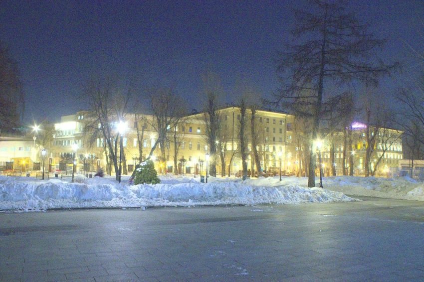
demosaic
bilinear demosaic
demosaic
gamma correction
export 8bits RGB
demosaic
AWB
correction
Label
gray-world
White Balance White Patch
bilinear
bilinear
bilinear
Ground Truth Illumination
color
Denoised RAW White Patch Annotation
Simple ISP
export 16bits RGB
ground truth AWB
NN tone mapping
bilinear demosaic
color correction
Label
Tone Mapping
Denoised RAW NN ISP Lightroom Annotation Expert RGB
Figure 2. Labeling pipeline. We first perform the white balance annotation to derive the ground truth illumination; then input denoised RAW
with estimated ground truth illumination into the NN ISP module (including bilinear demosaic, AWB, color correction, tone mapping) to
obtain the brightness-adjusted RGB image, and finally use Lightroom to adjust global exposure, brightness, shadows and contrasts.
Stage 1 (Color Adjustment)
Demosaic Unet with WB & Color
(Bilinear) Channel Attention Correction
Estimated
Denoised RAW Demosaiced RAW Color CIE-XYZ
Stage 2 (Brightness Adjustment)
Unet with
Convert to Channel Attention Colorize
Grayscale & Hist Branch
Grayscale CIE-XYZ Grayscale RGB Output RGB
Figure 3. The architecture of the CBUnet. It consist of two stages, where the first stage is used to correct the color and the second one
adjusts the brightness for a high-quality output.
ten as: lated as:
Iˆcie-xyz = CCM · f (Iraw ) · Iraw , (1) g G Iˆcie-xyz
Iˆrgb = · Iˆcie-xyz , (2)
G Iˆcie-xyz
where f (·) is the illumination color estimation neural net-
work. where G (·) is the grayscale function.
The second stage is mainly used to adjust the brightness,
so we do not change the color properties of the image at this 4. Experiment
stage. We first extract the grayscale component of Iˆcie-xyz
4.1. Loss Function
and then feed it into the brightness prediction network g (·)
to get the target brightness map, and then colorize it accord- Angular Loss In stage 1, we use angular loss as an
ing to the color information in Iˆcie-xyz . The structure of evaluation criterion between prediction illumination color
the g (·) is similar to the f (·) in stage 1, but an additional R̂ [5, 6] and ground truth illumination R:
histogram extraction branch is added to obtain the global 180
brightness distribution. Histogram extraction branch uses a arccos(R̂ · R).
Langular = (3)
π
256 bits histogram of the Iˆcie-xyz as input, passes through
Pixel Loss In stage 2, we first use L1 Loss to ensure the
two fully connected layers with ReLU activation functions,
accuracy of local tone mapping, which is defined as:
and finally expands to the same size as Unet’s bottom fea-
ture and sums directly. Thus, the stage 2 could be formu- L1 = kG(Iˆrgb ) − G(Irgb )k. (4)
4
Leaky ReLU

                                                                                                                                                               Leaky ReLU

                                                                                                                                                                                       Leaky ReLU
                                                                                                                            Conv 3X3

                                                                                                                                                    Conv 3X3

                                                                                                                                                                            Conv 3X3
                                                                                                                    Convs
               stage 2 only

                                                                                 Conv 3X3        global pooling                              concatenation

                                                                      CA-Convs
                                                                                                      FC
                                                                                                                                             upsampling
                                                                                                     ReLU
                              Histogram                                                                                                      residual connection
                               branch                                                                 FC
                                          stage 2 only                                                                                       downsampling
                                                                            Leaky ReLU             Sigmoid                                   (max pooling)

                              Figure 4. The architecture of our modified Unet. The histogram branch is only used in stage 2.

   Histogram Loss However, it is difficult to constrain the                                  Method                PSNR                         Parameter (M)                                       FLOPs (G)
global brightness distribution by using L1 only, so we use                                   PyNET [21]            20.67                            47.55                                            1370.79
the histogram loss to make the histogram of the generated                                    HERN [26]             19.57                            56.18                                             466.74
images conform to the statistical distribution of the night-                                 AWNet [10]            21.16                            46.99                                            1532.46
time images. The histogram loss could be formulated as:                                      Ours                  22.29                            23.64                                             391.58

               Lhist = kH(Iˆrgb ) − H(Irgb )k,                        (5)                   Table 2. Comparative studies of reconstruction PSNR, parameter
                                                                                            size and FLOPs, where FLOPs is calculated when the input size is
where H is differentiable histogram function from [35].                                     1024 × 1024.
   Finally, we define our loss function by the sum of the
aforementioned losses as follows:                                                                    CA           Two Stage                         Hist Branch                                     PSNR
                                                                                                                                                                                                    19.85
             Ltotal = Langular + L1 + Lhist .                         (6)                             √
                                                                                                                                                                                                    20.53
                                                                                                      √                     √
4.2. Training Details                                                                                                                                                                               22.01
                                                                                                      √                     √                                  √
                                                                                                                                                                                                    22.29
   The model was implemented in Pytorch and was trained
on a single Nvidia Tesla 3090 GPU with a batch size                                         Table 3. Ablation studies on network architectures, where CA and
16. We devide the NR2R dataset into two parts: 120 im-                                      Hist Branch mean channel attention and histogram branch, respec-
ages are used for training and the rest 30 images are used                                  tively.
for testing. The stage 1 was first pretrained on Cube++
dataset [12] which is captured within the same camera of the
NR2R.Then we use Adam optimizer [23] with 5e-5 learn-                                       only present a very small fraction percentage (e.g.,
(a) RAW (visulized)                   (b) PyNET (PSNR: 17.25dB)                (c) HERN (PSNR: 19.42dB)

           (d) AWNet (PSNR: 17.09dB)                     (e) Ours (PSNR: 20.39dB)                   (f) Ground Truth

Figure 5. Visual comparison of reconstructions from four different methods including PyNET [21], HERN [26], AWNet [10] and our
proposed CBUnet.

             L1     Langular     Lhist     PSNR                         but the NR2R dataset was captured by a single DSLR cam-
             √
                                           21.98                        era. Thus, we test our method on a mobile phone camera
             √         √
                                           22.14                        to verify the generalization of our method. We took a set
             √         √           √
                                           22.29                        of nighttime RAW images with a resolution of 4032 × 3024
                                                                        using the main camera of iPhone 8 Plus which has a com-
          Table 4. Ablation studies on loss functions.                  pletely different CMOS and optical lens. Figure 6 shows
                                                                        that our CBUnet has better color correction compared to
                                                                        the iPhone’s internal ISP, e.g. zebra lines are correctly cor-
   Loss Function Then, we verified the efficiency of our                rected to white and the sky is blue. Also, our model renders
loss function which consists of pixel loss L1 , angular loss            images with better retention of details in the shadow and
Langular and histogram loss Lhist . The experimental re-                better suppression of highlights such as haloes.
sults are shown in Table 4. When Langular is added, 0.16
dB PSNR increase was achieved. Finally, the addition of                 4.6. NTIRE 2022 Night Photography Rendering
Lhist also improved the results in a gain of 0.15 dB.                        Challenge

4.5. Generalization to Other Camera Sensors                                As for the NTIRE 2022 Night Photography Rendering
                                                                        Challenge [13], We submitted 100 night images rendered
   Although our proposed CBUnet achieved the best per-                  with this method. Rendering results are shown in Figure 7.
formance with minimal computation in the NR2R dataset,                  The baseline ISP provided by challenge organizers consists

                                                                    6
RAW (visualized)                     iPhone 8 Plus ISP                              Ours
Figure 6. The results of the proposed CBUnet on RAW images from the iPhone 8 Plus smartphone. From left to right: the original
visualized RAW image, the same photo obtained with iPhone’s built-in ISP system and our reconstructed RGB image.

               RAW(visualized)                           Baseline                                   Ours
               Figure 7. Rendering Results of our CBUnet in the NITRE 2022 Photography Rendering Challenge [13].

of bilinear demosaicing, bilateral denosing, AWB using            gray world assumption, color space conversion with cam-

                                                              7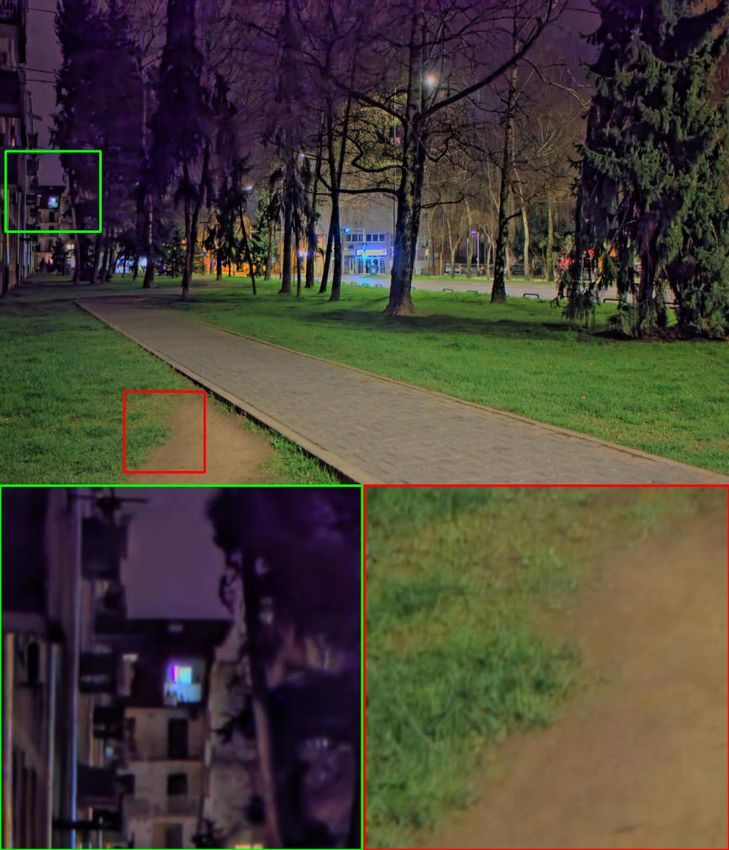
era inner CCM and flash tone mapping [2]. Compared to                        ropean Conference on Computer Vision, pages 185–201.
the baseline ISP, our renderings have a more accurate white                  Springer, 2020. 5, 6
balance and a brightness distribution that is more consistent         [11]   Eric Dubois. Filter design for adaptive frequency-domain
with nighttime scene characteristics.                                        bayer demosaicking. In 2006 International Conference on
                                                                             Image Processing, pages 2705–2708. IEEE, 2006. 2
5. Conclusion                                                         [12]   Egor Ershov, Alexey Savchik, Illya Semenkov, Nikola Banić,
                                                                             Alexander Belokopytov, Daria Senshina, Karlo Koščević,
    Night photography is challenging due to the lack of suf-                 Marko Subašić, and Sven Lončarić. The cube++ illumination
ficient nighttime image dataset and comprehensive under-                     estimation dataset. IEEE Access, 8:227511–227527, 2020. 5
standing of complex light illumination in the night. This             [13]   Egor Ershov, Alex Savchik, Denis Shepelev, Nikola Banic,
work therefore built a NR2R dataset with dedicated expert                    Michael S Brown, Radu Timofte, et al. NTIRE 2022 chal-
annotations as the ground-truth for NN ISP training, and                     lenge on night photography rendering. In Proceedings of
                                                                             the IEEE/CVF Conference on Computer Vision and Pattern
developed a CBUnet for rendering image in the night. The
                                                                             Recognition (CVPR) Workshops, 2022. 1, 2, 3, 6, 7
proposed CBUnet showed high-performance and consis-
                                                                      [14]   Alessandro Foi, Mejdi Trimeche, Vladimir Katkovnik, and
tent imaging capacity voted by both experts and amateurs,                    Karen Egiazarian. Practical poissonian-gaussian noise mod-
reporting the second place in the NTIRE 2022 Night Pho-                      eling and fitting for single-image raw-data. IEEE Transac-
tography Rendering Challenge for both People’s and Pho-                      tions on Image Processing, 17(10):1737–1754, 2008. 2
tographer’s choices.                                                  [15]   Arjan Gijsenij, Theo Gevers, and Joost Van De Weijer. Im-
                                                                             proving color constancy by photometric edge weighting.
References                                                                   IEEE Transactions on Pattern Analysis and Machine Intel-
                                                                             ligence, 34(5):918–929, 2011. 2
 [1] Abdelrahman Abdelhamed, Mahmoud Afifi, Radu Timofte,
                                                                      [16]   Kaiming He, Xiangyu Zhang, Shaoqing Ren, and Jian Sun.
     and Michael S Brown. Ntire 2020 challenge on real image
                                                                             Delving deep into rectifiers: Surpassing human-level perfor-
     denoising: Dataset, methods and results. In Proceedings of
                                                                             mance on imagenet classification. In Proceedings of the
     the IEEE/CVF Conference on Computer Vision and Pattern
                                                                             IEEE international conference on computer vision, pages
     Recognition Workshops, pages 496–497, 2020. 3
                                                                             1026–1034, 2015. 3
 [2] Nikola Banic and Sven Loncaric. Flash and storm: Fast and        [17]   Keigo Hirakawa and Thomas W Parks.                   Adaptive
     highly practical tone mapping based on naka-rushton equa-               homogeneity-directed demosaicing algorithm. Ieee transac-
     tion. In VISIGRAPP (4: VISAPP), pages 47–53, 2018. 8                    tions on image processing, 14(3):360–369, 2005. 2
 [3] Jonathan T Barron. Convolutional color constancy. In Pro-        [18]   Jie Huang, Pengfei Zhu, Mingrui Geng, Jiewen Ran, Xing-
     ceedings of the IEEE International Conference on Computer               guang Zhou, Chen Xing, Pengfei Wan, and Xiangyang Ji.
     Vision, pages 379–387, 2015. 3                                          Range scaling global u-net for perceptual image enhance-
 [4] Jonathan T Barron and Yun-Ta Tsai. Fast fourier color con-              ment on mobile devices. In Proceedings of the European
     stancy. In Proceedings of the IEEE conference on computer               conference on computer vision (ECCV) workshops, pages 0–
     vision and pattern recognition, pages 886–894, 2017. 3                  0, 2018. 2
 [5] Simone Bianco and Claudio Cusano. Quasi-unsupervised             [19]   Zheng Hui, Xiumei Wang, Lirui Deng, and Xinbo Gao.
     color constancy. In Proceedings of the IEEE/CVF Confer-                 Perception-preserving convolutional networks for image en-
     ence on Computer Vision and Pattern Recognition, pages                  hancement on smartphones. In Proceedings of the European
     12212–12221, 2019. 1, 4                                                 Conference on Computer Vision (ECCV) Workshops, pages
 [6] Simone Bianco, Claudio Cusano, and Raimondo Schettini.                  0–0, 2018. 2
     Single and multiple illuminant estimation using convolu-         [20]   Andrey Ignatov, Luc Van Gool, and Radu Timofte. Replac-
     tional neural networks. IEEE Transactions on Image Pro-                 ing mobile camera isp with a single deep learning model.
     cessing, 26(9):4347–4362, 2017. 1, 3, 4                                 In Proceedings of the IEEE/CVF Conference on Computer
 [7] Antoni Buades, Bartomeu Coll, and J-M Morel. A non-local                Vision and Pattern Recognition Workshops, pages 536–537,
     algorithm for image denoising. In 2005 IEEE Computer So-                2020. 2
     ciety Conference on Computer Vision and Pattern Recogni-         [21]   Andrey Ignatov, Luc Van Gool, and Radu Timofte. Replac-
     tion (CVPR’05), volume 2, pages 60–65. IEEE, 2005. 2                    ing mobile camera isp with a single deep learning model.
 [8] Gershon Buchsbaum. A spatial processor model for ob-                    In Proceedings of the IEEE/CVF Conference on Computer
     ject colour perception. Journal of the Franklin institute,              Vision and Pattern Recognition Workshops, pages 536–537,
     310(1):1–26, 1980. 2                                                    2020. 5, 6
 [9] Laurent Condat. A simple, fast and efficient approach to         [22]   Nima Khademi Kalantari, Ravi Ramamoorthi, et al. Deep
     denoisaicking: Joint demosaicking and denoising. In 2010                high dynamic range imaging of dynamic scenes. ACM Trans.
     IEEE International Conference on Image Processing, pages                Graph., 36(4):144–1, 2017. 2
     905–908. IEEE, 2010. 2                                           [23]   Diederik P Kingma and Jimmy Ba. Adam: A method for
[10] Linhui Dai, Xiaohong Liu, Chengqi Li, and Jun Chen.                     stochastic optimization. arXiv preprint arXiv:1412.6980,
     Awnet: Attentive wavelet network for image isp. In Eu-                  2014. 5

                                                                  8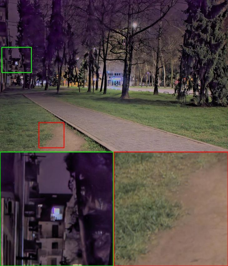
[24] Xin Li, Bahadir Gunturk, and Lei Zhang. Image demosaic-            [38] Akiko Yoshida, Volker Blanz, Karol Myszkowski, and Hans-
     ing: A systematic survey. In Visual Communications and                  Peter Seidel. Perceptual evaluation of tone mapping opera-
     Image Processing 2008, volume 6822, pages 489–503. SPIE,                tors with real-world scenes. In Human Vision and Electronic
     2008. 2                                                                 Imaging X, volume 5666, pages 192–203. International So-
[25] Laurence T Maloney. Physics-based approaches to model-                  ciety for Optics and Photonics, 2005. 1
     ing surface color perception. Color vision: From genes to          [39] Ning Zhang, Chao Wang, Yang Zhao, and Ronggang Wang.
     perception, pages 387–416, 1999. 1                                      Deep tone mapping network in hsv color space. In 2019
[26] Kangfu Mei, Juncheng Li, Jiajie Zhang, Haoyu Wu, Jie Li,                IEEE Visual Communications and Image Processing (VCIP),
     and Rui Huang. Higher-resolution network for image de-                  pages 1–4. IEEE, 2019. 3
     mosaicing and enhancing. In 2019 IEEE/CVF International            [40] Xin Zhang and Ruiyuan Wu. Fast depth image denoising
     Conference on Computer Vision Workshop (ICCVW), pages                   and enhancement using a deep convolutional network. In
     3441–3448. IEEE, 2019. 5, 6                                             2016 IEEE International Conference on Acoustics, Speech
[27] Rico Montulet, Alexia Briassouli, and N Maastricht. Deep                and Signal Processing (ICASSP), pages 2499–2503, 2016. 2
     learning for robust end-to-end tone mapping. In BMVC, vol-         [41] Erjin Zhou, Haoqiang Fan, Zhimin Cao, Yuning Jiang, and
     ume 2, page 4, 2019. 3                                                  Qi Yin. Learning face hallucination in the wild. In Twenty-
                                                                             ninth AAAI conference on artificial intelligence, 2015. 2
[28] Karen Panetta, Landry Kezebou, Victor Oludare, Sos Aga-
     ian, and Zehua Xia. Tmo-net: A parameter-free tone map-
     ping operator using generative adversarial network, and per-
     formance benchmarking on large scale hdr dataset. IEEE
     Access, 9:39500–39517, 2021. 1
[29] Bumjun Park and Jechang Jeong. Color filter array demo-
     saicking using densely connected residual network. IEEE
     Access, 7:128076–128085, 2019. 2
[30] Vaibhav Amit Patel, Purvik Shah, and Shanmuganathan Ra-
     man. A generative adversarial network for tone mapping hdr
     images. In National Conference on Computer Vision, Pattern
     Recognition, Image Processing, and Graphics, pages 220–
     231. Springer, 2017. 3
[31] Aakanksha Rana, Praveer Singh, Giuseppe Valenzise, Fred-
     eric Dufaux, Nikos Komodakis, and Aljosa Smolic. Deep
     tone mapping operator for high dynamic range images. IEEE
     Transactions on Image Processing, 29:1285–1298, 2019. 3
[32] Olaf Ronneberger, Philipp Fischer, and Thomas Brox. U-
     net: Convolutional networks for biomedical image segmen-
     tation. In International Conference on Medical image com-
     puting and computer-assisted intervention, pages 234–241.
     Springer, 2015. 2
[33] Jack Tumblin and Holly Rushmeier. Tone reproduction for
     realistic images. IEEE Computer graphics and Applications,
     13(6):42–48, 1993. 2
[34] Kwang-Hyun Uhm, Seung-Wook Kim, Seo-Won Ji, Sung-
     Jin Cho, Jun-Pyo Hong, and Sung-Jea Ko. W-net: Two-
     stage u-net with misaligned data for raw-to-rgb mapping. In
     2019 IEEE/CVF International Conference on Computer Vi-
     sion Workshop (ICCVW), pages 3636–3642. IEEE, 2019. 3
[35] Evgeniya Ustinova and Victor Lempitsky. Learning deep
     embeddings with histogram loss. Advances in Neural In-
     formation Processing Systems, 29, 2016. 5
[36] Joost Van De Weijer, Theo Gevers, and Arjan Gijsenij. Edge-
     based color constancy. IEEE Transactions on image process-
     ing, 16(9):2207–2214, 2007. 2
[37] Yael Vinker, Inbar Huberman-Spiegelglas, and Raanan Fat-
     tal. Unpaired learning for high dynamic range image tone
     mapping. In Proceedings of the IEEE/CVF International
     Conference on Computer Vision, pages 14657–14666, 2021.
     3

                                                                    9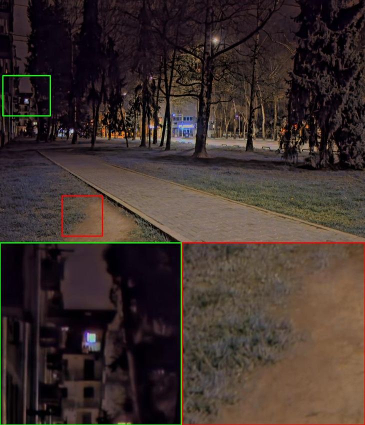
You can also read