RED PANDA: DISAMBIGUATING IMAGE ANOMALY DE- TECTION BY REMOVING NUISANCE FACTORS
←
→
Page content transcription
If your browser does not render page correctly, please read the page content below
Published as a conference paper at ICLR 2023

R ED PANDA: D ISAMBIGUATING I MAGE A NOMALY D E -
TECTION BY R EMOVING N UISANCE FACTORS

 Niv Cohen     Jonathan Kahana           Yedid Hoshen
 School of Computer Science and Engineering
 The Hebrew University of Jerusalem, Israel
 nivc@cs.huji.ac.il

                                                A BSTRACT

             Anomaly detection methods strive to discover patterns that differ from the norm
             in a meaningful way. This goal is ambiguous as different human operators may
             find different attributes meaningful. An image differing from the norm by an
             attribute such as pose may be considered anomalous by some operators while
             others may consider the attribute irrelevant. Breaking from previous research,
             we present a new anomaly detection method that allows operators to exclude an
             attribute when detecting anomalies. Our approach aims to learn representations
             which do not contain information regarding such nuisance attributes. Anomaly
             scoring is performed using a density-based approach. Importantly, our approach
             does not require specifying the attributes where anomalies could appear, which
             is typically impossible in anomaly detection, but only attributes to ignore. An
             empirical investigation is presented verifying the effectiveness of our approach1 .

1       I NTRODUCTION

Anomaly detection, discovering unusual patterns in data, is a key capability for many machine
learning and computer vision applications. In the typical setting, the learner is provided with training
data consisting only of normal samples, and is then tasked with classifying new samples as normal or
anomalous. It has emerged that the representations used to describe data are key for anomaly detection
in images and videos (Reiss et al., 2021). Advances in deep representation learning (Huh et al.,
2016) have been used to significantly boost anomaly detection performance on standard benchmarks.
However, these methods have not specifically addressed biases in the used data. Anomaly detection
methods which suffer from the existence of such biases may produce more overall errors, and
incorrectly classify as anomalies some types of samples more than others. A major source for such
biases is the presence of additional, nuisance factors (Lee & Wang, 2020).
One of the most important and unsolved challenges of anomaly detection is resolving the ambiguity
between relevant and nuisance attributes. As a motivating example let us consider the application
of detecting unusual vehicles using road cameras. Normal samples consist of images of known
vehicle types. When aiming to detect anomalies, we may encounter two kinds of difficulties: (i) The
distribution of unknown vehicles (anomalies) is not known at training time. E.g., unexpected traffic
may come in many forms: a horse cart, heavy construction equipment, or even wild animals. This is
the standard problem addressed by most anomaly detection methods (Ruff et al., 2018; Reiss et al.,
2021; Tack et al., 2020). (ii) The normal data may be biased. For example, assume all agricultural
machinery appearing during the collection of normal data was moved towards the farmlands. During
inference performed on another season, we may see the same equipment moving to the other side
(and from a different angle). This novel view might be incorrectly perceived as an anomaly.
Unlike previous works, we aim to disambiguate between true anomalies (e.g., unseen vehicle types)
and unusual variations of nuisance attributes in normal data (e.g., a known vehicle observed previously
only in another direction). Detecting normal but unusual variations according to nuisance attributes
as anomalies may be a source of false positive alarms. In addition, they may introduce an undesirable
imbalance in the detected anomalies, or even discriminate against certain groups. There are many
    1
        The presented benchmarks are available on github under: https://github.com/NivC/RedPANDA.

                                                      1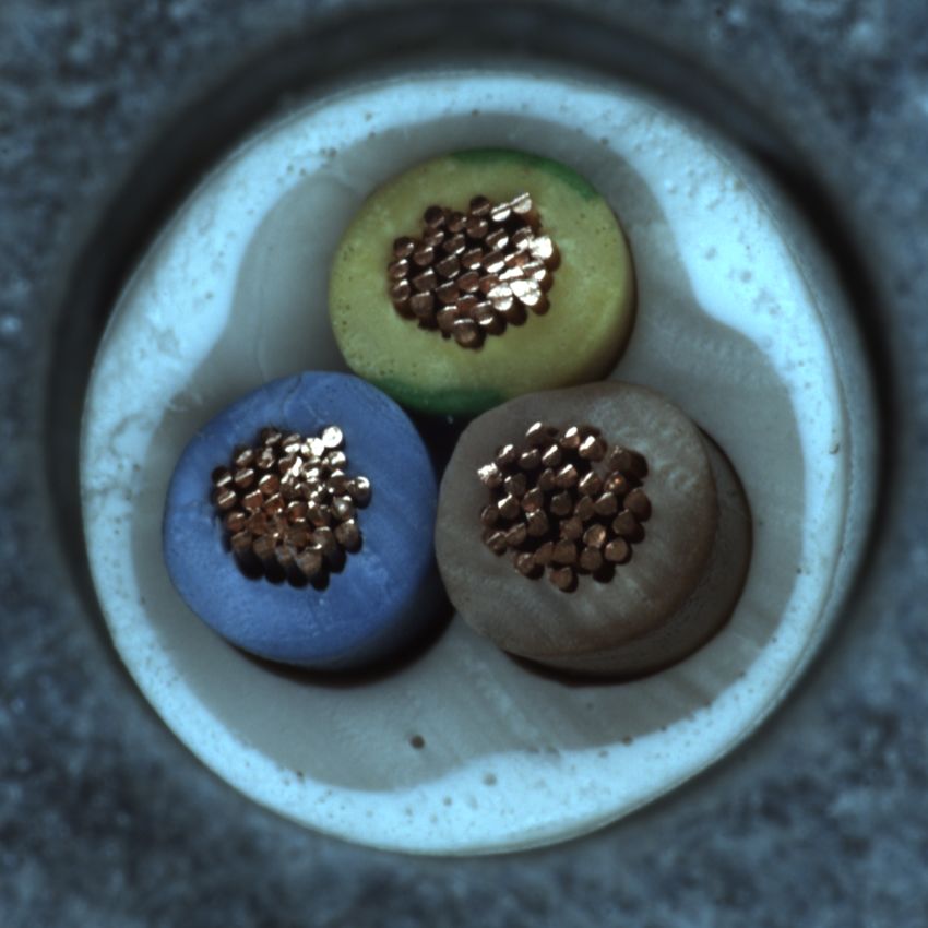
Published as a conference paper at ICLR 2023

settings where some attribute combinations are missing from the training dataset but are considered
normal: assembly line training images may be biased in terms of lighting conditions or camera angles
- while these may be irrelevant to their anomaly score; photos of people may be biased in terms
of ethnicity, for example when collected in specific geographical areas. Moreover, in some cases,
normal attribute combinations may be absent just due to the rarity of some attributes (e.g. rare car
colors with specific car models).
The task of learning to ignore nuisance attributes requires a general approach. While simple heuristics
might sometimes be possible, they suffer from inherent weaknesses: (i) lack of generalization to new
image types and nuisance attributes (ii) targeting a specific type of anomalies, which means they will
fail to generalize to new, unexpected anomalies. While nuisance attribute removal is easy when the
representation is already disentangled in nuisance and relevant components (e.g., some tabular data
settings), most image representations and highly entangled.
Our technical approach proposes to ignore nuisance attributes by learning representations that are
independent from them. Our approach takes as input a training set of normal samples with a labeled
nuisance attribute. We utilize a domain-supervised disentanglement approach (Kahana & Hoshen,
2022) to remove the information associated with the provided nuisance attribute, while preserving
as much uncorrelated information as possible about the image. Specifically, we train an encoder
with an additional per-domain contrastive loss term to learn a representation which is independent
of the labeled nuisance attribute. For example, an encoder guided to be invariant to the viewing
angle would be trained to contrast images of cars driving to the left with similar images, but not
against images of cars driving to the right. Additionally, a conditional generator is trained on the
representations with a reconstruction term, to ensure the representations are informative. We stress
that we only use the reconstruction loss to encourage the informativeness of our encoder, and do
not use the reconstruction errors to score anomalies. The combination of the two loss terms yields
informative representations which are less sensitive to the nuisance attributes. Although our obtained
representation is far from being completely invariant to the nuisance attributes, it provides significant
gains on several benchmarks. The representations are then combined with standard density estimation
methods (k nearest neighbors) for anomaly scoring.
Our setting differs from previous ones, as it only relies on nuisance attribute labels. Few anomaly
detection algorithms consider the case where the training set contains attribute labels and therefore
most methods do not aim to ignore nuisance attributes. Out-of-distribution detection assumes that
normal data are labelled with the value of the relevant attribute and that anomalies belong to a novel
class, outside the set of labelled values (Salehi et al., 2021; Hendrycks et al., 2020; Hendrycks &
Gimpel, 2016). The weakly supervised setting assumes future anomalies will be similar to a few
labelled anomalous samples available during training (Cozzolino et al., 2018; Gianchandani et al.,
2019; Deecke et al., 2021). However, this type of knowledge is often limiting due to the inherent
unpredictability of anomalies. In contrast, we only require knowledge of the factors that are not
indicative of the anomalies we wish to find - while assuming no specific knowledge of the expected
anomalies. In fact, labels for attributes we wish to ignore are often provided by the datasets, such as
information about the sensor used to collect the data. In other cases, such labels are easily predicted
using pre-trained classifiers such as CLIP (Radford et al., 2021).
As this task is novel, we present new benchmarks and new metrics for evaluation. Our benchmarks
incorporate normal examples which experience unusual variation in a nuisance attribute. Our
evaluation metrics measure both the overall anomaly detection accuracy, as well as the false alarm
rate due to mistaking normal samples with nuisance variation as anomalies. Our experiments indicate
that using our approach for removing the dependencies on a nuisance attribute from the representation
improves these metrics on our evaluation datasets. While our method can currently handle only quite
simple cases, this study indicates a way forward for tackling more realistic cases.
Contributions: (i) Introducing the novel setting of Negative Attribute Guided Anomaly Detection
(NAGAD). (ii) Presenting new evaluation benchmarks and metrics for the NAGAD setting (iii)
Proposing a new approach, REpresentation Disentanglement for Pre-trained Anomaly Detection
Adaptation (Red PANDA), using domain-supervised disentanglement to address this setting. (iv)
Demonstrating the potential of our approach through empirical evaluation.

                                                   2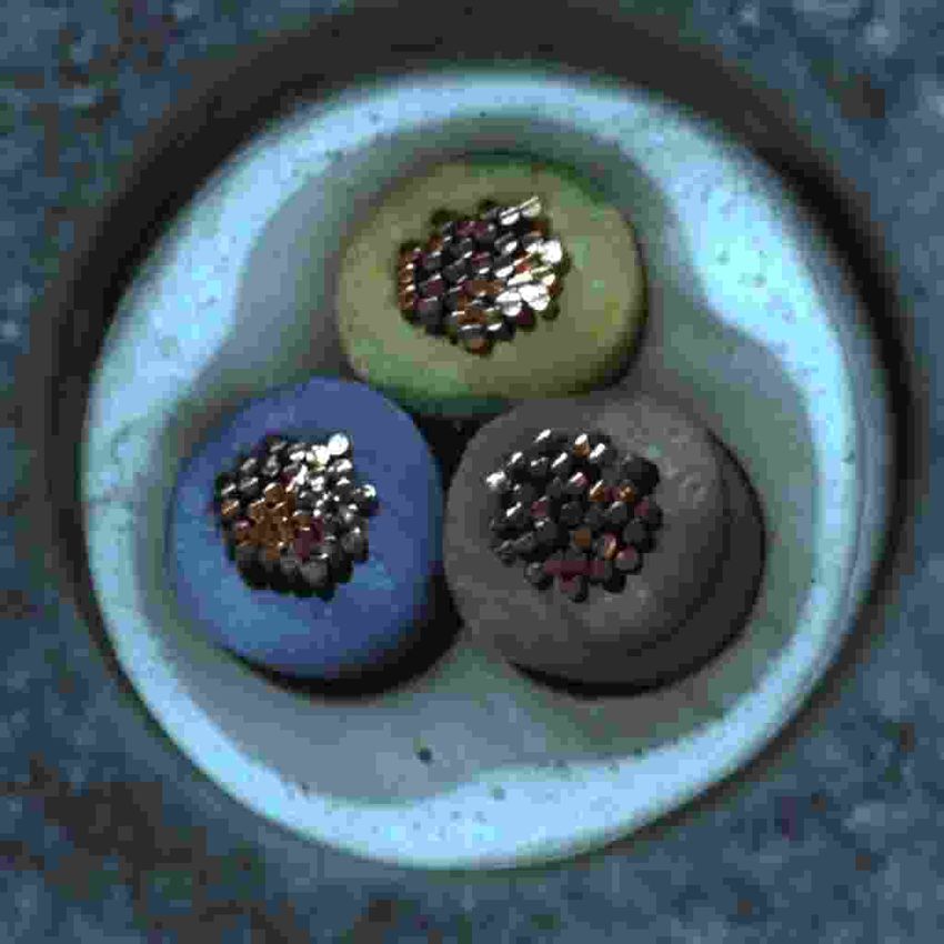
Published as a conference paper at ICLR 2023

2    R ELATED W ORKS

Classical anomaly detection methods. These may be grouped into three themes (Yang et al., 2021;
Ruff et al., 2021): (i) Density-estimation based methods. Estimation of the density of the normal data
can be non-parametric methods, such as kNN or kernel density estimation. Parametric methods, such
as Gaussian Mixture Models (GMM) (Li et al., 2016) learn a parametric representation of the data to
estimate the probability density of the test samples. (ii) Reconstruction-based methods - methods
such as PCA learn to reconstruct well normal training samples. Anomalies coming from a different
distribution might not reconstruct as well. (iii) One class classification methods - A classification
approach separating the normal samples and the rest of feature space (e.g. SVDD (Tax & Duin,
2004)).
Deep anomaly detection methods. As only normal samples are available during training, we cannot
learn features with standard supervision. Therefore, deep anomaly detection methods either use
self-supervision learning to score the anomalies (Hendrycks et al., 2019), or adapt a pre-trained
representation (Hendrycks et al., 2019; Reiss et al., 2021; Reiss & Hoshen, 2021; Ruff et al., 2018;
Perera & Patel, 2019) to describe the normal training data. (i) Self-supervised methods - these methods
learn to solve an auxiliary task on the normal samples, test the performance on new images, and score
anomalies accordingly: the network is expected to perform better on the normal samples that come
from a similar distribution (Hendrycks et al., 2019). More recent works such as CSI (Tack et al., 2020)
or DROC (Goyal et al., 2020) use contrastive learning to learn a representation of the normal data.
(ii) Adaptation of Pre-trained Feature - Transfer learning of pre-trained features was shown to give
strong results for out-of-distribution detection by (Hendrycks et al., 2019). Adaptation of pre-trained
features for anomaly detection was attempted by Deep-SVDD (Ruff et al., 2018), which adapted
features learnt by an auto-encoder using compactness loss. Perera & Patel suggested to training the
compactness loss jointly with ImageNet classification (Perera & Patel, 2019). By incorporating early
stopping and EWC regularization (Kirkpatrick et al., 2017), PANDA (Reiss et al., 2021) allowed
feature adaptation with mitigated catastrophic forgetting, resulting in better performance. Further
improvement in pre-trained feature adaptation was later suggested by MeanShifted (Reiss & Hoshen,
2021), using contrastive learning to adapt the pre-trained features to the normal training set.
Domain-supervised disentanglement. Disentanglement is the process of recovering the latent
factors that are responsible for the variation between samples in a given dataset. For example, from
images of human faces we may recover the age of each person, their hair color, eye color, etc. In
domain-supervised disentanglement, one assumes that a single such factor is labelled and aims to learn
a representation of the other attributes independent of the labelled factor. This task was approached
with variational auto-encoders (Jha et al., 2018; Bouchacourt et al., 2018), and latent optimization
(Gabbay & Hoshen, 2019; 2021). Contrastive methods have also shown great promise with general
disentanglement (Zimmermann et al., 2021). This was followed by Kahana & Hoshen in domain-
supervised disentanglement (Kahana & Hoshen, 2022) who employed a contrastive loss for each
set of similarly-labelled samples individually, learning a code which ideally describes only (and all)
attributes which are uncorrelated to the labelled attributes. Domain-supervised disentanglement has
been used for a variety of applications. Most notably, for generative models (Zhu et al., 2018)(Gabbay
& Hoshen, 2019). Disentanglement models have also been discussed in the context of interpretability
(Hsu et al., 2017), abstract reasoning (Van Steenkiste et al., 2019), domain adaptation (Peng et al.,
2019), and fairness (Creager et al., 2019). Some previous works have considered using domain
supervision for increasing fairness in anomaly detection (Davidson & Ravi, 2020; Zhang & Davidson,
2021; Shekhar et al., 2021). These methods aim at obtaining equal anomaly detection performance
across the protected attributes. On the other hand, our objective is to ignore the nuisance attributes in
order to improve the overall performance of the anomaly detection method.

3    N UISANCE ATTRIBUTES M ISLEAD A NOMALY D ETECTORS

Anomaly detection methods aim to detect samples deviating from the norm. However, operators of
anomaly detection methods expect the deviation to be semantically relevant. As the anomaly detection
setting is typically unsupervised and the type of anomalies cannot be expected, it is impossible to
predict in which modes of variations anomalies will appear. Yet, we may know in advance that
we do not wish to detect anomalies in nuisance attributes. For example, we may wish to detect
anomalous vehicles in traffic. Anomalies can appear in many attributes such as car type, color,

                                                   3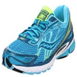
Published as a conference paper at ICLR 2023

condition, headlights type, etc. However, if we do not wish to detect anomalies in the car pose,
avoiding false positives associated with this attribute may be possible without knowing in advance in
which attributes anomalies will appear.
Current algorithms rely on different inductive biases to select the relevant attributes and remove the
nuisance ones. The most common choice is manual feature selection, where the operator specifies
particular features that would be the most relevant (Pevnỳ, 2016; Gu et al., 2019). Contrastive
learning methods specify augmentations which remove specific attributes (minor color and location
variations) from the representation. This helps to select attributes more relevant to object-centric
tasks. Similarly, representations pre-trained on supervised object classification (e.g. ImageNet (Deng
et al., 2009)), which have recently demonstrated very strong results on image anomaly detection,
focus on object-centric attributes at the expense of other low-level image attributes. The most extreme
level of supervision is the out-of-distribution detection setting, where the class labels are provided
for all normal training data, and anomalies are expected to belong to an unseen class. However, this
guidance is not available in the typical anomaly detection setting as anomalies are unexpected.
Our novel setting, Negative Attribute Guided Anomaly Detection (NAGAD), allows the specification
of nuisance attributes that should be ignored by the anomaly detector. Unlike specifying the relevant
attributes, which is not possible in anomaly detection, specifying nuisance attributes is often possible.
Users may know in advance about the attributes they wish to exclude for anomaly detection; either
due to legal and moral reasons, or due to prior domain knowledge. The issue of excluding such
attributes from images remains a major technical challenge even when such attributes are known.
A natural way for specifying nuisance attributes is to provide labels for them. For example, wishing
to detect anomalies according to a car model but not according to its pose, we may provide for each
image a label for the car pose (see Fig.1). Currently available anomaly detection approaches cannot
directly benefit from such information and thus mitigate nuisance attributes only implicitly (using
the mechanisms explained above). In Sec. 4 we describe a specific technical approach for using
the guidance for anomaly detection. Yet, we stress that our main contribution is the novel anomaly
detection setting.

4     R ED PANDA: D ISENTANGLEMENT A PPROACH FOR R EMOVING A
      N UISANCE FACTOR

We detail the different stages of our approach below. An algorithm box summarizing the different
steps can be found in App.J.

4.1   O BTAINING L ABELS FOR THE N UISANCE ATTRIBUTE

Our approach, REpresentation Disentanglement for Pre-trained Anomaly Detection Adaptation (Red
PANDA), aims to achieve a representation invariant to a nuisance attribute of our dataset, leading
to better detection of anomalies expressed in relevant attributes. To do so, we provide labels for the
nuisance attribute. For example, when we wish to detect anomalies in driver behaviour, we may wish
to ignore the vehicle’s pose. We can achieve this by providing pose labels during training, and using
them to be less sensitive to this attribute.
To achieve these labels, we have a few options. In some cases, they may already exist in the dataset.
A very natural such case is when we have data from a few static cameras, and we wish to ignore
the camera identity. In many other cases, a pre-trained classifier, already trained for these specific
attributes may provide such labels. Recently, pre-trained models for text-based zero-shot classification
such as CLIP (Radford et al., 2021) have shown promising results. Such models allow supplying
of-the-shelf labels for a very large set of attributes. We conducted a small experiment over the
Edges2Shoes (Isola et al., 2017) dataset, automatically labelling it with CLIP, and achieved 99.97%
accuracy in labelling whether an image is a photo or a sketch (Fig.2). Taken together in many cases
labels for nuisance attributes can be achieved at virtually no cost.

                                                   4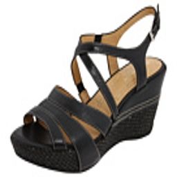
Published as a conference paper at ICLR 2023

4.2   P RELIMINARIES

In our setting, the training set denoted as Dtrain consists of normal samples only . For each normal
image xi ∈ Dtrain we are also provided with its label ni describing the nuisance attribute we
wish to ignore (the setting can be naturally extended to many nuisance attributes). Our evaluation
set Dtest consists of both normal and anomalous samples. We denote the normal/anomaly label
for a test image xi as yi . For each such dataset, each sample is described by multiple attributes
(ni , ai , bi , ci , ...) ∈ N × A × B × C × ..., where N describe our nuisance attribute, and A, B, C, ...
describe different relevant attributes (consider for example the identity of the object, the lightning
condition, and camera angles as different attributes). We only assume labels for N during training.
We assume that the anomaly label is always a function of (potentially) all the relevant attributes
yi = fa (ai , bi , ci , ...). Namely, we assume the nuisance attribute ni never affects the anomaly label
yi . We emphasize that in our described setting, none of the relevant attribute labels nor the anomaly
labels are given during training.
We aim to learn an encoder function f mapping samples xi to a code describing their relevant
attributes f (xi ) ∈ Rd . We also wish our codes to be invariant. This is, we wish our encoder to
represent the relevant attributes in a way that is not affected by the nuisance attributes:

                                            p(ni ) = p(ni |f (x))                                     (1)

We also wish our code to be informative - to represent sufficient information regarding our relevant
attributes (I(; ) is the mutual information between its two arguments):


                           I (ai , bi , ci , ...); xi ≈ I (ai , bi , ci , ...); f (xi )               (2)

In practice, the invariance may be measured by the accuracy of predicting ni from the latent code
f (x). Similarly, we can measure the accuracy of predicting the relevant attribute used to define
anomalies (informativeness). Empirical evaluations of these measures for our datasets can be found in
the App.I. Given such a representation we may later score anomalies independently from any biases
caused by the nuisance attribute we wish to ignore.

4.3   C ONTRASTIVE D ISENTANGLEMENT

In this section, we describe the technical approach we employ for ensuring that f does not contain
information on the nuisance attribute, while retaining as much information about the relevant attributes
(Kahana & Hoshen, 2022).
Pre-trained encoder. We initialize the encoder function f with an ImageNet pre-trained network.
ImageNet-pre-trained representations were previously shown to be very effective for image anomaly
detection (Reiss et al., 2021). Off-the-self pre-trained representation, however, also encodes much
information on the nuisance attributes. Therefore they do not satisfy our invariance objective.
Contrastive loss. Our objective is that images that have similar relevant attributes but different
nuisance attributes would have similar representations. Although we are not provided with supervised
matching pairs, we use the proxy objective requiring the distribution of representations of images
having different nuisance attributes to be the same. To match the distributions we first split our
training data Dtrain to disjoint subsets Sni according to the nuisance attribute values:

                                                              [
                                             Dtrain =         · Sni                                   (3)
                                                           ni ∈N

We then use a contrastive loss on each of the sets Sni independently (sim denotes cosine similarity,
xi , xj ∈ Dtrain are arbitrary normal samples, and n(xi ), n(xj ) are their nuisance labels):


                                                   1n(xi )=n(xj ) e
                                          X                           sim (f (xi ),f (xj )
                           Lcon = log                                                                 (4)
                                          xi ,xj

                                                          5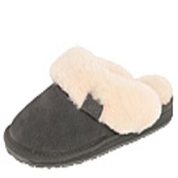
Published as a conference paper at ICLR 2023

This objective encourages the encoder to map the image distribution of each nuisance attribute
uniformly to the unit sphere (Wang & Isola, 2020). Therefore, it matches the distributions of sample
embeddings coming from different values of the nuisance attribute (as required by Eq.1) (Wang
& Isola, 2020). We note that matching of marginal distributions is necessary, but not a sufficient
condition for alignment ((Kahana & Hoshen, 2022)).
Another problem that may arise is insufficient informativeness: the contrastive objective does not
prevent ignoring some of the relevant attributes (Chen et al., 2021). To support the informativeness
we add an augmentation loss, encouraging
                                           different augmentations of the same image to be mapped

to similar codes: Laug = −sim f A1 (xi ), A2 (xi ) . The used augmentations are detailed in
appendix D. To further encourage informativeness, we also employ a reconstruction loss.
Reconstruction loss. To encourage the representation to contain as much information about the
relevant attributes as possible, we use a reconstruction constraint. Specifically, we require that
given the combination of the representation fi (which ideally ignores the nuisance attribute) and the
value of the nuisance attribute ni , it should be possible to perfectly recover the sample xi . This is
enforced using a generator function G which is trained end-to-end together with the encoder. The
reconstruction is measured using a perceptual loss.

                                      X
                           Lrec =               ℓperceptual xi , G f (xi ), ni                        (5)
                                    Dtrain ,N

4.4   D ENSITY BASED A NOMALY S CORING

Similarly to other anomaly detection methods, we hypothesize the anomalous samples will be
mapped to low-density regions, while normal data will be mapped to high-density regions. When
the representation contains only relevant attributes, low-density regions would indeed correspond to
samples with rare relevant attributes - which are likely to be anomalies. To numerically estimate the
density of the normal data around each test sample, we use the k nearest neighbors algorithm (kNN).
We begin with extracting the representation for each normal sample: fi = f (xi ), ∀xi ∈ Dtrain .
Next, for each test sample we infer its latent code ft = f (xt ). Finally, we score it by the kNN
distance to the normal data:

                                                    X
                                    S(xt ) =                    sim(fi , ft )                         (6)
                                                 fi ∈Nk (ft )

where Nk (ft ) denotes the k most similar relevant attribute feature vectors in the normal data (com-
parison of different density estimation methods and different values of k can be found in App.K). We
note that although we trained our encoder f with a contrastive loss, encouraging uniform distribution
in the sphere, the high dimension of the latent space allows us to distinguish between high and
low-density areas of the distribution of normal data. Runtime considerations are discussed in App.D.

5     E XPERIMENTS

5.1   S ETTING

Benchmark construction. As our anomaly detection setting is novel, new benchmarks need to be
designed for its evaluation. The following protocol is proposed for creating the benchmarks. First,
we select an existing dataset containing multiple labelled attributes. We designate one of its attributes
as a nuisance attribute, (e.g., the object pose) and other attributes as relevant (e.g., the identity of
the object). Only the relevant attributes are used to designate an object as anomalous whereas the
nuisance attribute does not. We then remove images featuring certain combinations of nuisance and
relevant attributes from the training set, creating bias in the data. For example, we may remove all
left-facing cars for one car model, and right-facing cars for another car model. As these combinations
are removed from the normal train set, we refer to them as pseudo-anomalies. We refer to any sample
that shares all the attributes (including nuisance attributes) with a normal training sample as a familiar
samples. In this setting, we aim both to both detect true anomalies (anomalies according to the

                                                       6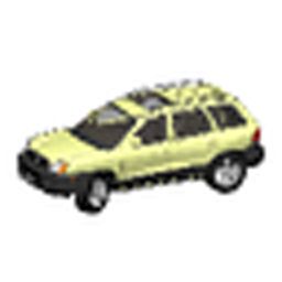
Published as a conference paper at ICLR 2023
relevant attributes), and treat pseudo-anomalies as normal as the familiar samples, as they differ only
in nuisance attributes.
Metrics. We wish not only to measure our overall anomaly detection performance but also to evaluate
the false alarm rate due to pseudo-anomalies. We therefore report our results in terms of three different
scores. Each uses two subsets of the test set and measures how well our anomaly detection algorithm
discriminates between them in terms of ROC-AUC: (i) Standard anomaly detection (AD)-Score,
which measures how accurately anomalies are detected with respect to the normal test data (both
familiar samples and pseudo-anomalies). (ii) Pseudo anomalies (PA)-Score: measures how much
pseudo-anomalies are scored as anomalous compared to familiar samples (iii) Relative abnormality
(RA)-score: measures how accurately true anomalies are detected compared to pseudo-anomalies.
5.2 R ESULTS
Compared Methods. We compared to the following methods: DN2 (Reiss et al., 2021), MeanShifted
(Reiss & Hoshen, 2021), CSI (Tack et al., 2020), SimCLR (Chen et al., 2020). A full description of
the compared methods can be found in App.(C).
Datasets. We report the results on three multi-attribute datasets based on Cars3D, SmallNORB
and Edges2Shoes. We chose these specific datasets as they are the common datasets in the field of
domain-supervised disentanglement (Gabbay & Hoshen, 2019; Kahana & Hoshen, 2022). We also
find these datasets to be non-trivial for state-of-the-art anomaly detection algorithms. Full details on
each dataset can be found in App.E.
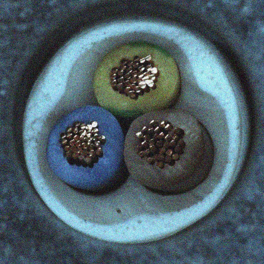
Cars3D (Reed et al., 2015). A synthetic dataset, where each image is formed using two attributes:
car model and pose. Car models are varied across different colors, shapes and, functionalities. Each
car model is observed from multiple camera angles (pose). To simulate pseudo anomalies, we
randomized for each pose a single car model and labeled it as a pseudo-anomaly. An illustration of
the dataset can be seen in Fig. 1. We can see in Tab.1 that the disentanglement approach significantly
outperforms methods that do not use any guidance to remove the nuisance attribute. We detect true
anomalies, without assigning high anomaly scores to the pseudo-anomalies significantly better than
all other methods compared. The RA-Score shows that we distinguish well between true anomalies
and pseudo-anomalies.
SmallNorb (LeCun et al., 2004). In this dataset as well we define our nuisance attribute to the
camera angles, and pseudo-anomalies are car models seen from a never-seen-before angle during test
time. We can see in Tab.2 that our approach outperforms on this dataset too. All methods utilizing
pre-trained features detect true anomalies fairly well. This is expected, as the network learns a good
representation of objects during pre-training. Our disentanglement approach significantly reduces the
tendency to score pseudo-anomalies as anomalies. CSI treats pseudo-anomalies similarly to normal
samples, but this is most likely because its representation for this dataset is not informative, and
Type-1 Type-2 Type-3 Type-4 Type-5 (Anom.)
Pose 1
Pose 4
Pose 9
Pose 17
Figure 1: Samples from the Cars3D datasets. Pseudo-anomalies are marked in green while true
anomalies are marked in red. Both pseudo-anomalies and true anomalies appear only in the test set.
7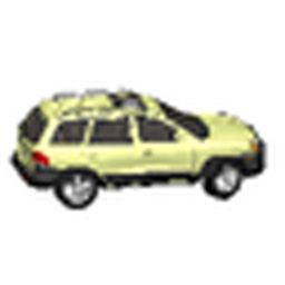
Published as a conference paper at ICLR 2023

              Table 1: Empirical Evaluation on the Cars3D Dataset (ROC-AUC)
      Dataset            Method              AD-Score (⇑) PA-Score (⇓) RA-Score (⇑)
                           SimCLR                     0.780            0.519            0.741
                             CSI                      0.606            0.579            0.538
                             DN2                      0.946            0.564            0.916
      Cars3D
                          MeanShifted                 0.943            0.595            0.917
                              Ours                    0.985            0.506            0.980

does not distinguish well between unseen data (true anomalies or pseudo-anomalies) and the familiar
samples.

                Table 2: Empirical Evaluation on the SmallNorb Dataset (ROC-AUC)
      Dataset               Method              AD-Score (⇑) PA-Score (⇓) RA-Score (⇑)
                           SimCLR                     0.805            0.728            0.638
                             CSI                      0.618            0.556            0.575
                             DN2                      0.908            0.819            0.768
    SmallNorb
                          MeanShifted                 0.948            0.870            0.811
                              Ours                    0.953            0.581            0.943

Edges2Shoes (Isola et al., 2017). This dataset contains photos of shoes and edge maps images of
the same photos. An illustration of the dataset can be seen in Fig. 2. This dataset is challenging
as the photo and sketch domains are quite far, making the nuisance attribute dominant. E.g., by
observing only sketches of boots, real photos of boots could be easily considered as anomalies without
further guidance. Our approach outperforms methods that do not remove nuisance attributes from
the representation. We observe (by the PA-score) that although the pseudo-anomalies are indeed
scored higher than normal images by our approach, their scores are still lower than the true anomalies
(demonstrated by the RA-score). Our approach significantly outperforms the baselines, showcasing
the importance of specifying and removing nuisance attributes.

            Table 3: Empirical Evaluation on the Edges2Shoes Dataset (ROC-AUC)
      Dataset             Method              AD-Score (⇑) PA-Score (⇓) RA-Score (⇑)
                           SimCLR                     0.567            0.642            0.510
                             CSI                      0.574            0.873            0.412
                             DN2                      0.500            0.631            0.455
    Edges2Shoes
                          MeanShifted                 0.486            0.790            0.386
                              Ours                    0.781            0.711            0.719

In summary, while some methods outperformed our method in terms of PA score on some experiments,
this was done by scoring both pseudo-anomalies and true anomalies as normal samples (resulting in
significantly worse AD-Score). The PA score alone can simply be optimized by a random anomaly
detector - getting ROC-AUC of 0.5. The RA-score measures the ability to distinguish true anomalies
from pseudo anomalies directly. We significantly outperform all baselines on this score.

6    D ISCUSSION & L IMITATIONS
Multi-attribute dataset. Many datasets (e.g. SmallNorb) have more than two attributes. In some
cases, we may wish to remove multiple nuisance attributes. Methods such as (Gabbay & Hoshen,
2019) very naturally extend to the case of disentangling many factors of the same dataset. These
methods operate using carefully-designed bottlenecks. Multiple attributes can be excluded by
concatenating their representation to the latent code (Gabbay et al., 2021). Our approach can be
extended to the case of multiple attributes using such methods.

                                                  8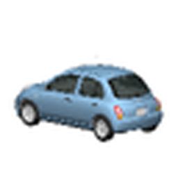
Published as a conference paper at ICLR 2023

Applying our approach to other data modalities. While this work is focused on image datasets,
disentanglement approaches may assist anomaly detection efforts in other modalities as well. This
includes modalities such as audio signals (Abeßer & Müller, 2021) or text (Cheng et al., 2020), and
also scientific data such as Single-Cell data (Hetzel et al.).

 Table 4: Empirical Evaluation on the MVTec-AD Dataset With Nuisance Attributes (ROC-AUC)
     PatchCore       No Nuis. JPEG JPEG+ Contr. Contr.+ Gauss. Gauss.+
     AD-Score (⇑)        0.991       0.848     0.860      0.914      0.915       0.895      0.900
     PA-Score (⇓)          -         0.977     0.976      0.980      0.980       0.972      0.969
     RA-Score (⇑)          -         0.701     0.725      0.833      0.836       0.796      0.806

Domain supervised disentanglement in the wild. Currently, state-of-the-art domain-supervised
disentanglement methods achieve impressive results on synthetic or curated datasets. Such methods
do not perform as well for in-the-wild datasets. As our approach heavily relies on disentanglement, it
is prone to similar limitations. As the field of disentanglement advances, the advancements can be
translated to improved anomaly detection capabilities using our approach. To evaluate the progress
of future anomaly detection methods, we also include a harder benchmark (Tab.6). We adapt a
standard anomaly detection benchmark (MVTec-AD, (Bergmann et al., 2019)), and evaluate a state-
of-the-art method (PatchCore (Roth et al., 2021)) that achieves very high accuracy on the original
data (“No Nuis.”). However, in the presence of nuisance factors, that create pseudo-anomalies in
the test set (JPEG compression, Contrast Augmentation, Gaussian noise), the anomaly detection
results significantly deteriorate. The method we proposed cannot apply to this dataset for multiple
reasons: (i) it is designed for coarse-grained rather than fine-grained AD (ii) it struggles with complex
real-world images. Extending the state-of-the-art to such datasets is an open challenge. Additional
details about this benchmark can be found in App.A.
is not solved by the methods explored in this paper (including ours), and is left for future research.
Highly biased datasets. Similarly to other disentanglement approaches, we require the distributions
of relevant attributes across nuisance domains to be somewhat similar. We have shown that our
method can work when the supports across domains are not overlapping. Still, we expect that when
the supports are highly non-overlapping the results will significantly deteriorate. Developing methods
able to disentangle domains with highly non-overlapping support is an exciting future direction.
Imperfect invariance. While our method aims to achieve invariance, the results are still imperfect.
We report the invariance and informativeness of our learned representations in Tab.11. Although far
from optimal, the method already provides significant gains for the anomaly detection task (Sec.5).
Missing and mislabeled nuisance factors. As our approach relies on labeled nuisance factors, it
might be sensitive to mislabeled nuisance labels. Although wrong labels can hinder the efforts of
most machine learning algorithms, our approach might be sensitive to two other types of errors: (i)
our technical methods rely on categorical labels for the nuisance attribute. In our experiments we
successfully address this by quantization of the continuous variable. Yet, this procedure should be
carefully examined for each application. (ii) if a user fails to identify the correct nuisance factor, our
method could not be used to remove it.
Further Discussion. Further discussion regarding Supervised vs. self-supervised pre-training
Supervised vs. self-supervised pret-raining Removing nuisance attributes with generative models

7    C ONCLUSION
We proposed a new anomaly detection setting where information is provided on a set of attributes
that are known to be irrelevant for distinguishing between normal samples and anomalies. Using
a disentanglement-based approach, we showed how this additional supervision can be leveraged
for better anomaly detection in biased datasets. As identifying irrelevant attributes is easier than
predicting in which attributes anomalies will appear, we expect further research on this new setting to
be fruitful and promising.

                                                    9
Published as a conference paper at ICLR 2023

8   ACKNOWLEDGEMENT

This research was partially supported by the Israeli Science Foundation, the Hebrew University Data
Science grants (CIDR), and the Israeli Council for Higher Education.

R EFERENCES
Jakob Abeßer and Meinard Müller. Towards audio domain adaptation for acoustic scene classification
  using disentanglement learning. arXiv preprint arXiv:2110.13586, 2021.

Paul Bergmann, Michael Fauser, David Sattlegger, and Carsten Steger. Mvtec ad–a comprehensive
  real-world dataset for unsupervised anomaly detection. In Proceedings of the IEEE/CVF conference
  on computer vision and pattern recognition, pp. 9592–9600, 2019.

Diane Bouchacourt, Ryota Tomioka, and Sebastian Nowozin. Multi-level variational autoencoder:
  Learning disentangled representations from grouped observations. In Proceedings of the AAAI
  Conference on Artificial Intelligence, volume 32, 2018.

Markus M Breunig, Hans-Peter Kriegel, Raymond T Ng, and Jörg Sander. Lof: identifying density-
 based local outliers. In Proceedings of the 2000 ACM SIGMOD international conference on
 Management of data, pp. 93–104, 2000.

Ting Chen, Simon Kornblith, Mohammad Norouzi, and Geoffrey Hinton. A simple framework for
  contrastive learning of visual representations. In International conference on machine learning, pp.
  1597–1607. PMLR, 2020.

Ting Chen, Calvin Luo, and Lala Li. Intriguing properties of contrastive losses. Advances in Neural
  Information Processing Systems, 34, 2021.

Yunqiang Chen, Xiang Sean Zhou, and Thomas S Huang. One-class svm for learning in image re-
  trieval. In Proceedings 2001 international conference on image processing (Cat. No. 01CH37205),
  volume 1, pp. 34–37. IEEE, 2001.

Pengyu Cheng, Martin Renqiang Min, Dinghan Shen, Christopher Malon, Yizhe Zhang, Yitong
  Li, and Lawrence Carin. Improving disentangled text representation learning with information-
  theoretic guidance. arXiv preprint arXiv:2006.00693, 2020.

Niv Cohen and Yedid Hoshen. Sub-image anomaly detection with deep pyramid correspondences.
  arXiv preprint arXiv:2005.02357, 2020.

Davide Cozzolino, Justus Thies, Andreas Rössler, Christian Riess, Matthias Nießner, and Luisa
  Verdoliva. Forensictransfer: Weakly-supervised domain adaptation for forgery detection. arXiv
  preprint arXiv:1812.02510, 2018.

Elliot Creager, David Madras, Jörn-Henrik Jacobsen, Marissa Weis, Kevin Swersky, Toniann Pitassi,
  and Richard Zemel. Flexibly fair representation learning by disentanglement. In International
  conference on machine learning, pp. 1436–1445. PMLR, 2019.

Ian Davidson and Selvan Suntiha Ravi. A framework for determining the fairness of outlier detection.
  In ECAI 2020, pp. 2465–2472. IOS Press, 2020.

Lucas Deecke, Lukas Ruff, Robert A Vandermeulen, and Hakan Bilen. Transfer-based semantic
  anomaly detection. In International Conference on Machine Learning, pp. 2546–2558. PMLR,
  2021.

Jia Deng, Wei Dong, Richard Socher, Li-Jia Li, Kai Li, and Li Fei-Fei. Imagenet: A large-scale
   hierarchical image database. In 2009 IEEE conference on computer vision and pattern recognition,
   pp. 248–255. Ieee, 2009.

Aviv Gabbay and Yedid Hoshen. Demystifying inter-class disentanglement. arXiv preprint
  arXiv:1906.11796, 2019.

                                                 10
Published as a conference paper at ICLR 2023
Aviv Gabbay and Yedid Hoshen. Scaling-up disentanglement for image translation. In Proceedings
of the IEEE/CVF International Conference on Computer Vision, pp. 6783–6792, 2021.
Aviv Gabbay, Niv Cohen, and Yedid Hoshen. An image is worth more than a thousand words:
Towards disentanglement in the wild. Advances in Neural Information Processing Systems, 34:
9216–9228, 2021.
Urvi Gianchandani, Praveen Tirupattur, and Mubarak Shah. Weakly-supervised spatiotemporal
anomaly detection. University of Central Florida Center for Research in Computer Vision REU,
2019.
Sachin Goyal, Aditi Raghunathan, Moksh Jain, Harsha Vardhan Simhadri, and Prateek Jain. Drocc:
Deep robust one-class classification. In International Conference on Machine Learning, pp.
3711–3721. PMLR, 2020.
Xiaoyi Gu, Leman Akoglu, and Alessandro Rinaldo. Statistical analysis of nearest neighbor methods
for anomaly detection. Advances in Neural Information Processing Systems, 32, 2019.
Dan Hendrycks and Thomas Dietterich. Benchmarking neural network robustness to common corrup-
tions and perturbations. Proceedings of the International Conference on Learning Representations,
2019.
Dan Hendrycks and Kevin Gimpel. A baseline for detecting misclassified and out-of-distribution
examples in neural networks. arXiv preprint arXiv:1610.02136, 2016.
Dan Hendrycks, Mantas Mazeika, Saurav Kadavath, and Dawn Song. Using self-supervised learning
can improve model robustness and uncertainty. Advances in Neural Information Processing
Systems, 32, 2019.
Dan Hendrycks, Xiaoyuan Liu, Eric Wallace, Adam Dziedzic, Rishabh Krishnan, and Dawn Song.
Pretrained transformers improve out-of-distribution robustness. arXiv preprint arXiv:2004.06100,
2020.
Leon Hetzel, Simon Boehm, Niki Kilbertus, Stephan Günnemann, Mohammad Lotfollahi, and
Fabian J Theis. Predicting cellular responses to novel drug perturbations at a single-cell resolution.
In Advances in Neural Information Processing Systems.
Wei-Ning Hsu, Yu Zhang, and James Glass. Unsupervised learning of disentangled and interpretable
representations from sequential data. Advances in neural information processing systems, 30,
2017.
Minyoung Huh, Pulkit Agrawal, and Alexei A Efros. What makes imagenet good for transfer
learning? arXiv preprint arXiv:1608.08614, 2016.
Phillip Isola, Jun-Yan Zhu, Tinghui Zhou, and Alexei A Efros. Image-to-image translation with
conditional adversarial networks. In Proceedings of the IEEE conference on computer vision and
pattern recognition, pp. 1125–1134, 2017.
Ananya Harsh Jha, Saket Anand, Maneesh Singh, and VSR Veeravasarapu. Disentangling factors
of variation with cycle-consistent variational auto-encoders. In Proceedings of the European
Conference on Computer Vision (ECCV), pp. 805–820, 2018.
Jeff Johnson, Matthijs Douze, and Hervé Jégou. Billion-scale similarity search with GPUs. IEEE
Transactions on Big Data, 7(3):535–547, 2019.
Jonathan Kahana and Yedid Hoshen. A contrastive objective for learning disentangled representations.
arXiv preprint arXiv:2203.11284, 2022.
Tero Karras, Samuli Laine, and Timo Aila. A style-based generator architecture for generative
adversarial networks. In Proceedings of the IEEE/CVF conference on computer vision and pattern
recognition, pp. 4401–4410, 2019.
11Published as a conference paper at ICLR 2023
James Kirkpatrick, Razvan Pascanu, Neil Rabinowitz, Joel Veness, Guillaume Desjardins, Andrei A
Rusu, Kieran Milan, John Quan, Tiago Ramalho, Agnieszka Grabska-Barwinska, et al. Overcoming
catastrophic forgetting in neural networks. Proceedings of the national academy of sciences, 114
(13):3521–3526, 2017.
Yann LeCun, Fu Jie Huang, and Léon Bottou. Learning methods for generic object recognition with
invariance to pose and lighting. Proceedings of the 2004 IEEE Computer Society Conference on
Computer Vision and Pattern Recognition, 2:II–104 Vol.2, 2004.
Wei-Yu Lee and Yu-Chiang Frank Wang. Learning disentangled feature representations for anomaly
detection. In 2020 IEEE International Conference on Image Processing (ICIP), pp. 2156–2160.
IEEE, 2020.
Lishuai Li, R John Hansman, Rafael Palacios, and Roy Welsch. Anomaly detection via a gaussian
mixture model for flight operation and safety monitoring. Transportation Research Part C:
Emerging Technologies, 64:45–57, 2016.
Xingchao Peng, Zijun Huang, Ximeng Sun, and Kate Saenko. Domain agnostic learning with
disentangled representations. In International Conference on Machine Learning, pp. 5102–5112.
PMLR, 2019.
Pramuditha Perera and Vishal M Patel. Learning deep features for one-class classification. IEEE
Transactions on Image Processing, 28(11):5450–5463, 2019.
Tomáš Pevnỳ. Loda: Lightweight on-line detector of anomalies. Machine Learning, 102(2):275–304,
2016.
Alec Radford, Jong Wook Kim, Chris Hallacy, Aditya Ramesh, Gabriel Goh, Sandhini Agarwal,
Girish Sastry, Amanda Askell, Pamela Mishkin, Jack Clark, et al. Learning transferable visual
models from natural language supervision. In International Conference on Machine Learning, pp.
8748–8763. PMLR, 2021.
Scott E Reed, Yi Zhang, Yuting Zhang, and Honglak Lee. Deep visual analogy-making. Advances in
neural information processing systems, 28, 2015.
Tal Reiss and Yedid Hoshen. Mean-shifted contrastive loss for anomaly detection. arXiv preprint
arXiv:2106.03844, 2021.
Tal Reiss, Niv Cohen, Liron Bergman, and Yedid Hoshen. Panda: Adapting pretrained features for
anomaly detection and segmentation. In Proceedings of the IEEE/CVF Conference on Computer
Vision and Pattern Recognition, pp. 2806–2814, 2021.
Karsten Roth, Latha Pemula, Joaquin Zepeda, Bernhard Schölkopf, Thomas Brox, and Peter Gehler.
Towards total recall in industrial anomaly detection. arXiv preprint arXiv:2106.08265, 2021.
Lukas Ruff, Robert Vandermeulen, Nico Goernitz, Lucas Deecke, Shoaib Ahmed Siddiqui, Alexander
Binder, Emmanuel Müller, and Marius Kloft. Deep one-class classification. In International
conference on machine learning, pp. 4393–4402. PMLR, 2018.
Lukas Ruff, Jacob R Kauffmann, Robert A Vandermeulen, Grégoire Montavon, Wojciech Samek,
Marius Kloft, Thomas G Dietterich, and Klaus-Robert Müller. A unifying review of deep and
shallow anomaly detection. Proceedings of the IEEE, 109(5):756–795, 2021.
Mohammadreza Salehi, Hossein Mirzaei, Dan Hendrycks, Yixuan Li, Mohammad Hossein Rohban,
and Mohammad Sabokrou. A unified survey on anomaly, novelty, open-set, and out-of-distribution
detection: Solutions and future challenges. arXiv preprint arXiv:2110.14051, 2021.
Shubhranshu Shekhar, Neil Shah, and Leman Akoglu. Fairod: Fairness-aware outlier detection. In
Proceedings of the 2021 AAAI/ACM Conference on AI, Ethics, and Society, pp. 210–220, 2021.
Jihoon Tack, Sangwoo Mo, Jongheon Jeong, and Jinwoo Shin. Csi: Novelty detection via contrastive
learning on distributionally shifted instances. In Advances in Neural Information Processing
Systems, 2020.
12Published as a conference paper at ICLR 2023
David MJ Tax and Robert PW Duin. Support vector data description. Machine learning, 54(1):45–66,
2004.
Sjoerd Van Steenkiste, Francesco Locatello, Jürgen Schmidhuber, and Olivier Bachem. Are disen-
tangled representations helpful for abstract visual reasoning? Advances in Neural Information
Processing Systems, 32, 2019.
Tongzhou Wang and Phillip Isola. Understanding contrastive representation learning through align-
ment and uniformity on the hypersphere. In International Conference on Machine Learning, pp.
9929–9939. PMLR, 2020.
Zongze Wu, Dani Lischinski, and Eli Shechtman. Stylespace analysis: Disentangled controls for
stylegan image generation. In Proceedings of the IEEE/CVF Conference on Computer Vision and
Pattern Recognition, pp. 12863–12872, 2021.
Jingkang Yang, Kaiyang Zhou, Yixuan Li, and Ziwei Liu. Generalized out-of-distribution detection:
A survey. arXiv preprint arXiv:2110.11334, 2021.
Aron Yu and Kristen Grauman. Fine-grained visual comparisons with local learning. In Proceedings
of the IEEE Conference on Computer Vision and Pattern Recognition (CVPR), June 2014.
Hongjing Zhang and Ian Davidson. Towards fair deep anomaly detection. In Proceedings of the 2021
ACM Conference on Fairness, Accountability, and Transparency, pp. 138–148, 2021.
Jun-Yan Zhu, Zhoutong Zhang, Chengkai Zhang, Jiajun Wu, Antonio Torralba, Josh Tenenbaum,
and Bill Freeman. Visual object networks: Image generation with disentangled 3d representations.
Advances in neural information processing systems, 31, 2018.
Roland S Zimmermann, Yash Sharma, Steffen Schneider, Matthias Bethge, and Wieland Brendel.
Contrastive learning inverts the data generating process. In International Conference on Machine
Learning, pp. 12979–12990. PMLR, 2021.
13Published as a conference paper at ICLR 2023
A MVT EC -AD BASED A NOMALY D ETECTION W ITH N UISANCE FACTORS
We wish to evaluate the NAGAD setting on a more realistic benchmark. Therefore, we adapt the
MVTec-AD benchmark to include nuisance factors. We extend the test set of each class to include
pseudo-anomalies: normal test samples that underwent an augmentation simulating a different image
source (see Sec.A.1). We also include the true anomalies twice: once in their original form, and once
with the augmentation. We down-sample the true anomalies by a factor of 5 to keep the class sizes
relatively balanced. As can be seen in Tab.A including pseudo-anomalies significantly deteriorates
the anomaly detection capabilities with respect to the original data. The pseudo-anomalies differ from
the normal data (Tab.A, PA-score) and are often considered more anomalous than the true anomalies
(Tab.A, RA-Score).
To allow future methods the ability to adapt, and be more invariant to the nuisance variation, we also
include a version with an extended dataset in our benchmark (Tab.A, JPEG+; Contr.+; Gauss.+). In
this version the normal training data include both the original and augmented normal data, from two
unrelated MVTec classes (“transistor” & “zipper”). Using the labels on the nuisance variation for
these classes, we expect future methods to be able to pay less attention to the nuisance attribute. We
therefore do not include the MVTec-AD classes “transistor” & “zipper” in our average image-level
ROC-AUC. As the other discussed methods perform less well also on the original MVTec-AD dataset,
we do not include their results.
A.1 AUGMENTATIONS AS N UISANCE ATTRIBUTES
To simulate the nuisance attribute, we consider three augmentations, chosen from the augmentations
used by Hendrycks & Dietterich (2019). For each chosen augmentation we specify its severity degree
as defined there. We consider the following augmentations:
JPEG - JPEG compression artifacts taken by severity degree 5, compressing each image to 7% of its
original size.
Contrast - Decrease of contrast for each image (severity degree 3).
Gaussian Noise - Blurring each image (severity degree 5). Specifically, the blurring gaussian kernel
has a standard deviation of 3.
We illustrate the chosen augmentations on one image in Fig.A.1.
B F URTHER D ISCUSSION
Supervised vs. self-supervised pre-training. Many top-performing approaches (including ours)
rely on externally-pretrained weights for initializing their neural networks. Pre-trained weights
implicitly provide useful guidance regarding the relevant attributes we should focus on, and the
ones we may wish to ignore (e.g. low-level image information). Different pre-trained networks
provide different relevant/nuisance attribute splits. We found that pre-trained weights obtained from
supervised classification on external datasets such as ImageNet, tend to emphasize the main object
featured in the center of the image, and are more invariant to other attributes. Representations
Original Gaussian Noise Contrastive JPEG
A glossary of the augmentations used to create the nuisance factors in Tab.6: An original image,
Gaussian noise augmentation, Contrastive augmentation, and JPEG Compression augmentation.
14Published as a conference paper at ICLR 2023
learned by self-supervised pre-training on external datasets are affected both by the dataset and by the
augmentation used for its contrastive learning. Therefore they may have different inductive biases.
Augmentations. Different methods may require augmented images to be similar or dissimilar to the
original image (Chen et al., 2020; Tack et al., 2020). This choice tends to have a strong effect on the
results. E.g., a network trained to be rotation invariant may fail when the relevant attributes include
the image orientation angle. Our approach only uses simple augmentations such as Gaussian blurring,
saturation, and crops. We expect these augmentations not to restrict the anomalies detectable in the
vast majority of cases. In general, augmentations should be carefully inspected when deploying
anomaly detection methods in practice.
Removing nuisance attributes with generative models. Recently, generative models e.g. StyleGAN
(Karras et al., 2019) have been able to learn very powerful representations for several data types,
particularly images of faces. Their representations exhibit a certain level of disentanglement (Wu
et al., 2021). When available, such models can be utilized for removing nuisance attributes in a
similar approach to ours.
C C OMPARED M ETHODS
DN2 (Reiss et al., 2021). A simple but effective approach fully reliant on pre-training. It uses an
ImageNet-pretrained network to extract representations for each image. Each test image is scored
using kNN density estimation similarly to our approach. MeanShifted (Reiss & Hoshen, 2021).
A recent method that achieves state-of-the-art performance on standard anomaly benchmarks. It
uses a modified contrastive learning loss to adapt its feature to the normal train set. This method
uses the same pre-trained network as our method to initialize the features. It then uses a kNN for
anomaly scoring. CSI (Tack et al., 2020). A strong self-supervised anomaly detection method that
does not rely on pre-training. It uses two types of augmentations: fine augmentations simulating
positive contrastive loss samples, and domain shifts simulating negative samples. Anomaly scoring
is performed using an ensemble of similarity scores based on the learnt features. SimCLR (Chen
et al., 2020). An ablation of our approach that trains a single contrastive loss rather than a different
contrastive loss for each domain. We score the anomalies similarly to our approach.
D I MPLEMENTATION D ETAILS
D.1 D ISENTANGLEMENT MODULE
We use most of the parameters as in the DCoDR paper (Kahana & Hoshen, 2022) for our disentangle-
ment module. All images were used in a 64 × 64 resolution. For the contrastive temperature, we use
τ = 0.1 for all the datasets. We scale down the loss Lrec by a factor of 0.3.
Boots Sandals Shoes Slippers (Anom.)
Photos
Sketches
Figure 2: Samples from the Edges2Shoes datasets. Pseudo-anomalies are marked in green while true
anomalies are marked in red. Both pseudo-anomalies and true anomalies appear only in the test set.
15Published as a conference paper at ICLR 2023
Architecture. We used a ResNet50 encoder pre-trained on image classifications. In accordance with
previous works, we add 3 fully-connected layers to the encoder for the SmallNorb dataset (Gabbay &
Hoshen, 2019; Kahana & Hoshen, 2022). For the perceptual loss of the generator we used a VGG
network pre-trained on ImageNet.
Optimization. We use 200 training epochs. In each batch we used 32 images from 4 different
nuisance classes (a batch size of 128, in total). We used a learning rates of 1 · 10−4 and 3 · 10−4 for
the encoder and generator (respectively).
Augmentation. We used Gaussian blurring (kernel_size = 5, σ = 1), high contrast (contrast
= (1.8, 3.0)), and high saturation (saturation = (1.8, 3.0)) for our augmentation. For Edges2Shoes
we used only Gaussian Blurring. For the SimCLR (Chen et al., 2020) contrastive learning (both in
our approach and the baseline), we follow DCoDR by only augmenting the original image once, and
comparing the augmented and the original views encodings. This is in contrast to SimCLR which
compares two augmented views instead.
Baselines. We ran all the baselines using the same ResNet50 backbone network we used. As
CSI (Tack et al., 2020) performance deteriorated when using ResNet50, we ran it with the original
ResNet18 backbone used by the authors.
D.2 H YPERPARAMETER TUNING
As we aim to detect anomalies without relying on any labelled anomalous samples, we used all
the baselines with their default parameters. As DCoDR (Kahana & Hoshen, 2022) uses a different
temperature parameter for each dataset, we used τ = 0.1 for all datasets.
D.3 S CORING MODULE
We use faiss (Johnson et al., 2019) kNN implementation, using k = 1.
E DATASETS
We label each sample as either normal, true anomaly, or pseudo-anomaly as detailed below. We
include only true anomalies and pseudo-anomalies in the test set, and split the normal samples
between the training set and the test set (85%/15% train/test split). To simulate anomalies in the
dataset, we first designate true anomalies as described in Sec.5. We then chose combinations of
normal classes and the nuisance attribute to designate pseudo anomalies. We used the following
random combinations for pseudo anomalies:
Cars3D: We define true anomalies as images of 5 (randomly selected) car models. The nuisance
attributes are defined in Tab.5.
Table 5: Cars3D Pseudo Anomalies Selection
Azimuth Object Type Azimuth Object Type
0 173 12 48
1 16 13 66
2 75 14 32
3 23 15 153
4 44 16 128
5 78 17 120
6 108 18 38
7 7 19 172
8 167 20 106
9 182 21 4
10 99 22 175
11 78 23 111
16You can also read