A Tweet Sentiment Classification Approach Using a Hybrid Stacked Ensemble Technique
←
→
Page content transcription
If your browser does not render page correctly, please read the page content below
information

Article
A Tweet Sentiment Classification Approach Using a Hybrid
Stacked Ensemble Technique
Babacar Gaye, Dezheng Zhang and Aziguli Wulamu *

                                          School of Computer and Communication Engineering, University of Science and Technology Beijing,
                                          Beijing 100083, China; babacargaye92@gmail.com (B.G.); zdzchina@126.com (D.Z.)
                                          * Correspondence: aziguli@ustb.edu.cn

                                          Abstract: With the extensive availability of social media platforms, Twitter has become a significant
                                          tool for the acquisition of peoples’ views, opinions, attitudes, and emotions towards certain entities.
                                          Within this frame of reference, sentiment analysis of tweets has become one of the most fascinating
                                          research areas in the field of natural language processing. A variety of techniques have been devised
                                          for sentiment analysis, but there is still room for improvement where the accuracy and efficacy
                                          of the system are concerned. This study proposes a novel approach that exploits the advantages
                                          of the lexical dictionary, machine learning, and deep learning classifiers. We classified the tweets
                                          based on the sentiments extracted by TextBlob using a stacked ensemble of three long short-term
                                          memory (LSTM) as base classifiers and logistic regression (LR) as a meta classifier. The proposed
                                          model proved to be effective and time-saving since it does not require feature extraction, as LSTM
                                          extracts features without any human intervention. We also compared our proposed approach with
                                          conventional machine learning models such as logistic regression, AdaBoost, and random forest.
                                We also included state-of-the-art deep learning models in comparison with the proposed model.

                                          Experiments were conducted on the sentiment140 dataset and were evaluated in terms of accuracy,
Citation: Gaye, B.; Zhang, D.;            precision, recall, and F1 Score. Empirical results showed that our proposed approach manifested
Wulamu, A. A Tweet Sentiment              state-of-the-art results by achieving an accuracy score of 99%.
Classification Approach Using a
Hybrid Stacked Ensemble Technique.
                                          Keywords: machine learning; classification; ensemble learning; sentiment analysis
Information 2021, 12, 374.
https://doi.org/10.3390/
info12090374

                                          1. Introduction
Academic Editor: Rodrigo Agerri
                                                Advances in internet technology and the continuous development of web 2.0 is
Received: 20 August 2021                  resulting in the production of a substantial amount of data daily. The availability of a
Accepted: 8 September 2021                plethora and variety of social media platforms increased the connectivity among social
Published: 14 September 2021              media users which changes the prevalent viewpoint of socialization, personalization, and
                                          networking. For the fourth quarter of 2020, an estimated number of 1.8 billion users were
Publisher’s Note: MDPI stays neutral      active on Facebook each day [1]. This is in addition to Facebook ancillary services like
with regard to jurisdictional claims in   Instagram, WhatsApp, and messenger each of which have active users amounting to 1
published maps and institutional affil-   billion on a monthly basis [2]. Similarly, according to third-party analysis, other social
iations.                                  media platforms such as iMessage owned by Apple, WeChat by Tencent, and YouTube by
                                          Google, which is no longer exclusive, are now members of the 1 billion-per-month-active-
                                          user-club. Furthermore, 75% of internet users now regularly use at least one social media
                                          platform [3]. From a purely technical standpoint, increased accessibility has provided new
Copyright: © 2021 by the authors.         opportunities and challenges by encouraging users to share their views, emotions, and
Licensee MDPI, Basel, Switzerland.        opinions, in addition to consuming services [4,5]. One of the fast-growing and impactful
This article is an open access article    social media networks is Twitter, on which users can read, post, and update short text
distributed under the terms and           messages termed as ‘tweets’ which enable Twitter users to communicate their views,
conditions of the Creative Commons        opinions, and sentiments about a particular entity. These sentiment-bearing tweets play
Attribution (CC BY) license (https://     a vital role in many areas, for instance, social media marketing [6], academics [7], and
creativecommons.org/licenses/by/          election campaign news [6].
4.0/).

Information 2021, 12, 374. https://doi.org/10.3390/info12090374                                       https://www.mdpi.com/journal/information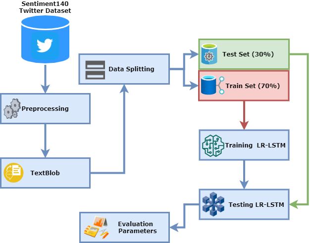
Information 2021, 12, 374                                                                                            2 of 19

                                  Sentiment analysis aims at categorizing and determining the polarity of a subjective
                            text at phrase, sentence, or document level [8]. It has a variety of applications in vari-
                            ous fields, including e-commerce, politics, entertainment, and health care to name a few.
                            For instance, sentiment analysis can help companies to track customer perceptions about
                            their products, it can also assist customers in selecting the best product based on public
                            opinion [9]. While sentiment analysis has various applications and implementations in a
                            variety of fields, it comes with diverse issues and challenges related to Natural Language
                            Processing (NLP). Recent research related to sentiment analysis is still afflicted by technical
                            and theoretical complexity which limit its inclusive accuracy in sentiment detection [10].
                            Hussein et al. [11] investigated the challenges of sentiment analysis and their effects on the
                            accuracy of the results. The experimental results substantiated that accuracy is a consider-
                            able challenge in the conduction of sentiment analysis. It also demonstrates that accuracy is
                            affected by several challenges, such as handling sarcasm, negation, abbreviations, domain
                            dependence, bi-polar words, etc.
                                  As for sentiment analysis of tweets, the key task is to classify the divergence between
                            opinion-bearing tweets as either negative or positive. Sentiment analysis of tweets comes
                            with its challenges. People tend to use informal language in their tweets, which might
                            heighten the risk of not detecting the overall sentiment of the text [12]. Some tweets
                            are short text, which may carry little contextual information which provides inadequate
                            indications of sentiment [13]. Understanding the sentiments of tweets containing acronyms
                            and abbreviations is also an immense challenge for the computer. Attributable to these
                            challenges, a growing interest of researchers is classifying the sentiments of tweets.
                                  Sentiments of tweets can be investigated using three approaches: (I) a machine learn-
                            ing (ML) approach which utilizes learning models for classification of sentiments; (II) a
                            rule-based approach which uses either corpus-based sentiment lexicons, publicly available
                            sentiment lexicons, or lexical dictionary for extraction of sentiments; and (III) a hybrid
                            approach which combines the ML approach and rule-based approach. Consequently, deep
                            learning approaches, as integrated into a large number of researches, have shown their
                            significance in sentiment analysis [14], computer vision [15], and speech recognition [16].
                            Consequently, the authors of [17] showed that integrating ConvBiLSTM, a deep learning
                            model, produced more effective and robust results in analyzing sentiments of tweets. They
                            utilized a convolution neural network (Conv) for extraction of local features and bidirec-
                            tional long short-term memory (BiLSTM) to capture the long-distance dependencies and
                            classified tweets with 91.13% accuracy. In line with the above, another research integrated
                            deep learning models in the sentiment classification of tweets which resulted in more
                            accurate results as compared to conventional ML models [18].
                                  The Sentiment140 dataset is utilized in this study which contains 1.6 million tweets,
                            among which 800,000 tweets are negative tweets and 800,000 tweets are annotated as
                            positive. Tweets in this dataset were originally annotated by considering the emoticons, for
                            instance, tweets with happy emoticons were considered as positive and tweets containing
                            sad emoticons were considered negative [19]. This study proposes that annotating tweets
                            using a lexical dictionary generates more correlated features for more accurate sentiment
                            classification of tweets. For this purpose, the current study proposes a novel approach that
                            leverages the benefits of a lexical dictionary from the rule-based approach and learning
                            models from the ML approach for the sentiment classification of tweets.
                                  Key contributions of this study are summarized as follows:
                            •    This study explores the viability of the implementation of a lexical dictionary and
                                 evaluates the potency of a stacked ensemble for the sentiment classification of tweets.
                            •    A lexical dictionary, namely TextBlob, is integrated for sentiment annotation of tweets.
                                 TextBlob returns a float value within a range of “+1.0” and “−1.0” which represents
                                 the sentiment orientation of the text. Here, “+1.0” corresponds to positive, and “−1.0”
                                 corresponds to negative sentiments. We set the threshold value to “0” which indicates
                                 that output values greater than “0” will be regarded as positive tweets and vice versa.
Information 2021, 12, 374 3 of 19
• Three feature engineering approaches are integrated and evaluated in this study
including term frequency-inverse document frequency (TF-IDF), bag of words (BOW),
and a union of BOW and TF-IDF.
• A novel stacked ensemble of the ML model, logistic regression (LR), and a deep
learning model, LSTM, is proposed for sentiment classification of tweets. LR works
best with binary classification tasks; on the other hand, LSTM is the best choice for
remembering the long-term dependencies of larger datasets. Thus, the proposed
stacked ensemble harnesses the proficiency of combining the predictions made by
three LSTMs as base learners using LR as a meta learner.
• A diverse range of experimentation is carried out in this study to compare the per-
formance of the proposed approach with conventional state-of-the-art ML models
including random forest (RF), AdaBoost (ADB), and logistic regression (LR). More-
over, this study also compares the performance of models using original sentiments
of tweets with sentiments extracted by TextBlob.
• We also compare the performance of our proposed approach with correlated studies
carried out on the sentimnet140 dataset for the sentiment classification of tweets.
The remainder of the paper is organized as follows: Section 2 explores sentiment
analysis-related work which gives a brief description of previous studies. Section 3 briefly
describes the dataset along with preprocessing techniques utilized to create clean data. It
also explains the techniques and algorithms utilized in this research to conduct experiments.
Section 4 presents a detailed discussion and analysis of the results. Section 5 is comprised
of the conclusion and future direction.
2. Related Work
In the field of text classification, there is a wide scope for analyzing sentiments, and
many researchers have studied the mechanism of sentiment analysis by identifying emo-
tions contained in the text [20,21]. Ankit and Saleena [22] carried out Twitter sentiment
analysis by integrating an ensemble of Naïve Bayes (NB), Random Forest (RF), Support
Vector Machine (SVM), and Logistic Regression (LR) models with BOW as a feature ex-
traction technique. The authors proposed a two-fold study in which they first predicted
the sentiment score of the tweet and, in the second phase, they predicted the polarity of
the tweet based on sentiment score. They utilized four datasets including sentiment 140,
HCR (Health Care Reforms), the Frist GOP debate Twitter Sentiment dataset, and Twitter
sentiment analysis dataset for analysis of the proposed approach. The results showed that
the proposed ensemble learning classifier performs better than the stand-alone classifiers.
Onan et al. [23] proposed a multi-objective weighted voting ensemble classifier for text
sentiment classification. Their proposed system incorporates Bayesian Logistic Regression
(BLR), Linear Discriminant Analysis (LDA), NB, LR, and SVM as base learners whose
performance in terms of sensitivity and security determines the weighted adjustment.
Different classification tasks which include sentiment analysis, software defect prediction,
spam filtering, credit risk modeling, and semantic mapping suggest that their proposed
system outperforms the conventional ensemble learning models. The highest accuracy of
98.86% is achieved in the software defect detection task on a dataset containing details
of laptops.
Rustam et al. [24] proposed a voting classifier (VC) for the sentiment analysis of tweets.
VC comprises logistic regression (LR) and an SGDC (stochastic gradient descent classifier)
which produces prediction under soft voting. In their study, they classified the tweets into
three classes (positive, negative, and neutral). Different ML classifiers were also tested
on the “twitter-airline-sentiment” dataset. Their study investigated the role of feature
extraction techniques like TF, TF-IDF, and word2vec on classification accuracy. LSTM, a
deep learning model, was also used and it achieved an accuracy lower than ML models.
The accuracy achieved by the voting classifier is 78.9% and 79.1% with TF and TF-IDF
feature extraction.Information 2021, 12, 374 4 of 19
Umer et al. [25] conducted sentiment analysis of tweets using an ensemble of a
Convolutional Neural Network (CNN) and LSTM. As an ML classifier does not perform
well on the vast amount of data, to overcome this limitation, they advised use of a Deep
Learning-based ensemble system. They evaluated their proposed approach on three
different datasets. They integrate feature extraction methods such as word2vec and TF-IDF.
Results showed that the CNN-LSTM achieved higher accuracy than other classifiers. They
also compared the performance of the (CNN-LSTM) proposed model with the other deep
learning models which authenticated the proposed approach.
Stjanovski et al. [26] used the deep CNN approach to perform experiments on senti-
ment analysis on Twitter data. The proposed CNN was trained on the top most pre-trained
word embeddings derived from large text corpora using unsupervised learning, which
was further used with the dropout layer, softmax layer and two fully connected layers, and
multiple varying windowed filters. The results show that the pre-trained word vectors
are very effective on Twitter corpora for the unsupervised learning phase. They used the
Twitter 2015 dataset and achieve an F1 Score of 64.85%.
Jianqiang et al. [27] suggested a deep learning-based system to classify tweets into
negative and positive sentiments. The authors named the system global vector (Glove)
depth CNN (DCNN). For sentiment features, the authors concatenated the pre-trained
N-gram features and word embedding features as feature vectors. Moreover, they captured
contextual features by using a recurrent structure and used CNN for the representation of
text. Their proposed system achieved the highest accuracy of 85.97% on the STSGd dataset.
Santos et al. [28] recommended a deep convolutional neural network that uses char-
acter level to sentence level information to deploy sentiment classification for short texts.
They used two datasets in their study; the maximum accuracy they have achieved was
86.4% on the ST’s corpus.
Ishaq et al. [29] advocated a deep neural network-based model for hotel review
sentiments given by the guests of the hotel. The authors evaluated their proposed approach
in terms of binary class classification and multi-class classification including 3 classes and
10 classes. The results showed that a maximum accuracy of 97% is achieved by LSTM on
binary class classification.
Sentiment classification using deep learning models is highly impacted by the struc-
ture of the data under consideration. In this regard, three CNN-based and five RNN-based
deep neural networks were employed and compared in a study to exploit significant
implications for the development of a maximized sentiment classification system. The
study concluded that, the larger the training data size, the higher the accuracy of the model.
They also investigated the character-level and word-level input structure of the data on
the models which showed that a word-level structure makes the model learn the hidden
patterns more accurately as compared to the character-level structure of input data [30].
Consequently, a hybrid sentiment classification model leveraging the benefits of word
embedding techniques along with deep learning models is proposed in a study [31]. The
authors combined the FastText embedding with character embedding which are fed as an
input to the proposed hybrid of CNN and BiLSTM which achieved the highest accuracy
score of 82.14%.
Another study investigated the deep learning model CNN-LSTM for Twitter sentiment
analysis [32]. Their method first utilized unlabeled data to pre-train word embeddings
with the subset of data, along with distant supervision and fine-tuning. Their proposed
system is based on the number of ensembles of CNN and LSTM networks used in the
classification of the tweets. They used the SemEval-2017 twitter dataset for evaluation
of the proposed approach. Using an ensemble of 10 CNN and 10 LSTM networks, they
achieved an accuracy of 74.8%.
3. Materials and Methods
This study aims to classify the sentiments of tweets by proposing a two-fold method.
It first focuses on extracting the sentiments of the tweets using a lexical dictionary, andInformation 2021, 12, 374 5 of 19
then it classifies the tweets into positive and negative. The proposed approach involves the
usage of various techniques which are briefly described in the following section.
3.1. Dataset
Sentiment140 is the dataset utilized for carrying out the diverse range of experiments
in this study and was acquired from Kaggle which is a public repository for benchmark
datasets [33]. The dataset consists of 1.6 million tweets which were extracted using Twitter
search API. It is a well-balanced dataset comprising 0.8 million positive and 0.8 million
negative tweets. The tweets in this dataset are labeled as 0 which corresponds to negative
sentiment and 4 which corresponds to positive sentiment. Manually annotating the tweets
would have been a labor-intensive and time-consuming task due to the quantity. The
authors of the dataset annotated the tweets by considering the emoticons’ noise for the
prediction of the tweet as positive or negative. The dataset consists of six features which
are listed and described in Table 1. A few samples of tweets from the dataset are shown in
Table 2.
Table 1. Dataset Description.
Features Description
target Sentiment label corresponding to each tweet. (0 = negative, 4 = positive)
id Tweet ID
date Date on which the tweet was posted.
flag The query (lyx). If there is no query, then this value is NO QUERY.
user Username of the person who posted the tweet.
text Text written in the tweet.
Table 2. Tweet sample from the dataset.
No. Target Text
@Kenichan I dived many times for the ball. Managed to save 50% The rest
1 0
go out of bounds
2 0 @octolinz16 It counts, Idk why I did either. you never talk to me anymore
3 4 @ElleCTF I would like to call you at night after dinner
3.2. Data Pre-Processing
Data extracted from online platforms are largely unstructured or semi-structured such
that they contain unnecessary data which are insignificant for the analysis. This makes
pre-processing of the data a very important step in cleaning the data of redundant and
noisy material. It also impacts the performance of the ML models as stated by the authors
of [24]. An effective pre-processing method can reduce the size of the featured set extracted
from the dataset from 30% to 50%, which leaves behind only significant features which
are highly correlated with the target value. Furthermore, a large dataset necessitates more
time for training, and stop words, punctuations, numeric values, and data that are not
correlated with the analysis reduce the accuracy of the prediction. Thus, pre-processing is
essential to save computing resources and makes it easier for the ML models to train more
effectively, providing precise prediction [34].
Pre-processing of data integrates various steps such as data cleaning which involves
removing numbers, usernames, punctuations, stop words, lower case transformation, and
stemming which are described as follows:
Data Cleaning
Numbers and punctuation do not impact the sentiment of the tweet thus making
them unnecessary for sentiment classification of tweet [35]. Similarly, usernames are nouns
that are not relevant for the sentiment classification of text. Along the lines of this, stop
words which refer to the most common words in the text, only add computer overheadInformation 2021, 12, 374 6 of 19
and are not valuable for the text analysis. In this step, we removed numbers, punctuation,
usernames, and stop words from the tweets.
Lower Case Transformation
After the cleaning of unnecessary data, the text tweets are converted to lower case.
Machine learning models are case sensitive; therefore, the same words with the upper or
lower case will be considered as different words. For instance, “Boy” and “boy” will be
treated as two different words by statistical models as they will count the occurrence of
each word separately [36]; this impairs the efficiency of the classifier if case normalization
is not carried out.
Stemming
Stemming involves the conversion of words into their root forms by deleting affixes
from the words [24]. For instance, small, smaller, and smallest are variations of the root
word “small” with the same meaning. By the process of stemming, the complexity of the
textual feature is reduced, which enhances the learning ability of the classifier. Sample
tweets from the dataset before and after pre-processing are illustrated in Table 3.
Table 3. Sample tweets after preprocessing.
Sr. Sample Tweets Pre-Processed Tweets
@ehfu Want to accept credit cards ? Credit
1 want accept credit card credit approve check
approved no checks do it now 1234
@rtew Newyork will go long in investment as newyork go long investment other city go
2
other cities going long long newyork
3.3. TextBlob
TextBlob is a publicly available lexical dictionary that offers a simple API for carrying
out natural language processing (NLP) tasks [37]. It is a python library that integrates two
modules such as NaiveBayesAnalyzer (a classifier trained on a corpus of movie reviews)
and PatternAnalyzer (integrates pattern libraries). In this study, we incorporated the Pat-
ternAnalyzer for carrying out sentiment annotation tasks. TextBlob outputs float values
of the sentiment score of the text along with its subjectivity score. In this study, we only
included sentiment scores in our experiments. Sentiment scores range from +1.0 to −1.0,
where +1.0 refers to positive sentiment and −1.0 refers to negative sentiment. The authors
of [38] integrated TextBlob in carrying out sentiment classification of user reviews. The study
concluded that the feature set generated by TextBlob boosted the performance of ML models.
TextBlob extracted a total of positive tweets and the rest were regarded as negative
tweets by TextBlob. Table 4 shows the number of positive and negative tweets predicted by
TextBlob in comparison to the original sentiments. We used positive and negative tweets
for experiments, as we discard neutral tweets to make the dataset binary and make a fair
comparison of models on the original dataset. Table 5 shows the sample tweets with their
corresponding original sentiment and sentiments predicted by TextBlob.
Table 4. TextBlob sentiment ratio.
Sentiment Count
Positive 686,142
Negative 319,374
Neutral 594,484
Table 5. Sample of tweets with corresponding original sentiments and sentiments extracted by
TextBlob.
Sr. Tweets Original TextBlob
2 I need a hug Negative Positive
3 laying in bed with no voice.. Negative Positive
4 I’m tired now so... I’m going to bed...goodnight...? Positive NegativeInformation 2021, 12, 374 7 of 19
3.4. Feature Extraction Techniques
Feature extraction is a method of developing meaningful features or vectors from the
textual data for ML models to understand more effectively [39]. As stated by Heaton [40],
feature extraction can uplift the efficacy of the ML models. The current study incorporates
three feature extraction techniques including TF-IDF, BOW, Feature union (TF-IDF + BOW)
which are described as follows:
3.4.1. Bag of Words (BOW)
BOW is a feature extraction technique that models textual data by describing the
frequency of occurrence of words in a document. BOW involves two main things, including
a dictionary of familiar words and a measure of the existence of those words in the
document irrespective of their place in the text. The vocabulary size of BOW is depended
on the number of words in the document. It is a collection of words and features, where
every feature is assigned a value that represents the occurrence of that feature [41].
3.4.2. Term Frequency Inverse Document Frequency (TF-IDF)
This is a feature extraction technique that is used to extract features from data. TF-IDF
is widely used for Text analysis and music information retrieval [42]. In TF-IDF each term
in the document is given a weight based on its term frequency (TF) and inverse document
frequency (IDF) [24,43]. The term with the highest weight score is considered an important
term [44]. It computes the weight of each term by using the formula below:
N
Wi,j = TFi,j ( ) (1)
D f ,t
Here N is the total number of documents in the corpus, D f ,t is the number of doc-
uments containing the term t, and TFi,j is the number of occurrences of term t in a
document d.
3.4.3. Feature Union
Feature union concatenates the feature sets extracted by several feature extraction
techniques resulting in a larger feature set for the training of machine learning classifiers.
In this study, the union of TF-IDF and BOW feature sets is integrated into a single feature
set on the criteria of end-to-end concatenation. The resulting concatenated set provides
the advantage of autonomous fitting of data to each concatenated vectorizer, which in this
study is CountVectorizer() and TfidfVectorizer(). The feature union can be computed in
this study as:
( TFIDF + BOW ) = ( Feature set o f BOW ) U ( Feature set o f TFIDF ) (2)
3.5. Machine Learning Models
Three ML models are integrated in this study to conduct sentiment classification of
tweets including RF, ADB, and RF. ML models undergo the training and testing phase to
carry out classification tasks. Training of these models is conducted by integrating different
hyper-parameter settings for each model which were optimized under the criteria of the
hit and trial method. The optimized hyper-parameter for each model is shown in Table 6.
Table 6. Machine Learning Models Hyper-parameter Settings.
Models Hyper-Parameter Settings
RF max_depth = 300, random_state = 42, n_estimators = 300
LR C = 3.0, multi_class = ‘ovr’, solver = ‘liblinear’, random_state = 42
ADB random_state = 42, n_estimators = 300Information 2021, 12, 374 8 of 19
3.5.1. Random Forest (RF)
RF is a tree-based classifier in which every tree is the result of a random vector from
the input vector. Firstly, RF develops a forest by producing multiple decision trees on
random features. Then it aggregates voting from all decision trees to predict the class
labels for test data. Votes from a decision tree with a low error rate are given a higher
weight and vice versa. By using decision trees with low error rates, this intern lowers the
chances of wrong prediction [45]. In this study, we accumulated a random state of 42 for
the bootstrapped samples. We also integrated 300 n_estimators which refer to the number
of trees generated in the forest with each tree having a max_depth of 300 as shown in
Table 6.
3.5.2. Logistic Regression (LR)
LR is a statistical-based classifier that is mostly used for the analysis of binary data in
which one or more variables are used to find the results. It is also used for the evaluation
of the probability of class association [46]. LR gives better results when the target class
is categorical. It produces the affiliation among the categorical dependent variable and
one or more independent variables by approximating probabilities using an LR sigmoid
function. A logistic function or logistic curve is a common "S" shaped slope or sigmoid
curve as, illustrated in Equation (3).
1
σ( x) = (3)
1 + e− x
where,
• σ (x) = output in the range of 0 and 1;
• x = input;
• e = base of nature log.
While conducting the experiments, the random state for LR was set to “42” with the
“liblinear” solver as it handles L1 regularization. Since this study is concerned with binary
classification, multi_class is therefore set to “ovr” and “C” is set to “3.0” for more optimized
results as shown in Table 6.
3.6. AdaBoost (ADB)
The Adaboost classifier is an ensemble learning approach that uses a boosting tech-
nique for the training of weak learners (decision trees). ADB is an acronym for adaptive
boosting. ADB is very significant and popular as it pioneers an algorithm that could adapt
to weak learners [47]. ADB combines the number of “weak learners” and trains them
recursively on duplicates of the original data set, while all comparative weak learners focus
on the difficult data outliners or data points [48]. Like the metadata model, it takes N
copies of weak learners and trains them on the same feature set but with different weights
assigned to them. The major difference between ADB and RF is that ADB uses the boosting
method while RF uses the bagging method and ADB is exactly the weighted combination
of N weak learners. In ADB high weighted data points are used to identify the outlier and
the same function is performed by the gradient boosting algorithm using gradients in the
loss function [48]. Hyperparameters of ADB were optimized as shown in Table 6. The
random state is set to 42 with 300 maximum depth and 300 maximum estimators at which
the learning procedure is terminated.
3.7. Long Short-Term Memory (LSTM)
LSTM is a deep learning model which is a variant of a recurrent neural network
(RNN) with the capability of preserving information for a long period, which assists in
back-propagation [49]. LSTM is comprised of memory units called cells which allow
information to be preserved, edited, and updated. The cell determines the information that
is needed to be stored, updated, or removed via gates which open and close dependingInformation 2021, 12, 374 9 of 19
upon the signal received by the cell. Each LSTM is initiated with an embedding layer
of 300 input length with ReLU and sigmoid as an activation function, which enables the
model to learn complex data. To reduce the complexity and overfitting of the proposed
model, neurons are removed randomly with a dropout rate of 0.2. This study corresponds
to binary classification; thus, the loss function for LSTM is set to “binary- cross-entropy”
and am "adam" optimizer is used to handle the complex problem such as categorization of
tweet’s sentiments. Each LSTM is trained on 30 epochs.
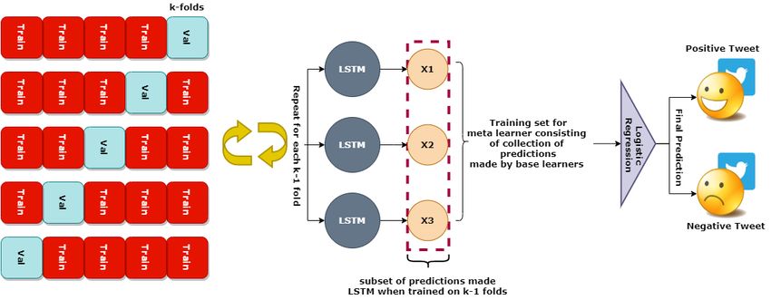
3.8. Proposed Framework of LR-LSTM Model
This study focuses on the sentiment classification of tweets by integrating a stacked
approach to construct an ensemble of LR and LSTM. Stacking is an ensemble of heteroge-
neous base learners and a meta learner which uses the output prediction of base learners as
an input and then produces final predictions [50]. Each base-learner is trained similarly as
k-fold cross-validation where each fold consisted of m/k number of training samples where
m is the number of total records in the dataset and k is the number of folds. Training of base
learners is carried out on k − 1 folds, whereas one-fold is used for validation. Base learners
produce n number of predictions for each instance of data for m-fold which results in an
m/k × n matrix. Afterwards, the meta learner is trained on this matrix and makes final
predictions. The proposed stacked ensemble model integrates 3 LSTMs as base-learners,
which will create individual predictions on the training data. These predictions will be
treated as training data for the meta learner. The architecture of the proposed LR-LSTM
model is shown in Figure 1.
Figure 1. Architecture of the proposed LR-LSTM model.
3.9. Proposed Methodology
This study aims at investigating the sentiment of tweets by integrating a lexical
dictionary along with a stacked ensemble model. Dataset “Sentiment140” is utilized for the
evaluation of the proposed approach. It consists of 1.6 million tweets among which 50%
are positive and 50% are negative tweets. The tweets in this study are reannotated using
TextBlob which resulted in positive and negative tweets which are further compared with
the original sentiments of the tweets. The comparison shows that TextBlob annotated the
tweets with more efficacy as compared to the original sentiment annotations. Afterward,
the data are preprocessed to transform the raw data into useful data by removing data
that are irrelevant for the sentiment analysis. Preprocessed data are then split into training
and testing sets with a 70:30 ratio. The proposed LR-LSTM model is then trained on the
training set and evaluated on the testing set in terms of accuracy, precision, recall, and
F1 Score. The proposed methodology is illustrated in Figure 2.Information 2021, 12, 374 10 of 19
Figure 2. Architecture of the proposed methodology.
3.10. Performance Evaluation Criteria
Evaluation parameters are used to evaluate the performance of models including preci-
sion, F1 Score, recall, and accuracy [51]. These are the commonly used evaluation metrics.
3.10.1. Accuracy
Accuracy is the measure of correctly predicted instances from total instances. It has
the highest value of 1 and lowest value of 0 and is calculated by the following formula:
Number o f correct predictions
Accuracy = (4)
Total number o f predictions
For binary classification, accuracy can be calculated as follows:
TP + TN
Accuracy = (5)
TP + TN + FP + FN
where FN, FP, TN, and TP show false negative, false positive, true negative, and true
positive are defined as follows [52]:
• False-negative (FN): Incorrectly predicted negative instances.
• False-positive (FP): Incorrectly predicted positive instances.
• True negative (TN): Correctly predicted negative instances.
• True Positive (TP): Correctly predicted positive instances.
3.10.2. Precision
Precision is the veracity of the predicting model. Precision refers to the percentage of
instances predicted as positive and that are actually positive. It can be computed as:
TP
Precision = (6)
TP + TN
3.10.3. Recall
A recall is the completeness of the classifier. It describes the percentage of correctly
predicted instances from the positive class. Recall can be computed by the following formula:
TP
Recall = (7)
TP + FNInformation 2021, 12, 374 11 of 19
3.10.4. F1 Score
F1 Score is the harmonic mean between precision and recall, in other words, F1 Score
conveys the balance between precision and recall. Like another score, it provides a float
value within the range of 0 and 1.
Precision ∗ Recall
F1 Score = (8)
Precision + Recall
4. Results and Analysis
This section contains detailed experimental results along with an analysis of the results.
A diverse range of experiments was conducted involving several ML models to evaluate the
performance of these models with three different feature extraction techniques including
BOW, TF-IDF, and BOW + TF-IDF. Experiments were conducted by integrating original
sentiments as well as sentiments extracted by TextBlob. The sole purpose of carrying out
a variety of experiments is to acquire the highest accuracy pertaining to the sentiment
classification of the sentiment140 dataset. In this section, we have compared our proposed
approach with previous studies conducted on the sentiment140 dataset.
4.1. Experimental Results of ML Models with Original Sentiment of the Sentiment140 Dataset
We first illustrate the experimental results of ML models trained on features extracted
by TF-IDF with original sentiments from the dataset, which are shown in Table 7. Statistical
model LR outperformed two other models in terms of evaluation metrics. It acquired the
highest accuracy of 0.75 when integrated with features extracted by TF-IDF with a precision
of 0.76, recall of 0.76, and of F1 Score 0.75, whereas the tree-based models such as ADB and
RF acquired 0.73 accuracies. RF yielded the lowest precision when analyzing sentiments of
the dataset by integrating TF-IDF features. From the results, it can be seen that, for original
sentiments and TF-IDF features, RF performed the worst. Conversely, it can be observed
that RF predicted a negative class with the highest precision of 0.77 and lowest recall of
0.70, whereas, in terms of positive class, LR remains the leading ML model with the highest
precision of 0.73 and lowest recall of 0.77.
Table 7. Experimental results of ML models with original sentiments using TF-IDF.
Classifier Accuracy Class Precision Recall F1 Score
LR 0.75 negative 0.76 0.72 0.73
positive 0.73 0.77 0.75
macro avg 0.76 0.76 0.75
ADB 0.73 negative 0.76 0.63 0.70
positive 0.69 0.82 0.75
macro avg 0.73 0.73 0.73
RF 0.73 negative 0.77 0.70 0.72
positive 0.69 0.82 0.75
macro avg 0.73 0.73 0.73
Similarly, with features extracted by BOW, LR yielded the highest accuracy of 0.74
along with the highest precision, recall, and F1 Score of 0.76, 0.75, and 0.75 as compared to
other ML models as shown in Table 8. This shows the effectiveness of LR in classifying the
sentiments of tweets. On the other hand, RF acquired the lowest accuracy of 0.73 and ADB
acquired 0.74 accuracy. Despite showing the highest accuracy, LR was not able to provide
optimized results in the prediction of the negative class, as RF leads with 0.78 precision
and lowest recall of 0.63. As for the positive class, LR outperformed other ML models with
the highest precision of 0.73 and the lowest recall of 0.78, although the F1 Score, which is
the harmonic mean of precision and recall, remains the same i.e., 0.75 in the prediction of
the positive class.Information 2021, 12, 374 12 of 19
Table 8. Experimental results of ML models with original sentiments using BOW.
Classifier Accuracy Class Precision Recall F1 Score
negative 0.77 0.71 0.74
LR 0.74 positive 0.73 0.78 0.75
macro avg 0.76 0.75 0.75
negative 0.78 0.65 0.72
ADB 0.74 positive 0.70 0.82 0.75
macro avg 0.74 0.72 0.73
negative 0.79 0.63 0.70
RF 0.73 positive 0.70 0.82 0.76
macro avg 0.71 0.70 0.70
In the case of the feature union, it can be observed that LR acquired the highest
accuracy score of 0.78 with 0.78 precision, 0.76 recall, and F1 Score as shown in Table 9.
The stable values of precision, recall, and F1 Score show the efficacy of LR when trained
with features extracted by the feature union. ADB on the contrary did not perform well,
whereas RF acquired an accuracy score of 0.76. In terms of the positive class, LR yielded
the highest precision, recall, and F1 Score of 0.78, 0.76, 0.76 respectively; in the case of the
negative class LR outperformed the other models.
Table 9. Experimental results of ML models with original sentiments using a feature union.
Classifier Accuracy Class Precision Recall F1 Score
negative 0.79 0.76 0.76
LR 0.78 positive 0.78 0.76 0.76
macro avg 0.78 0.76 0.76
negative 0.77 0.64 0.70
ADB 0.73 positive 0.71 0.84 0.74
macro avg 0.73 0.73 0.72
negative 0.78 0.76 0.73
RF 0.76 positive 0.75 0.75 0.77
macro avg 0.76 0.76 0.75
4.1.1. Comparative Analysis of ML Models with Original Sentiments Using TF-IDF, BOW
and BOW + TF-IDF
Figure 3 shows the comparison between the performance of ML models using three dif-
ferent feature extraction techniques when original sentiments of the dataset were integrated.
It can be observed that the feature union, i.e., BOW + TF-IDF boosted the performance
of LR. Moreover, a boost in the performance of ADB and RF can also be noted with the
feature union, showing that the features extracted by the union of BOW and TF-IDF are
more correlated with the target sentiments as compared to features extracted by BOW
and TF-IDF individually. It also creates a larger feature set for the models to train, thus
enhancing the performance of the models. On the contrary, models including RF and ADB
did not quite perform well with features extracted by TF-IDF, whereas the performance of
LR remained the same with TF-IDF and BOW.
4.1.2. Experimental Results of Proposed LR-LSTM with Original Sentiments
The performance of ML models varies with feature extraction techniques, thus leaving
room for improvement. To enhance the accuracy of sentiment classification of tweets,
this study proposes a stacked ensemble model LR-LSTM. The proposed model does not
require any feature extraction technique as LSTM is a deep learning approach that has the
capability of extracting features automatically. LR is trained on features extracted by LSTM.
The experimental results of the proposed LR-LSTM with original sentiments as the target
value are shown in Table 10. It can be observed that our proposed model outperformed the
conventional state-of-the-art models in terms of accuracy, precision, recall, and F1 Score.
Proposed LR-LSTM acquired a maximum accuracy of 0.81 which shows the effectiveness
of the proposed stacked ensemble model.Information 2021, 12, 374 13 of 19
Figure 3. Performance comparison of ML models using three different feature extraction techniques.
Table 10. Experimental results of LR-LSTM with original sentiments.
Accuracy Class Precision Recall F1 Score
negative 0.82 0.80 0.80
0.80 positive 0.81 0.81 0.80
Macro avg 0.81 0.80 0.90
4.2. Experimental Results of ML Models with TextBlob Sentiment
Table 11 shows that the highest accuracy score of 0.95 is yielded by LR through
integration when trained with features extracted by TF-IDF and given the sentiments
extracted by TextBlob. This shows that TextBlob sentiments are in more correlation with
the feature set extracted by TF-IDF. Similarly, an improvement in the performance of ML
models, including ADB and RF, shows the efficacy of using TextBlob sentiments. In terms
of positive class, LR yielded the highest precision and lowest recall as compared to other
ML models, whereas, in the case of the negative class, ADB is the leading ML model in
terms of the highest precision of 0.96. Overall, it can be observed that LR performed well
with TextBlob sentiments when trained on features extracted by TF-IDF.
Experiments conducted using features extracted by BOW with TextBlob sentiments
as target values resulted in comparatively better performance in the case of LR shown
in Table 12. Concerning the BOW features, LR outperformed the tree-based model RF
and boosting model ADB by achieving a 0.97 accuracy score. LR also performed well in
terms of other evaluation parameters. While ADB yielded an accuracy score of 0.92, RF
performed the worst with a 0.82 accuracy score.
Table 13 shows experimental results of ML models when trained on features extracted
by the feature union. The results showed that LR surpassed other ML models by achieving
an accuracy of 0.98 with similar precision, recall, and F1 Score.
Table 11. Experimental results of ML models with TextBlob sentiments using TF-IDF.
Model Accuracy Class Precision Recall F1 Score
negative 0.95 0.95 0.95
LR 0.95 positive 0.95 0.95 0.95
avg 0.95 0.95 0.95
negative 0.96 0.87 0.92
ADB 0.92 positive 0.89 0.97 0.93
avg 0.92 0.92 0.92
negative 0.95 0.74 0.83
RF 0.84 positive 0.79 0.96 0.87
avg 0.87 0.85 0.85Information 2021, 12, 374 14 of 19
Table 12. Experimental results of ML models with TextBlob sentiments using BOW.
Model Accuracy Class Precision Recall F1 Score
negative 0.97 0.98 0.98
LR 0.97 positive 0.97 0.98 0.97
avg 0.97 0.98 0.97
negative 0.97 0.87 0.92
ADB 0.92 positive 0.89 0.97 0.93
avg 0.93 0.92 0.92
negative 0.99 0.65 0.78
RF 0.82 positive 0.74 0.99 0.85
avg 0.87 0.82 0.82
Table 13. Experimental results of ML models with TextBlob sentiments using the feature union.
Model Accuracy Class Precision Recall F1 Score
negative 0.98 0.98 0.98
LR 0.98 positive 0.98 0.98 0.98
avg 0.98 0.98 0.98
negative 0.91 0.87 0.91
ADB 0.92 positive 0.88 0.97 0.92
avg 0.90 0.92 0.92
negative 0.98 0.73 0.84
RF 0.86 positive 0.78 0.99 0.88
avg 0.88 0.86 0.86
4.2.1. Comparative Analysis of ML Models with TextBlob Sentiments Using TF-IDF, BOW
and BOW + TF-IDF
Figure 4 shows that the highest accuracy is achieved by LR with BOW + TF-IDF using
TextBlob sentiments, while the performance of ADB remained the same with three feature
extraction techniques. BOW + TF-IDF creates a large feature set for the models to train,
thus resulting in better performance of models. On the other hand, RF performed poorly
in comparison to the other two ML models. From this, we can observe that LR, due to its
statistical structure, transcended in classifying sentiments of tweets. LR not only quantifies
the coefficient size but also provides the direction of association (negative or positive) of
the record under analysis. This makes LR more efficient as compared to other ML models
in this study.
Figure 4. Performance comparison of ML models using three different feature extraction techniques.
4.2.2. Experimental Results of Proposed LR-LSTM with TextBlob Sentiments
Stacking is a powerful solution for combining the learning models. From the above
discussion, it can be observed that LR with its efficacy has surpassed other ML models in
classifying sentiments of tweets. This provides the basis of our proposed model LR-LSTM.
LSTM works well with long time dependencies, giving us an edge in experimental results.Information 2021, 12, 374 15 of 19
From Table 14, it can be observed that our proposed model LR-LSTM achieved state-of-the-
art results by classifying sentiments of tweets extracted by TextBlob. LR-LSTM does not
require extraction of features separately and thus it is a time-efficient method. It acquired
an accuracy of 0.99 with similar precision, recall, and F1 Score showing the robustness and
effectiveness of the proposed model.
Table 14. Experimental results of LR-LSTM with TextBlob sentiments.
Accuracy Class Precision Recall F1 Score
negative 0.99 0.99 0.98
0.99 positive 0.99 0.98 0.99
Macro avg 0.99 0.99 0.99
4.3. Impact of TextBlob Sentiments on Classifiers
Experimental results illustrated that the classifier efficiently predicted sentiments of
tweets extracted by TextBlob. LR performed well with its capability of predicting model
coefficients as a measure of feature importance. On the contrary, its performance was
limited with original sentiments as the target value. This shows that TextBlob annotates
the tweets which are more correlated with its textual features. This shows the effectiveness
of the proposed methodology. ADB also performed comparatively better, but its sensitivity
to outliners limited its performance as compared to LR. RF performed poorly due to its
continuous approximation, but its performance was boosted with TextBlob sentiments.
On the other hand, our proposed LR-LSTM showed empirical results with the highest
accuracy score of 0.99 which is an optimized accuracy score showing the robustness of the
proposed model.
From Figure 5 it can be observed that performance of all classifiers was enhanced
with the sentiments extracted by TextBlob, as compared to their performance with the
original sentiments. This shows that sentiments labeled by TextBlob are more relevant
to the features of the tweets. TextBlob assigns a sentiment score to words with greater
clarification in relation to its PatternAnalyzer property, which results in better learning for
the classifiers and hence better performance.
Figure 5. Accuracy score of classifiers with TextBlob sentiments and original sentiments (LR + TF-IDF
refers to an LR model trained on features extracted by TF-IDF; the same goes for other labels).
4.4. Comparative Analysis of Proposed LR-LSTM with Deep Learning Models
The performance of the proposed LR-LSTM model was compared with several deep
learning models including the gated recurrent unit (GRU), convolutional neural network
(CNN), and long short-term memory (LSTM) to validate the effectiveness of the model.
GRU is a modified version of a recurrent neural network (RNN) which deals with the
problem of the vanishing gradient of a standard RNN. CNN, on the other hand, has
the ability to extract the textual features from the input data in a direct manner withoutInformation 2021, 12, 374 16 of 19
the requirement of preprocessing tasks. CNN has three main components including a
convolution layer, pooling layer, and dense layer to carry out predictive tasks. LSTM
makes a prediction based on individual time steps of the sequential data. Considering the
aforementioned structures of CNN and LSTM, we also employed a combined CNN–LSTM
model. Hyperparameter settings for each deep learning model are presented in Table 15.
Table 15. Deep Learning Models’ Hyperparameter Settings.
Models Hyperparameter Settings
embedding=5000, dropout=0.5, dense_layer=3, activation=’softmax’, loss=’categorical_crossentropy’, optimizer=’adam’,
LSTM
epoch=100, batch_size=16, LSTM(100)
embedding=5000, dropout=0.5, dense_layer=3, activation=’softmax’, loss=’categorical_crossentropy’, optimizer=’adam’,
GRU
epoch=100, batch_size=16, GRU(256), SimpleRNN(128)
embedding=5000, dropout=0.5, dense_layer=3, activation=’softmax’, loss=’categorical_crossentropy’, optimizer=’adam’,
CNN
epoch=100, batch_size=16, Conv1D(128, 5, activation=’relu’), MaxPooling1D(pool_size=4)
embedding=5000, dropout=0.5, dense_layer=3, activation=’softmax’, loss=’categorical_crossentropy’, optimizer=’adam’,
CNN-LSTM
epoch=100, batch_size=16, Conv1D(128, 5, activation=’relu’), MaxPooling1D(pool_size=4), LSTM(100)
Extensive experiments were conducted using the sentiment140 dataset combined with
TextBlob sentiments for the training and testing of the deep learning models. Experimental
results reveal that performance of the deep learning models is comparatively lower than the
proposed LR-LSTM classifier which shows the effectiveness of this study. Table 16 presents
the performances of deep learning models in comparison with the proposed approach. The
results disclose that the highest accuracy score of 0.96 is achieved by LSTM as compared to
other deep learning models. This analysis also supports the integration of LSTM as a base
learner in the proposed LR-LSTM model.
Table 16. Experimental results of Deep learning models using TextBlob sentiments.
Classifiers Accuracy Precision Recall F1 Score
GRU 0.95 0.95 0.95 0.95
LSTM 0.96 0.96 0.96 0.96
CNN 0.93 0.93 0.93 0.93
CNN–LSTM 0.93 0.93 0.93 0.93
4.5. Comparative Analysis of Proposed Study with Correlated Studies
A considerable amount of research has been carried out on the benchmark senti-
ment140 dataset. In this section, we compare our proposed approach to a few state-of-the-
art approaches proposed in previous studies to carry out sentiment classification of tweets
in the sentimnet140 dataset. Previous studies are summarized in Table 17 which shows that
our proposed system exceeded in performance in comparison to previous studies which
shows the potency of our proposed approach.
Table 17. Comparative Analysis of the Proposed Study with Correlated Studies.
Ref Year Proposed Methodology Classifier with Highest Accuracy Accuracy
Analyzed the impact of various features such as combining bigram
features with unigrams, unigrams and word features without
NB with unigram and bigram
[53] 2018 stopwords, bigrams with word features without stopwords, and the 88%
features.
highest weighted unigrams with the highest weighted bigrams, on
the performance of ML classifiers.
Calculating sentiment score of a tweet and then classifying based on
[22] 2018 its sentiment score with a majority voting ensemble model provides Ensemble of NB, RF, LR and SVM 75.81%
comparatively better results.
An ensemble of two ML models can perform comparatively better
[54] 2018 in classifying sentiments of tweets as comparison to individual LR-SVM 81.83%
classifiers.
Deep learning models perform better with word embedding in
[55] 2020 RNN with word Embedding 82.8%
comparison to TF-IDF features.
Sentiments extracted by lexical dictionary are more correlated with
Proposed 2021 the textual features, thus enhancing the performance of a stacked LR-LSTM 99%
ensemble model.Information 2021, 12, 374 17 of 19
5. Conclusions
This study proposes a novel approach by integrating a lexical dictionary along with a
stacked ensemble of three LSTMs and LR which is aimed at enhancing the performance
of sentiment analysis of tweets from the sentiment140 dataset. The study suggests that
sentiments extracted from TextBlob are in more correlated with the textual features of
tweets as compared to the original sentiments. Training of classifiers was carried out on
a 70% training set and tested on a 30% testing set. No feature extraction was required
in terms of our proposed approach, contrarily, ML models including RF, LR, and ADB
required extracted features for which three feature extraction techniques including BOW,
TF-IDF, and BOW + TF-IDF were used. Classification of tweets is performed using the
proposed model and above-mentioned ML classifiers with original sentiments and TextBlob
sentiments. Conventional ML models revealed scant performance in classifying sentiments
of tweets given the original sentiments, but their performance enhanced with TextBlob
sentiments, thus revealing that there is a high level of association between tweets and
sentiments extracted by TextBlob as compared to the original sentiments. The proposed
LR-LSTM model is adapted for optimized results which outperformed other conventional
models with a maximum accuracy of 99%, precision of 99%, recall of 99%, and F1 Score of
99%, respectively, which shows the efficacy and feasibility of the proposed model.
Modification of the proposed LR-LSTM model can be a future direction. Furthermore,
preprocessing techniques including POS tagging can further improve the accuracy of the
model. Moreover, this research can be extended to sarcasm detection, fake review detection,
fake advertisement classification, spam email detection, and many more. Additionally,
word embeddings can be added to the model.
Author Contributions: Conceptualization, B.G. and A.W.; data curation, B.G. and A.W.; formal anal-
ysis, B.G. and D.Z.; funding acquisition, A.W.; investigation, D.Z., D.Z. and A.W.; methodology, B.G.,
A.W. and D.Z.; project administration, B.G.; resources, A.W.; software, B.G. and D.Z.; supervision,
D.Z.; visualization, D.Z.; writing—original draft, B.G.; writing—review and editing, A.W. All authors
have read and agreed to the published version of the manuscript.
Funding: This research received no external funding.
Institutional Review Board Statement: Not applicable.
Informed Consent Statement: Not applicable.
Data Availability Statement: Not applicable.
Conflicts of Interest: The authors declare no conflict of interest.
References
1. Statista. Available online: https://www.statista.com/statistics/346167/facebook-global-dau/ (accessed on 6 September 2021).
2. Statista. Available online: https://www.statista.com/statistics/272014/global-social-networks- (accessed on 6 September 2021).
3. You, Q.; Bhatia, S.; Luo, J. A picture tells a thousand words—About you! User interest profiling from user generated visual
content. Signal Process. 2016, 124, 45–53. [CrossRef]
4. Persia, F.; D’Auria, D. A survey of online social networks: Challenges and opportunities. In Proceedings of the 2017 IEEE
International Conference on Information Reuse and Integration (IRI), San Diego, CA, USA, 4–6 August 2017; pp. 614–620.
5. Khattak, A.M.; Batool, R.; Satti, F.A.; Hussain, J.; Khan, W.A.; Khan, A.M.; Hayat, B. Tweets classification and sentiment analysis
for personalized tweets recommendation. Complexity 2020, 2020, 8892552. [CrossRef]
6. Crisci, A.; Grasso, V.; Nesi, P.; Pantaleo, G.; Paoli, I.; Zaza, I. Predicting TV programme audience by using twitter based metrics.
Multimed. Tools Appl. 2018, 77, 12203–12232. [CrossRef]
7. McConnell, J. Twitter and the 2016 US Presidential Campaign: A Rhetorical Analysis of Tweets and Media Coverage. Master’s
Thesis, New York University, New York, NY, USA, 2015.
8. Coletta, L.F.; da Silva, N.F.; Hruschka, E.R.; Hruschka, E.R. Combining classification and clustering for tweet sentiment analysis.
In Proceedings of the 2014 Brazilian Conference on Intelligent Systems, Sao Paulo, Brazil, 18–22 October 2014; pp. 210–215.
9. Dhelim, S.; Ning, H.; Aung, N.; Huang, R.; Ma, J. Personality-Aware Product Recommendation System Based on User Interests
Mining and Metapath Discovery. IEEE Trans. Comput. Soc. Syst. 2020, 8, 86–98. [CrossRef]
10. Cambria, E.; Das, D.; Bandyopadhyay, S.; Feraco, A. Affective computing and sentiment analysis. In A Practical Guide to Sentiment
Analysis; Springer: Berlin, Germany, 2017; pp. 1–10.You can also read