Pruning deep neural networks generates a sparse, bio-inspired nonlinear controller for insect flight
←
→
Page content transcription
If your browser does not render page correctly, please read the page content below
Pruning deep neural networks generates a sparse,
                                                        bio-inspired nonlinear controller for insect flight
                                                        Olivia Zahn 1 , Jorge Bustamante, Jr.2 , Callin Switzer2 , Thomas Daniel2 , J. Nathan
                                                        Kutz3 ,

                                                        1 Department of Physics, University of Washington, Seattle, WA USA
                                                        2 Department of Biology, University of Washington, Seattle, WA USA
arXiv:2201.01852v1 [q-bio.QM] 5 Jan 2022

                                                        3 Department of Applied Mathematics, University of Washington, Seattle, WA USA

                                                        Abstract
                                                        Insect flight is a strongly nonlinear and actuated dynamical system. As such, strategies
                                                        for understanding its control have typically relied on either model-based methods or
                                                        linearizations thereof. Here we develop a framework that combines model predictive
                                                        control on an established flight dynamics model and deep neural networks (DNN) to
                                                        create an efficient method for solving the inverse problem of flight control. We turn to
                                                        natural systems for inspiration since they inherently demonstrate network pruning with
                                                        the consequence of yielding more efficient networks for a specific set of tasks. This
                                                        bio-inspired approach allows us to leverage network pruning to optimally sparsify a
                                                        DNN architecture in order to perform flight tasks with as few neural connections as
                                                        possible, however, there are limits to sparsification. Specifically, as the number of
                                                        connections falls below a critical threshold, flight performance drops considerably. We
                                                        develop sparsification paradigms and explore their limits for control tasks. Monte Carlo
                                                        simulations also quantify the statistical distribution of network weights during pruning
                                                        given initial random weights of the DNNs. We demonstrate that on average, the
                                                        network can be pruned to retain approximately 7% of the original network weights, with
                                                        statistical distributions quantified at each layer of the network. Overall, this work shows
                                                        that sparsely connected DNNs are capable of predicting the forces required to follow
                                                        flight trajectories. Additionally, sparsification has sharp performance limits.

                                                        Author summary
                                                        Originally inspired by biological nervous systems, deep neural networks (DNNs) are
                                                        powerful computational tools for modeling complex systems. DNNs are used in a
                                                        diversity of domains and have helped solve some of the most intractable problems in
                                                        physics, biology, and computer science. Despite their prevalence, the use of DNNs as a
                                                        modeling tool comes with some major downsides. DNNs are highly overparameterized,
                                                        which often results in them being difficult to generalize and interpret, as well as being
                                                        incredibly computationally expensive. Unlike DNNs, which are often trained until they
                                                        reach the highest accuracy possible, biological networks have to balance performance
                                                        with robustness to a noisy and dynamic environment. Biological neural systems use a
                                                        variety of mechanisms to promote specialized and efficient pathways capable of
                                                        performing complex tasks in the presence of noise. One such mechanism, synaptic
                                                        pruning, plays a significant role in refining task-specific behaviors. Synaptic pruning
                                                        results in a more sparsely connected network that can still perform complex cognitive

                                      January 7, 2022                                                                                         1/22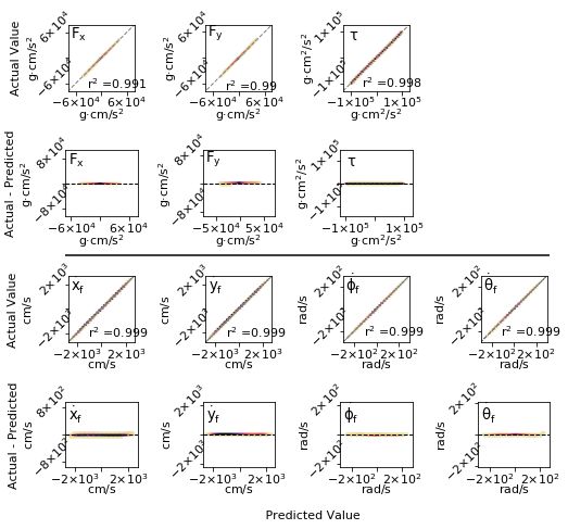
and motor tasks. Here, we draw inspiration from biology and use DNNs and the
                  method of neural network pruning to find a sparse computational model for controlling
                  a biological motor task.

                  Introduction
                  Between childhood and adolescence, the number of synaptic connections between
                  neurons sharply decreases through a process called synaptic pruning [1]. Depending on
                  the neural system, synaptic pruning can improve the brain’s efficiency and affect
                  cognitive function. In fact, synaptic pruning is seen as a mechanism for learning, in
                  which the environment affects which neural connections are maintained and which are
                  removed [2]. Refinement of neural connections via pruning occurs in wide ranging taxa,
                  from humans to Drosophila and in systems ranging from sensory input to motor
                  control [3, 4]. For example, during metamorphosis of the hawkmoth, Manduca Sexta,
                  synapses are pruned and reconnected to enable adult-specific behaviors [5]. Synaptic
                  pruning plays a significant role in refining task-specific behaviors, the result of which is
                  a more sparsely connected network that can still perform complex cognitive and motor
                  tasks.
                      There is a rich basis of literature in biological synaptic pruning. However, the main
                  finding across these numerous studies is that synaptic pruning plays a major role in the
                  refinement of neural connectivity [3]. Through the overgrowth of synapses and their
                  subsequent pruning, biological neural systems are made both optimal for a specific task
                  and more efficient for having more sparse connectivity. Deep neural networks (DNNs),
                  which were originally motivated by the visual cortex of cats and the pioneering work of
                  Hubel and Wiesel [6, 7], are often considered as mathematical proxies for biological
                  neural processing. The universal approximation properties of DNNs [8] make them ideal
                  for modeling high-dimensional, complex, nonlinear mappings for a large diversity of
                  problems. From image and speech recognition [9, 10] to fluid flow control [11, 12], DNNs
                  learn input-to-output mappings by combining gradient descent with the
                  backpropagation algorithm. Like biological pruning, DNNs have an extensive literature
                  dedicated to improving the generalization capabilities (i.e. performance on unseen data)
                  and computational efficiency of DNNs through the mechanism of pruning.
                      The sparsification of such DNNs has typically been motivated by the pernicious
                  effects of over-fitting data, and to a lesser extent, the DNNs computational and memory
                  footprint, i.e. the need to be implemented on small portable devices such as smart
                  phones. Dropout, for instance, was one of the early versions of sparsification that
                  allowed for greater generalization capabilities [10, 13, 14]. However, standard dropout
                  methods typically only enforce temporary sparsification since the algorithm often allows
                  for nodes to again re-train their weights from their zeroed-out state. Thus most DNNs
                  typically remain highly over-parameterized and their layers are fully-connected. For
                  example, the natural language processing model, GPT-3, is the largest DNN ever built
                  with 175 billion parameters [15], and successful models with millions of parameters are
                  not uncommon. There are many different methods to make DNNs more sparse, ranging
                  from regularization during training [16] to specifying sparse architectures [17].
                  Biologically inspired neural network pruning has also been shown to be an effective
                  method for sparsifying a DNN without compromising performance [18–22]. In neural
                  network pruning, the connectivity of a DNN is made more sparse by forcing select
                  weights between the layers to zero and then retraining, resulting in a more sparse
                  network that is capable of performing comparably to the fully-connected network up to
                  a certain limit. Pruning has been used to prevent network overfitting and to reduce
                  overall model size. Pruned DNNs have the advantage of (i) having a small memory
                  footprint, (ii) providing improved generalization, and (iii) being more efficient for

January 7, 2022                                                                                         2/22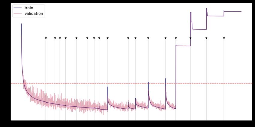
generating input-output computations. Thus they have important practical advantages
                  over their fully-connected counterparts. They are also more representative of biological
                  neural systems, in which neural pathways are sparsely and specifically connected for
                  task performance.
                      The inverse problem of insect flight is a highly nonlinear dynamical system, in part
                  due to the unsteady mechanisms of flapping flight [23, 24] and the noisy environment
                  through which insects maneuver. As such, the inverse problem of insect flight serves as
                  an exemplar to study whether a DNN can solve a biological motion control problem
                  while maintaining a sparse connectivity pattern. In an inverse problem, the initial and
                  final conditions of a dynamical system are known and used to find the parameters
                  necessary to control the system. In other words, the DNN in this study is trained to
                  predict the controls required to move the simulated insect from one state space to
                  another. Solving the inverse problem of insect flight has been previously simulated using
                  a genetic algorithm wedded with a simplex optimizer for hawkmoth level forward flight
                  and hovering [25]. Another study linearized the dynamical system of simulated
                  hawkmoth flight and found the system to operate on the edge of stability [26]. Recently,
                  a study developed an inertial dynamics model of M. sexta flight as it tracked a
                  vertically oscillating signal, which modeled the control inputs using Monte Carlo
                  methods in a model-inspired by model predictive control (MPC) [27].
                      In this work, we use the inertial dynamics model in [27] to simulate examples of M.
                  sexta hovering flight. Fig. 1 shows the physical parameters of the simulated moth and
                  the inertial dynamics model. These data are used to train a DNN to learn the
                  controllers for hovering. Drawing inspiration from pruning in biological neural systems,
                  we sparsify the network using neural network pruning. Here, we prune weights based
                  simply on their magnitudes, removing those weights closest to zero. Importantly, the
                  pruned weights remain zeroed out throughout the sparsification process. This
                  bio-inspired approach to sparsity allows us to find the optimally sparse network for
                  completing flight tasks. Insects must maneuver through high noise environments to
                  accomplish controlled flight. It is often assumed that there is a trade-off between perfect
                  flight control and robustness to noise and that the sensory data may be limited by the
                  signal-to-noise ratio. Thus the network need not train for the most accurate model since
                  in practice noise prevents high-fidelity models from exhibiting their underlying accuracy.
                  Rather, we seek to find the sparsest model capable of performing the task given the
                  noisy environment. We employed two methods for neural network pruning: either
                  through manually setting weights to zero or by utilizing binary masking layers.
                  Furthermore, the DNN is pruned sequentially, meaning groups of weights are removed
                  slowly from the network, with retraining in-between successive prunes, until a target
                  sparsity is reached. Monte Carlo simulations are also used to quantify the statistical
                  distribution of network weights during pruning given random initialization of network
                  weights. This work shows that sparse DNNs are capable of predicting the controls
                  required for a simulated hawkmoth to move from one state-space to another, or through
                  a sequence of control actions. Specifically, for a given signal-to-noise level the pruned
                  network can perform at the level of the fully connected network while requiring only a
                  fraction of the memory footprint and computational power.

                  Results
                  Network pruning results
                  Fig. 2 shows the learning curve for a network trained using the sequential pruning
                  protocol with TensorFlow’s Model Optimization Toolkit (see Methods section for
                  details) [28]. The network is trained until a minimum error is reached, and then pruned

January 7, 2022                                                                                        3/22
(A) Schematic of simulated moth
(B) Simulated moth data generation
Time
Initial conditions Final conditions
Dynamics
(ODEs)
20 ms
Biomechanical parameters
Inertial Aerodynamic
Randomized torques
and forces
(C) Neural network inverse model
Pruning
Fig 1. Inverse problem of flight control. (A) The moth body is made of two
ellipses attached with a spring. There are three control variables (F , α, and τ ) and four
parameters to describe the state space (x, y, θ, and φ). See Table 2 and 3 for a full
description of model parameters. (B) The differential equation solver solves the forward
problem of insect flight control. (C) The neural network is an attempt to solve the
inverse problem of flight control.
to a specified sparsity percentage and then retrained until the loss is once again
minimized. The sparsity (or pruning) percentages are shown in Fig. 2 where they occur
in the training process. An arbitrary threshold error of 10−3 (shown as a red, dashed
line) was chosen to define the optimally sparse network (i.e. sparsest possible network
that performs under the specified loss). This specific threshold value was chosen
because it is near the performance of the trained, fully-connected network. In practice,
the red line represents the noise level encountered in the flight system. Specifically,
given a prescribed signal-to-noise ratio, we wish to train a DNN to accomplish a task
with a certain accuracy that is limited by noise. Thus high-fidelity models, which can
only practically exist with perfect data, are traded for sparse models which are capable
of performing at the same level for a given noise figure. In the example in Fig. 2, the
optimally sparse network occurs at 94% sparsity (or when only 6% of the connections
remain). Beyond 94% sparsity, the performance of the network breaks down because too
many critical weights have been removed.
January 7, 2022 4/22train
validation
Mean-squared loss
Epoch
Fig 2. Learning curve for sequential pruning of network. Fully-connected
neural network is trained until the mean-squared error is minimized. Then, the network
is sequentially pruned by adding in masking layers and trained again. The performance
of the network improves below the minimum error achieved by the fully-connected
network for low levels of pruning, but performs comparably to the fully-connected
network until 94% of the network is pruned.
Monte Carlo results
To compare the effects of pruning across networks, we trained and pruned 1320
networks with different random initializations on the same dataset. In this experiment,
the hyper-parameters, pruning percentages, and architecture are held constant. Fig. 3
shows the training curves of 9 sample networks. The red, dashed line in each of the
panels represents the same threshold as in Fig. 2 (10−3 ). The black, solid lines in Fig. 3
represent the optimally sparse networks. Although the majority of networks in this
subset breakdown at 93% sparsity, a few breakdown at higher and lower levels of
connectivity.
Fig. 4 shows the loss after pruning the 1320 networks at varying pruning percentages
(from 0% sparsity to 98% sparsity). The box plot in Fig. 4 is directly comparable to Fig.
2, but it is the compilation of the results for many different networks. The networks do
not all converge to the same set of weights, which is evident by the numerous outliers,
as well as the variance around the median loss.
The median minimum loss achieved by the networks before pruning is 7.9 x 10⁻⁴ .
The first box in the box plot in Fig. 4 corresponds to the losses of all the trained
networks before any pruning occurs. The variance on the loss is relatively small, but
there are several outliers. Once again, the red, dashed line in the box plot in Fig. 4
represents the threshold below which a network is optimally sparse. Many networks
follow a similar pattern and perform under the threshold until they exceed 93% sparsity.
Also, many networks perform better than the median performance of the
fully-connected networks when pruned up to 85% sparsity.
The number of optimally sparse networks in each sparsity category is shown in the
bar plot at the top of Fig. 4. Of the 1320 networks trained, 858 of the networks are
optimally sparse at 93% sparsity. A small number of networks (5) remain under the
threshold up to 95% pruned. Note that the total number of networks represented in the
bar plot does not add up to 1320. This is because several networks never perform below
January 7, 2022 5/22Mean-squared loss
Batches
Fig 3. Performance breakdown of 9 sample pruned networks. The networks
are sequentially pruned. Each network is evaluated to find the optimally sparse network.
The red dashed line represents the performance threshold (10−3 ). The sparsest network
that performs below this threshold is shown by the solid, black vertical line.
the threshold throughout the sequential pruning process (see outliers in Fig. 4).
Analysis of layer sparsity
The subset of optimally sparse networks pruned to 93% is used in the following analysis
of network structure (858 networks). The sparsity across all the layers was found to be
uniform (7% of weights remain in each layer) despite not explicitly requiring uniform
pruning in the protocol. Table 1 shows the average number of remaining connections
across the 858 networks, as well as the variance and the fraction of remaining
connections.
Fig. 5 shows a box plot of the number of connections from the input layer to the
first hidden layer for the subset of pruned networks. Interestingly, the initial
head-thorax angular velocity was completely pruned out of all of the networks in the
subset, meaning it has no impact on the output and predictive power of the network.
Additionally, the initial abdomen angular velocity connects to either zero, one, or two
nodes in the second hidden layer, while all the other inputs have a median connection to
January 7, 2022 6/22Number of optimally
sparse networks
Mean-squared loss
Network sparsity
Fig 4. Monte Carlo analysis of pruned networks. 1320 networks are sequentially
pruned and loss of the pruned networks at each sparsity percentage is recorded in the
box plot. The bar plot records the number of networks that make it to the
corresponding sparsity percentage before exceeding the hypothetical threshold (10−3 ).
at least 5% of the weights in the first hidden layer.
Materials and methods
All code associated with the simulations and the DNNs is available on Github [29].
Moth model
The simulated insect uses an inertial dynamics model developed in Bustamante et al.,
2021 [27] and was inspired by hawkmoth flight control, M. sexta with body proportions
rounded to the nearest 0.1 cm. The simulated moth was made up of two ellipsoid body
segments, the head-thorax mass (m1 ) and the abdomen mass (m2 ). The body segments
are connected by a pin joint consisting of a torsional spring and a torsional damper as
seen in [30]. The simulated moth model could translate in x-y plane, and both the
head-thorax mass, and the abdominal mass could rotate with angles (θ,φ) in the x-y
plane . See Fig. 1 and Tables 2 and 3 for more description of the simulated insect.
The computational model of the moth had three control variables and four
state-space variables (as well as the respective state-space derivatives). This model is by
definition underactuated because the number of control variables is less than the
degrees of freedom. The controls are as follows: F , the magnitude of force applied; α
the direction of force applied (with respect to the midline of the head-thorax mass); and
January 7, 2022 7/22Table 1. Number of remaining parameters in networks pruned to 93%
sparsity This table gives the average number of remaining weights in each layer of the
networks pruned to 93% sparsity. The variance on the number of connections, as well as
the fraction of remaining connections are also given.
Layer i Average number remaining Variance Percentage remaining
1 280 23 0.07
2 11199 0 0.07
3 11199 0 0.07
4 447 0.04 0.07
5 8 6 0.07
Percent of remaining connections
Input parameter
Fig 5. Sparsity of input layer of networks pruned to 93% sparsity. Each box
represents the number of connections remaining between a parameter in the input layer
and the first hidden layer. For all 858 networks in this group, θ̇i was pruned entirely
from the network.
τ , the abdominal torque exerted about the pin joint connecting the two body segment
masses (with its equal and opposite response torque). The controls are randomized
every 20 ms, which is approximately the period of the wing downstroke or upstroke for
M. sexta (25 Hz wing beat frequency) [31].
The motion of the moth state-space is described by four parameters (x: horizontal
position, y: vertical position, θ: head-thorax angle, and φ: abdomen angle), as well as
the respective state-space derivatives (ẋ: horizontal velocity, ẏ: vertical velocity, θ̇:
head-thorax angular velocity, and φ̇: abdomen angular velocity). The x and y position
indicate the position of the pin joint where the head-thorax connects with the abdomen.
Generating training data
We used the ordinary differential equations from [27] (See Appendix, Equations 30-33)
to generate a dataset for training the deep neural network. All simulated trajectories
were started from the origin (i.e., (x0 ,y0 ) = (0,0)). We randomly sampled initial
January 7, 2022 8/22Vertical position (cm)
0.0 5
5
−2.5
0
0
−5.0
−5 0 −5 0 5 −5 0 5
Horizontal position (cm)
Fig 6. Example trajectories of the simulated insects. Each trajectory is 20 ms,
and each starts at (x,y) = (0,0). Force (F ) is indicated with the straight red arrow, and
torque (τ ) is shown with the curved arrows at the thorax-abdomen joint (red dot). The
center of mass of each body segment is shown with black dots.
horizontal velocity (ẋ0 ), vertical velocity (ẏ0 ), head-thorax angle (θ0 ), abdomen angle
(φ0 ), head-thorax angular velocity (θ̇0 ), and abdomen angular velocity (φ̇0 ) as shown in
Table 4. We also randomly sampled force (F ), force angle (α), and torque (τ ) as shown
in Table 4. The training dataset is comprised of 10 million simulated trajectories and
the test set contains an additional 5 million trajectories. The trajectories were
simulated using the Python (Python Software Foundation, https://www.python.org/)
function, scipy.integrate.odeint [32]. Fig. 1 shows which variables were inputs and
outputs from the differential equation solver.
Data preparation for deep neural network training
The force (F ) and force angle (α) were converted to horizontal and vertical components
(Fx and Fy ), using the following equations: Fx = F · cos(α) and Fy = F · sin(α). The
data were split into training and validation sets for cross validation (80:20 split). The
validation data is a sample used to provide an unbiased evaluation of a model fit while
tuning the hyper parameters (such as number of hidden units, number of layers,
optimizer, etc.). The data were scaled using a min-max scaler according to the training
dataset and transformed values to be between −0.5 and +0.5. The same scaler was then
used to transform the validation and test data.
Training and pruning a deep neural network
The deep, fully-connected neural network was constructed with ten input variables and
seven output variables (see Fig. 1). The initial and final state space conditions are the
inputs to the network: (ẋi , ẏi , φi , θi , φ̇i , θ̇i , xf , yf , φf , θf ). The network predicts the
control variables and the final derivatives of the state space in its output layer
(Fx , Fy , τ, ẋf , ẏf , φ̇f θ̇f ). The final derivatives of the state space were made outputs to
be able to chain together 20 ms solutions to allow the moth to complete a complex
trajectory for use in future work. The training and pruning protocols were developed
using Keras [33] with the TensorFlow backend [28]. To scale up training for the
statistical analysis of many networks, the training and pruning protocols were
parallelized using the Jax framework [34].
To demonstrate the effects of pruning, the network was chosen to have a deep,
feed-forward architecture with wide hidden layers (many more nodes than in the input
and output layer). The network had four hidden layers with 400, 400, 400, and 16 nodes,
respectively. Wide hidden layers were used rather than using a bottleneck structure
(narrower hidden layer width) to allow the network to find the optimal mapping with
little constraint, however, the specific choices of layer widths were arbitrary. The inverse
January 7, 2022 9/22Algorithm 1: Sequential pruning and fine-tuning
Train fully-connected model until loss is minimized;
Define list of sparsity percentages;
for Each sparsity percentage do
while Loss is not minimized do
for Each epoch do
Set n weights to zero s.t. n/N equals the sparsity percentage;
Evaluate loss;
Update weights;
end
end
end
tangent activation function was used for all hidden layers to introduce nonlinearity in
the model. To account for the multiple outputs, the loss function was the
uniformly-weighted average of the mean squared error for all the outputs combined.
m
1 X
M SE = yi − ŷi (1)
m i=1
For optimizing performance, there are several hyper-parameter differences in the
TensorFlow model and the Jax model. In developing the training and pruning protocol
in TensorFlow, the network was trained using the rmsprop optimizer with a batch size
of 212 samples. However, to scale up and speed up training we used the Jax framework,
the Adam optimizer [35], and the batch size was reduced to 128 samples. Regularization
techniques such as weight regularization, batch normalization, or dropout were not used.
However, early stopping (with a minimum delta of 0.01 with a patience of 1000 batches)
was used to reduce overfitting by monitoring the mean squared error.
After the fully-connected network is trained to a minimum error, we used the method
of neural network pruning to promote sparsity between the network layers. In this work,
a target sparsity (percentage of pruned network weights) is specified and those weights
are forced to zero. The network is then retrained until a minimum error is reached.
This process is repeated until most of the weights have been pruned from the network.
We developed two methods to prune the neural network: 1) a manual method that
involves setting a number of weights to zero after each training epoch and 2) a method
using TensorFlow’s Model Optimization Toolkit [28] which involves creating a masking
layer to control sparsity in the network. Both methods are described in detail in the
following sections.
Manual Pruning
Alg. 1 describes the a method of pruning in which the n weights whose magnitudes are
closest to zero are manually set to zero. If N is the total number of weights in the
network, the n weights are chosen such that n/N is equivalent to a specified pruning
percentage (e.g. 15%, 25%, ..., 98%). After the n weights are set to zero, the network is
retrained for one epoch. This process is repeated until the loss is minimized. After the
network has been trained to a minimum loss, we select the next pruning percentage from
the predetermined list and repeat the retraining process. The entire pruning process is
repeated until the network has been pruned to the final pruning percentage in the list.
Upon retraining, the weights are able to regain a non-zero weight and the network is
evaluated using these non-zero weights. Although this likely still captures the effects of
January 7, 2022 10/22Algorithm 2: Sequential pruning with masks and fine-tuning
Train fully-connected model until loss is minimized;
Define list of sparsity percentages;
for Each sparsity percentage do
Define pruning schedule using ConstantSparsity;
Create prunable model by calling prune low magnitude;
Train pruned model until loss is minimized;
end
pruning the network over the full training time, it is not true pruning in the sense that
connections that have been pruned can regain weight.
Pruning using Model Optimization Toolkit
The manual pruning method described above has the downside of allowing weights to
regain non-zero value after training. These weights are subsequently set back to zero on
the next epoch, but the algorithm does not guarantee that the same weights will be
pruned every time.
To ensure weights remain pruned during retraining, we implemented the pruning
functionality of a TensorFlow built toolkit called the Model Optimization Toolkit [28].
The toolkit contains functions for pruning deep neural networks. In the Model
Optimization Toolkit, pruning is achieved through the use of binary masking layers that
are multiplied element-wise to each weight matrix in the network. A four-layer neural
network can be mathematically described the following way.
ŷ = σ4 (A4 ...(σ1 (A1 x)) (2)
In Eq. 2, the inputs to the network are represented by x, the predictions by ŷ, the
weight matrices by Ai , and the activation function by σi , where i = 1, 2, 3, 4 for the four
layers of the network. During pruning, the binary masking matrix, Mi is placed
between each layer.
ŷ = M4 ◦ σ4 (A4 ...(M1 ◦ (σ1 (A1 x))) (3)
In Eq. 3, the binary masking matrices, Mi , are multiplied element-wise to the
weight matrices (◦ denotes the element-wise Hadamard product). The sparsity of each
layer is controlled by a separate masking matrices to allow for different levels of sparsity
in each layer. Before pruning, all elements of Mi are set to 1. At each pruning
percentage (e.g. 15%, 25%, ..., 98%), the n weights whose magnitudes are nearest to
zero are found and the corresponding elements of the the Mi are set to zero. The
network is then retrained until a minimum error is achieved. The masking layers are
non-trainable, meaning they will not be updated during backpropagation. Then, the
next pruning percentage is selected and the process is repeated until the network has
been pruned to the final pruning percentage.
In the TensorFlow Model Optimization Toolkit, the binary masking layer is added
by wrapping each layer into a prunable layer. The binary masking layer controls the
sparsity of the layer by setting terms in the matrix equal to either zero or one. The
masking layer is bi-directional, meaning it masks the weights in both the forward pass
and backpropagation step, ensuring no pruned weights are updated [36]. Alg. 2 shows
the pruning paradigm utilizing the Model Optimization Toolkit.
Rather than controlling for sparsity at each epoch of training, as was done in the
manual pruning method described above, we control for sparsity each time we want to
January 7, 2022 11/22prune more weights from the network. Sparsity is kept constant throughout each
pruning cycle and therefore we can use TensorFlow’s built-in functions for training the
network and regularization.
Preparing for statistical analysis of pruned networks
To be able to train and analyze many neural networks, the training and pruning
protocols were parallelized in the Jax framework [34]. Rather than requiring data to be
in the form of tensors (such as in TensorFlow), Jax is capable of performing
transformations on NumPy [37] structures. Jax however does not come with a toolkit
for pruning, therefore pruning by way of the binary masking matrices was coded into
the training loop.
The networks were trained and pruned using a NVIDIA Titan Xp GPU operating
with CUDA [38]. At most, 400 networks were trained at the same time and the total
number of networks used in the analysis was 1320. These networks were all trained with
identical architectures, pruning percentages, and hyper-parameters. The only difference
between the networks is the random initialization of the weights before training and
pruning. The Adam optimizer [35] and a batch size of 128 were used to speed up
training and cross-validation was omitted. However, early stopping was used on the
training data to avoid training beyond when the loss was adequately minimized.
Additionally, early stopping was used to evaluate the decrease in loss across batches,
rather than epochs.
Discussion
In this study, we set out to investigate whether a sparse DNN can control a biologically
relevant motor-task – in our case the dynamic control of a hovering insect. Taking
inspiration from synaptic pruning found across wide ranging animal taxa, we pruned a
DNN to different levels of sparsity in order to find the optimal sparse network capable
of controlling moth hovering. The DNN uses data generated by the inertial dynamics
model in [27] which models the forward problem of flight control. In this work, the
DNN models the inverse problem of flight control by learning the controls given the
initial and final state space variables.
Through this work, we found that sparse DNNs are capable of solving the inverse
problem of flight control, i.e. predicting the controls that are required for a moth to
hover to a specified state space. In addition, we demonstrate that across many networks,
a network can be pruned by as much as 93% and perform comparably to the median
performance of a fully-connected network. However, there are sharp performance limits
and most networks pruned beyond 93% see a breakdown in performance. We found that
although uniform pruning was not enforced, on average, each layer in the network
pruned to match the overall sparsity (i.e. sparsity of each layer was 93% for networks
pruned to overall sparsity of 93%). Finally, we looked at the sparsity of individual layers
and found that the initial head-thorax angular velocity is consistently pruned from the
input layer of networks pruned to 93% sparsity, indicating a redundancy in the forward
original model.
Though we have shown that a DNN is capable of learning the controls for a flight
task, there are several limitations to this work. Firstly, though the model in [27] used to
generate the training data provided control predictions for accurate motion tracking in a
two-dimensional task, biological reality is more rich and complex than can be captured
by the forward model. Thus, since the DNN is trained with this data, it is only capable
of learning the dynamics captured in the model in [27]. Furthermore, the size, shape,
and body biomechanics of this systems all matter. This study uses the same global
January 7, 2022 12/22parameters across the data set (see Table 2), but, in reality, these parameters vary
significantly (across insect taxa and within the life of an individual) and this likely
affects the performance of the DNN.
We have shown here that DNNs are capable of learning the inverse problem of flight
control. The fully-connected DNN used here learned a nonlinear mapping between input
and output variables, where the inputs are the initial and final state space variables and
the outputs are the controls and final velocities. A fully-connected network can learn
this task with a median loss of 7.9 x 10⁻⁴ . However, due to the random initialization of
weights preceding training, some networks perform as much as an order of magnitude
worse (see Fig. 4). This suggests that the performance of a trained DNN is heavily
influenced by the random initialization of its weights.
We used magnitude-based pruning to sparsify the DNNs in order to find the optimal,
sparse network capable of controlling moth hovering. For the task of moth hovering, a
DNN can be pruned to approximately 7% of its original network weights and still
perform comparably to the fully-connected network. The results of this analysis show
that when trained to perform a biological task, fully-connected DNNs are indeed
overparameterized. Much like their biological counterparts, DNNs do not require
fully-connected connectivity to accomplish this task. Additionally, flying insects
maneuver through high noise environments and therefore perfect flight control is traded
for robustness to noise. It is therefore assumed that the data has a given signal-to-noise
ratio or performance threshold. The performance threshold represented by the red
dashed line in Figs. 2, 3, and 4 was arbitrarily chosen to represent a loss comparable to
the loss of the fully-connected network (i.e. 0.001). In other words, this line represents a
noise threshold, below which the network is considered well-performing and adapted to
noise. It has been shown that biological motor control systems are adapted to handle
noise [39]. Biological pruning may be a mechanism for identifying sparse connectivity
patterns that allow for control within a noise threshold.
On average, when the networks are pruned beyond 7% connectivity, there is a
dramatic performance breakdown. Beyond 93% sparsity, the performance of the
networks break down because too many critical weights have been removed. A
significant proportion of the 1320 networks breakdown before they reach 7%
connectivity (approximately 30% of the networks). This again supports the
aforementioned claim that the random initialization of the weights before training
affects the performance of a DNN and can be exacerbated by neural network pruning.
Additionally, this shows that there exists a diversity of network structures that perform
within the bounds of the noise threshold.
To investigate the substructure of the well-performing, sparse networks, we looked
closer at the subset of networks that were optimally sparse at 93% pruned (858
networks). We have shown that the average sparsity of each layer in this subset is
uniform, meaning each of the five layers have approximately 7% of their original
connections remaining. However, the variance on the number of remaining connections
between input layer and first hidden layer and between the final hidden layer and the
output layer is markedly higher than the variance in the weight matrices between the
hidden layers. This suggests that in networks pruned to 93% sparsity, the greatest
amount of change in network connectivity occurs in input and output layers. However,
there are notable features in the connectivity between the input and first hidden layer
that are consistent across the 858 networks. Fig. 5 shows that the input parameter,
initial head-thorax angular velocity (θ̇i ), is completely pruned from all of the 858
networks. The initial abdomen angular velocity (φ̇i ) is also almost entirely pruned from
all of the networks. All of the other input parameters maintain an median of at least 5%
connectivity to the first hidden layer. The complete pruning of θ̇i suggests a redundancy
in the original forward model. However, this redundancy makes physical sense because
January 7, 2022 13/22θi and φi are coupled in the original forward model.
In this work, we have shown that a sparse neural network can learn the controls for
a biological motor task and we have also shown, via Monte Carlo simulations, that there
exists at least some aspects of network structure that are stereotypical. There are
several computationally non-trivial extensions to the work presented here. Firstly,
network analysis techniques (such as network motif theory) could be used to further
compare the pruned networks and investigate the impacts of neural network structure
on a control task. Network motifs are statistically significant substructures in a network
and have been shown to be indicative of network functionality in control systems [40].
Other areas of future work include investigating the sparse network’s response to noise
and changes in the biological parameters. Biological control systems are adapted to
function adequately in the presence of noise. Pruning improves the performance of
neural networks up to a certain level of sparsity, however the effects of noise on this
bio-inspired control task are yet to be explored. Furthermore, the size and shape of a
real moth can change rapidly (e.g. change of mass after feeding). The question of
whether sparsity improves robustness in the face of such physical parameters could also
be a future extension of this work.
Conclusion
Synaptic pruning has been shown to play a major role in the refinement of neural
connections, leading to more effective motor task control. Taking inspiration from
synaptic pruning in biological systems, we apply the equally thoroughly investigated
method of DNN pruning to the inverse problem of insect flight control. We use the
inertial dynamics model in [27] to simulate examples of M. sexta hovering flight. This
data is used to train a DNN to learn the controls for moving the simulated insect
between two points in state-space. We then prune the DNN weights to find the
optimally sparse network for completing flight tasks. We developed two paradigms for
pruning: via manual weight removal and via binary masking layers. Furthermore, we
pruned the DNN sequentially with retraining occurring between prunes. Monte Carlo
simulations were also used to quantify the statistical distribution of network weights
during pruning to find similarities in the internal structure across pruned networks. In
this work, we have shown that sparse DNNs are capable of predicting the controls
required for a simulated hawkmoth to move from one state-space to another.
Acknowledgments
We gratefully acknowledge the support of NVIDIA Corporation with the donation of
the Titan Xp GPU used for this research and Henning Lange for his valuable help in
developing the JAX code. This work was supported by AFOSR Grant (Nature-Inspired
Flight Technology and Ideas, FA9550-14-1-0398) to TLD and the Komen Endowed
Chair to TLD. CMS was supported in part by the University of Washington Data
Science Grant from the Moore Foundation, Sloan Foundation, and the Washington
Research Foundation. JB was supported in part by the National Science Foundation
Graduate Research Fellowship Program. JNK and TLD acknowledge support from the
Air Force Office of Scientific Research FA9550-19-1-0386.
References
1. Chechik G, Meilijson I, Ruppin E. Synaptic Pruning in Development: A
Computational Account. Neural Computation. 1998;10(7):1759–1777.
January 7, 2022 14/22doi:10.1162/089976698300017124.
2. Craik FIM, Bialystok E. Cognition through the lifespan: mechanisms of change.
Trends in Cognitive Sciences. 2006;10(3):131–138.
doi:https://doi.org/10.1016/j.tics.2006.01.007.
3. Vonhoff F, Keshishian H. Activity-Dependent Synaptic Refinement: New Insights
from Drosophila. Frontiers in Systems Neuroscience. 2017;11:23.
doi:10.3389/fnsys.2017.00023.
4. Katz PS. Evolution and development of neural circuits in invertebrates. Current
Opinion in Neurobiology. 2007;17(1):59–64.
doi:https://doi.org/10.1016/j.conb.2006.12.003.
5. Metamorphosis of the insect nervous system: Changes in morphology and
synaptic interactions of identified neurones. Nature. 1982;299:250–252.
doi:https://doi.org/10.1038/299250a0.
6. Hubel DH, Wiesel TN. Receptive fields, binocular interaction and functional
architecture in the cat’s visual cortex. The Journal of physiology.
1962;160(1):106–154.
7. Shatz CJ, Stryker MP. Ocular dominance in layer IV of the cat’s visual cortex
and the effects of monocular deprivation. The Journal of physiology.
1978;281(1):267–283.
8. Hornik K, Stinchcombe M, White H. Multilayer feedforward networks are
universal approximators. Neural networks. 1989;2(5):359–366.
9. LeCun Y, Bengio Y, Hinton G. Deep Learning. Nature. 2015;521(7553):436–444.
doi:10.1038/nature14539.
10. Goodfellow I, Bengio Y, Courville A. Deep learning. MIT press; 2016.
11. Lusch B, Kutz JN, Brunton SL. Deep learning for universal linear embeddings of
nonlinear dynamics. Nature Communications. 2018;9(1).
doi:10.1038/s41467-018-07210-0.
12. Bieker K, Peitz S, Brunton SL, Kutz JN, Dellnitz M. Deep model predictive flow
control with limited sensor data and online learning. Theoretical and
Computational Fluid Dynamics. 2020;34(4):577–591.
doi:10.1007/s00162-020-00520-4.
13. Gomez AN, Zhang I, Kamalakara SR, Madaan D, Swersky K, Gal Y, et al.
Learning sparse networks using targeted dropout. arXiv preprint
arXiv:190513678. 2019;.
14. Srivastava N, Hinton G, Krizhevsky A, Sutskever I, Salakhutdinov R. Dropout:
A Simple Way to Prevent Neural Networks from Overfitting. Journal of Machine
Learning Research. 2014;15(56):1929–1958.
15. Brown TB, Mann B, Ryder N, Subbiah M, Kaplan J, Dhariwal P, et al..
Language Models are Few-Shot Learners; 2020.
16. Scardapane S, Comminiello D, Hussain A, Uncini A. Group sparse regularization
for deep neural networks. Neurocomputing. 2017;241:81–89.
doi:10.1016/j.neucom.2017.02.029.
January 7, 2022 15/2217. Mocanu DC, Mocanu E, Stone P, Nguyen PH, Gibescu M, Liotta A. Scalable
training of artificial neural networks with adaptive sparse connectivity inspired by
network science. Nature Communications. 2018;9(1).
doi:10.1038/s41467-018-04316-3.
18. LeCun Y, Denker J, Solla S. Optimal Brain Damage. In: Touretzky D, editor.
Advances in Neural Information Processing Systems. vol. 2. Morgan-Kaufmann;
1990.Available from: https://proceedings.neurips.cc/paper/1989/file/
6c9882bbac1c7093bd25041881277658-Paper.pdf.
19. Hassibi B, Stork DG, Wolff GJ. Optimal brain surgeon and general network
pruning. In: IEEE international conference on neural networks. IEEE; 1993. p.
293–299.
20. Louizos C, Welling M, Kingma DP. Learning Sparse Neural Networks through L0
Regularization; 2018.
21. Louizos C, Ullrich K, Welling M. Bayesian Compression for Deep Learning; 2017.
22. Kuzmin A, Nagel M, Pitre S, Pendyam S, Blankevoort T, Welling M. Taxonomy
and Evaluation of Structured Compression of Convolutional Neural Networks;
2019.
23. Dickinson MH. Unsteady Mechanisms of Force Generation in Aquatic and Aerial
Locomotion. American Zoologist. 1996;36(6):537–554.
24. Sane SP. The aerodynamics of insect flight. Journal of Experimental Biology.
2003;206(23):4191–4208.
25. Hedrick TL, Daniel TL. Flight control in the hawkmoth Manduca sexta: the
inverse problem of hovering. The Journal of Experimental Biology.
2006;209:3114–3130. doi:10.1242/jeb.02363.
26. Dyhr JP, Morgansen KA, Daniel TL, Cowan NJ. Flexible strategies for flight
control: an active role for the abdomen. The Journal of Experimental Biology.
2013;216:1523–1536. doi:10.1242/jeb.077644.
27. Bustamante, Jr J, Ahmed M, Deora T, Fabien B, Daniel T. Abdominal
movements in insect flight reshape the role of non-aerodynamic structures for
flight maneuverability. J Integrative and Comparative Biology. 2021, In Revision;.
28. Abadi M, Agarwal A, Barham P, Brevdo E, Chen Z, Citro C, et al.. TensorFlow:
Large-Scale Machine Learning on Heterogeneous Systems; 2015. Available from:
https://www.tensorflow.org/.
29. Zahn O. MothPruning; 2021. https://github.com/oliviatessa/MothPruning.
30. Beatus T, Cohen I. Wing-pitch modulation in maneuvering fruit flies is explained
by an interplay between aerodynamics and a torsional spring. Physical Review E.
2015;92(022712):1–13.
31. Pratt B, Deora T, Mohren T, Daniel T. Neural evidence supports a dual
sensory-motor role for insect wings. Proceedings of the Royal Society B:
Biological Sciences. 2017;284. doi:10.1098/rspb.2017.0969.
32. Virtanen P, Gommers R, Oliphant TE, Haberland M, Reddy T, Cournapeau D,
et al. SciPy 1.0–Fundamental Algorithms for Scientific Computing in Python.
arXiv e-prints. 2019; p. arXiv:1907.10121.
January 7, 2022 16/2233. Chollet F, et al.. Keras; 2015. https://keras.io.
34. Bradbury J, Frostig R, Hawkins P, Johnson MJ, Leary C, Maclaurin D, et al..
JAX: composable transformations of Python+NumPy programs; 2018. Available
from: http://github.com/google/jax.
35. Kingma DP, Ba J. Adam: A Method for Stochastic Optimization; 2017.
36. Zhu M, Gupta S. To prune, or not to prune: exploring the efficacy of pruning for
model compression; 2017.
37. Harris CR, Millman KJ, van der Walt SJ, Gommers R, Virtanen P, Cournapeau
D, et al. Array programming with NumPy. Nature. 2020;585(7825):357–362.
doi:10.1038/s41586-020-2649-2.
38. NVIDIA, Vingelmann P, Fitzek FHP. CUDA, release: 10.2.89; 2020. Available
from: https://developer.nvidia.com/cuda-toolkit.
39. Franklin D, Wolpert D. Computational Mechanisms of Sensorimotor Control.
Neuron. 2011;72(3):425–442. doi:https://doi.org/10.1016/j.neuron.2011.10.006.
40. Hu Y, Brunton SL, Cain N, Mihalas S, Kutz JN, Shea-Brown E. Feedback
through graph motifs relates structure and function in complex networks.
Physical Review E. 2018;98(6). doi:10.1103/physreve.98.062312.
January 7, 2022 17/22Supporting information
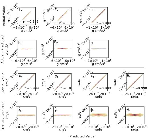
Fig 7. Error evaluation of a fully-connected network before any pruning. The seven
parameters shown are the outputs of the network, the three control variables and the
final derivatives of the state space. The residual plots are also shown (denoted by
Actual - Prediction).
January 7, 2022 18/22Fig 8. Error evaluation (with pruning) Note that axes for residual plots are
scaled to include the max outliers refref
January 7, 2022 19/22Table 2. Global parameters for the moth model. Below, we show a table of all
the required parameters to recreate the simulated model of a moth.
Label Value Units Description
L1 0.9 cm Length from the thorax-abdomen joint to the
center of mass of the head-thorax
L2 1.9 cm Length from the thorax-abdomen joint to the
center of mass of the abdomen
L3 0.75 cm Length from the thorax-abdomen joint to the
aerodynamic force vector
ρhead 0.9 g/cm2 The density of the insect head-thorax
ρbutt 0.4 g/cm2 The density of the insect abdomen
ρA 0.00118 g/cm3 The density of air
µA 0.000186 g/cm·s The dynamic viscosity of air at 27°C
ahead 0.9 cm Length of 1/2 major axis of head-thorax ellip-
soid
abutt 1.9 cm Length of 1/2 of major axis of abdomen ellipsoid
bhead 0.5 cm Length of 1/2 of minor axis of head-thorax
ellipsoid
bbutt 0.75 cm Length of 1/2 of minor axis of abdomen ellipsoid
K 23000 cm2 ·g/(rad·s2 ) Torsional spring constant of the thorax-
abdomen joint
c 14075.8 cm2 ·g/s Torsional damping constant of the thorax-
abdomen joint
g 14075.8 cm/s2 Acceleration due to gravity
βR 0 rad Resting configuration of the torsional spring =
(initial abdomen angle) - (initial head-thorax
angle) - π
t 0.02 s Time step
January 7, 2022 20/22Table 3. Calculated variables for moth model. Below, we show a table of all the
required calculated variables to recreate the simulated model of a moth.
Variable Expression Units Description
m1 ρhead · 34 π · (bhead )2 · ahead g Mass of head-thorax
m2 ρbutt · 34 π · (bbutt )2 · abutt g Mass of the abdomen
echead ahead /bhead N/A Eccentricity of head-thorax
ecbutt abutt /bbutt N/A Eccentricity of abdomen
1
I1 5 m1 · (bhead )2 · g·cm2 Moment of inertia of the head-
(1 + (echead )2 ) thorax
1
I2 5 m2 · (bbutt )2 · g·cm2 Moment of inertia of the abdomen
(1 + (ecbutt )2 )
Shead π · (bhead )2 cm2 Surface area of the head-thorax. In
this case, it is modeled as a sphere.
Sbutt π · (bbutt )2 cm2 Surface area of the abdomen.
In this case, it is modeled as
a sphere.
p
Rehead ρA · ẋ2 + ẏ 2 · N/A Reynolds number for the head-
(2 · bhead )/µA thorax
p
Rebutt ρA · ẋ2 + ẏ 2 · N/A Reynolds number for the abdomen
(2 · bbutt )/µA
Cdhead p |+
24/|Rehead N/A Coefficient of drag for the head-
6/(1 + |Rehead |) + 0.4 thorax
Cdbutt p |+
24/|Rebutt N/A Coefficient of drag for the abdomen
6/(1 + |Rebutt |) + 0.4
January 7, 2022 21/22Table 4. Initial state space and controls for generating training data. The
following variables are the required state space and control variables along with their
ranges for random uniform sampling.
Var. Distribution Units Variable type Description
x0 0 cm State Space Initial horizontal
position
ẋ0 U nif (−1500, 1500) cm/s State space Initial horizontal
velocity
y0 0 cm State space Initial vertical
position
ẏ0 U nif (−1500, 1500) cm/s State space Initial vertical ve-
locity
θ0 U nif (0, 2π) rad State space Initial head-
thorax angle
θ̇0 U nif (−25, 25) rad /s State space Initial head-
thorax angular
velocity
φ0 U nif (0, 2π) rad State Space Initial abdomen
angle
φ̇0 U nif (−25, 25) rad /s State space Initial abdomen
angular velocity
F U nif (0, 44300) g·cm/s2 Control Force magnitude
α U nif (0, 2π) rad Control Force angle
τ U nif (−100000, 100000) g·cm/s2 · cm Control Torque
Table 5. Final state space variables The following variables are the output from
the differential equation solver. These variables describe the final state space of the
insect after 20ms.
Variable Units Description
xf cm Initial horizontal position
ẋf cm/s Final horizontal velocity
yf cm Initial vertical position
ẏf cm/s Initial vertical velocity
θf rad Final head-thorax angle
θ̇f rad /s Final head-thorax angular velocity
φf rad Final abdomen angle
φ̇f rad /s Final abdomen angular velocity
January 7, 2022 22/22You can also read