Proton therapy of head and neck cancer: evaluation of PTV-based and robust optimized IMPT versus VMAT
←
→
Page content transcription
If your browser does not render page correctly, please read the page content below
Proton therapy of head and neck cancer:
evaluation of PTV-based and robust
optimized IMPT versus VMAT

Anja Einebærholm Aarberg

Master of Science in Physics and Mathematics
Submission date: June 2017
Supervisor:       Signe Danielsen, IFY
Co-supervisor:    Sigrun Saur Almberg, St. Olavs Hospital
                  Jomar Frengen, St. Olavs Hospital

Norwegian University of Science and Technology
Department of Physics
Abstract

Radiation therapy for head and neck cancers has had an essential role for curative treatment for
many years. Due to the location of the cancer, several critical organs will get irradiated and this
may lead to serious side-effects, such as xerostomia, dysphagia and secondary malignancies.
In this thesis the possible benefits of proton therapy is investigated by comparing Volumetric
modulated arc therapy (VMAT) and Intensity modulated proton therapy (IMPT) for patients
with oropharynx cancer. Two different techniques to achieve adequate target coverage were
tried out: planning target volume (PTV)-based IMPT and robust optimized IMPT.

The IMPT plans were kept equal (or better) in terms of target dose coverage as VMAT. The
mean parotid dose was then reduced as much as possible without losing target coverage. The
mean dose to both parotid glands were reduced for 8 of 12 patients with a corresponding reduc-
tion in the normal tissue complication probability (NTCP). It was shown that robust optimized
IMPT achieved the lowest mean parotid dose and also the lowest NTCP.

A repeat CT was taken halfway through the treatment and was used to check IMPTs robustness
for patient anatomy changes. The robust optimized IMPT was deemed the most robust, where
11 of 12 patients still had adequate target coverage. For medulla the maximum dose (50 Gy)
was exceeded for 1 patients for PTV-based IMPT and for none of the patients for robust opti-
mized IMPT. For 2 patients perturbed dose distributions were made and the robust optimized
IMPT plan was again deemed the most robust against set up uncertainties.

This study showed that some patients might benefit from IMPT, but for other patients VMAT
may yield the same treatment effects. Robust optimized IMPT should be preferred over PTV-
based IMPT.

                                                 i
ii
Samandrag

Stråleterapi for hovud- og halskreft har lenge hatt ei sentral rolle for kurativ behandling. Hovud-
og halsområdet har fleire kritiske organ som vil bli stråla samtidig som tumoren og dette kan
føre til seriøse biverknadar, som til dømes xerostomia, dysphagia og sekundær kreft. I denne
oppgåva er moglege fordelar av protonterapi sett på ved å samanlikne volumetrisk modulert
stråleterapi (VMAT) med intensitesmodulert protonterapi (IMPT) for pasientar med orophar-
ynx kreft. To ulike teknikkar for å få adekvat målvolumdekning er prøvd ut: PTV-basert IMPT
og robust optimisert IMPT.

Målvolumdekninga til IMPT-planane var uendra (eller betre) samanlikna med VMAT. Gjen-
nomsnittleg dose til parotis vart redusert så mykje som mogleg før det gjekk ut over målvolumdekninga.
Den gjennomsnittlege dosen til begge parotis blei redusert for 8 av 12 pasientar, med ein
tilsvarande redusering i normalvevskomplikasjonsraten (NTCP). Det blei vist at den robust op-
timaliserte IMPT-planen oppnådde dei lågaste gjennomsnittsdosane og NTCP-verdiar.

Ein ny CT blei tatt halvvegs i behandlinga og blei brukt til å sjekke robustheita til IMPT for
endringar i pasientanatomi. Robust optimaliserte IMPT blei ansett for å vere den mest robuste,
med målvolumdekning for 11 av 12 pasientar. For medulla var det 1 pasient som fekk over
50 Gy for PTV-basert og ingen for robust optimalisert IMPT. Perturberte doseplanar blei laga
for 2 pasientar og den robust optimaliserte IMPT-planen var igjen sett som den mest robuste.

Denne oppgåva viser at nokre pasientar vil ha fordel av behandling med IMPT, medan VMAT
gir same behandlingseffekt for andre pasientar. Robust optimalisering bør veljast over PTV-
baset IMPT.

                                                iii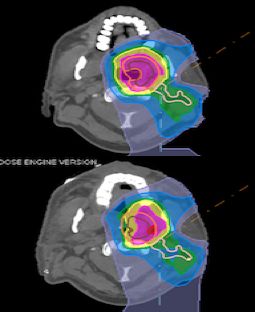
iv
Preface

This master thesis is written as the conclusion of my study of Biophysics and Medical Technol-
ogy at the Norwegian University of Science and Technology (NTNU). The work was done in
the spring of 2017 at the Department of Radiotherapy at St. Olavs Hospital.

I would like to thank my supervisor at St. Olavs Hospital, medical physicist Sigrun Saur Alm-
berg, for valuable help and guidance throughout the entire project work and writing process. I
would also like to thank co-supervisor Jomar Frengen for advice during the practical work of
this thesis. My supervisor at NTNU, Signe Danielsen, deserves a thanks, for the advice, feed-
back and encouragements given in the writing process of this master thesis.

A special thanks to Torbjørn Furre at Radiumhospitalet. And thank you, Liv Grønli Turtum, for
the encouragements throughout and proof-reading at the end.

Anja Einebærholm Aarberg
Trondheim, June 2017

                                              v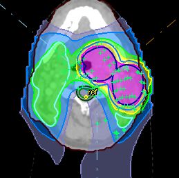
vi
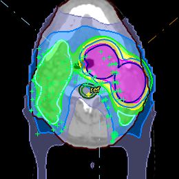
Table of Contents

Abstract                                                                                           i

Samandrag                                                                                         ii

Preface                                                                                           iv

Table of Contents                                                                                 vi

Acronyms                                                                                          x

1   Introduction                                                                                  1

2   Theory                                                                                        3
    2.1    Physics of radiation . . . . . . . . . . . . . . . . . . . . . . . . . . . . . . . .    3
           2.1.1   Absorbed dose . . . . . . . . . . . . . . . . . . . . . . . . . . . . . .       3
           2.1.2   Photon interactions . . . . . . . . . . . . . . . . . . . . . . . . . . . .     4
           2.1.3   Proton interactions . . . . . . . . . . . . . . . . . . . . . . . . . . . .     4
           2.1.4   LET and RBE . . . . . . . . . . . . . . . . . . . . . . . . . . . . . . .       7
    2.2    Generation of a clinical radiation beam . . . . . . . . . . . . . . . . . . . . . .     7
           2.2.1   Photon beam . . . . . . . . . . . . . . . . . . . . . . . . . . . . . . .       7
           2.2.2   Proton beam . . . . . . . . . . . . . . . . . . . . . . . . . . . . . . .       9
    2.3    Treatment planning . . . . . . . . . . . . . . . . . . . . . . . . . . . . . . . .     12
           2.3.1   CT . . . . . . . . . . . . . . . . . . . . . . . . . . . . . . . . . . . .     12
           2.3.2   Volume delineation . . . . . . . . . . . . . . . . . . . . . . . . . . . .     13
           2.3.3   Plan optimization . . . . . . . . . . . . . . . . . . . . . . . . . . . . .    15
    2.4    Plan evaluation . . . . . . . . . . . . . . . . . . . . . . . . . . . . . . . . . .    16
           2.4.1   Dose volume histogram . . . . . . . . . . . . . . . . . . . . . . . . .        16

                                                 vii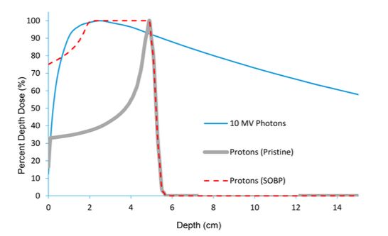
viii                                                                        TABLE OF CONTENTS

             2.4.2   NTCP modeling . . . . . . . . . . . . . . . . . . . . . . . . . . . . .        17
             2.4.3   Homogeneity index and conformity index . . . . . . . . . . . . . . . .         19
             2.4.4   Robust evaluation . . . . . . . . . . . . . . . . . . . . . . . . . . . . .    20

3      Method                                                                                       21
       3.1   Patients . . . . . . . . . . . . . . . . . . . . . . . . . . . . . . . . . . . . . .   21
       3.2   Treatment planning . . . . . . . . . . . . . . . . . . . . . . . . . . . . . . . .     22
             3.2.1   Volume delineation . . . . . . . . . . . . . . . . . . . . . . . . . . . .     22
             3.2.2   Plan optimization . . . . . . . . . . . . . . . . . . . . . . . . . . . . .    22
       3.3   NTCP . . . . . . . . . . . . . . . . . . . . . . . . . . . . . . . . . . . . . . .     25
       3.4   Plan evaluation . . . . . . . . . . . . . . . . . . . . . . . . . . . . . . . . . .    25
             3.4.1   Robust evaluation - perturbed treatment plans . . . . . . . . . . . . . .      26
             3.4.2   Statistical analyses . . . . . . . . . . . . . . . . . . . . . . . . . . . .   26
       3.5   Recalculating on new CT . . . . . . . . . . . . . . . . . . . . . . . . . . . . .      26

4      Results                                                                                      27
       4.1   Dose distribution - target volumes . . . . . . . . . . . . . . . . . . . . . . . .     27
             4.1.1   54Gy volume . . . . . . . . . . . . . . . . . . . . . . . . . . . . . . .      27
             4.1.2   60Gy volume . . . . . . . . . . . . . . . . . . . . . . . . . . . . . . .      28
             4.1.3   68Gy volume . . . . . . . . . . . . . . . . . . . . . . . . . . . . . . .      29
             4.1.4   Homogeneity Index . . . . . . . . . . . . . . . . . . . . . . . . . . . .      29
             4.1.5   Conformity Index . . . . . . . . . . . . . . . . . . . . . . . . . . . . .     31
       4.2   Organs at risk . . . . . . . . . . . . . . . . . . . . . . . . . . . . . . . . . . .   31
             4.2.1   Parotid glands . . . . . . . . . . . . . . . . . . . . . . . . . . . . . . .   31
             4.2.2   Medulla . . . . . . . . . . . . . . . . . . . . . . . . . . . . . . . . . .    32
             4.2.3   Irradiated volume . . . . . . . . . . . . . . . . . . . . . . . . . . . . .    33
       4.3   Re-CT . . . . . . . . . . . . . . . . . . . . . . . . . . . . . . . . . . . . . . .    34
             4.3.1   Target coverage - CTV . . . . . . . . . . . . . . . . . . . . . . . . . .      34
             4.3.2   Parotid Glands . . . . . . . . . . . . . . . . . . . . . . . . . . . . . .     36
             4.3.3   Medulla . . . . . . . . . . . . . . . . . . . . . . . . . . . . . . . . . .    37
       4.4   Perturbed treatment plans . . . . . . . . . . . . . . . . . . . . . . . . . . . . .    38

5      Discussion                                                                                   41
       5.1   Target volumes - VMAT vs IMPT . . . . . . . . . . . . . . . . . . . . . . . .          41
TABLE OF CONTENTS ix
5.2 Organs at risk - VMAT vs IMPT . . . . . . . . . . . . . . . . . . . . . . . . . 42
5.2.1 Parotid glands . . . . . . . . . . . . . . . . . . . . . . . . . . . . . . . 42
5.2.2 The use of NTCP . . . . . . . . . . . . . . . . . . . . . . . . . . . . . 43
5.2.3 Medulla . . . . . . . . . . . . . . . . . . . . . . . . . . . . . . . . . . 44
5.3 PTV-based IMPT vs robust optimized IMPT . . . . . . . . . . . . . . . . . . . 45
5.3.1 Re-CT . . . . . . . . . . . . . . . . . . . . . . . . . . . . . . . . . . . 45
5.3.2 Perturbed treatment plans . . . . . . . . . . . . . . . . . . . . . . . . 47
5.4 Field arrangement . . . . . . . . . . . . . . . . . . . . . . . . . . . . . . . . . 48
5.4.1 Spot placement . . . . . . . . . . . . . . . . . . . . . . . . . . . . . . 49
5.5 Dental fillings . . . . . . . . . . . . . . . . . . . . . . . . . . . . . . . . . . . 50
5.6 Future work . . . . . . . . . . . . . . . . . . . . . . . . . . . . . . . . . . . . 51
6 Conclusion 53
Bibliography 54
Appendices: 61
A Target dose coverage 63
B Organs at risk 69
C Perturbed treatment plans 71x TABLE OF CONTENTS
Acronyms

CT Computed tomography

CTV Clinical target volume

DVH Dose volume histogram

EUD Equivalent Uniform Dose

GTV Gross tumor volume

HU Hounsfield Unit

ICRU International Commission on Radiation Units and Measurements

IMPT Intensity Modulated Proton Therapy

IMPT-PTV Planning target volume-based IMPT

IMPT-Robust Robust optimized IMPT

IMRT Intensity Modulated Radiation Therapy

ITV Internal target volume

KVIST Kvalitetssikring i stråleterapi

LET Linear energy transfer

LINAC Linear Accelerator

LKB Lyman-Kutcher-Burman

NRPA Norwegian Radiation Protection Authority (Statens strålevern)

NTCP Normal tissue complication probability

                                            xi
xii TABLE OF CONTENTS OAR Organs at risk PTV Planning target volume RBE Relative biological effectiveness SFUD Single Field Uniform Dose SOBP Spread-out Bragg Peak TCP Tumor control probability VMAT Volumetric modulated arc therapy
Chapter 1

Introduction

Head and neck cancers include cancers of the mouth, lips, throat, nose, larynx and salivary
glands. In 2015 there were 774 new cases in Norway, corresponding to 2% of all new cancer
cases (1). The main portion of these are diagnosed with squamous cell carcinoma with the
primary tumor site often seen in the mucosa of the upper aeordigestive tract. The treatment of
choice (and prognosis) depend on the location and the probability of tumor spreading (2).

Head and neck cancers can be treated with surgery, chemotherapy and/or radiation therapy.
A combination of these are commonly needed for curative treatment and often also given for
palliative treatment. Techniques for photon radiation therapy used today are mainly Intensity
Modulated Radiation Therapy (IMRT), and a variant called Volumetric Modulated Arc Therapy
(VMAT) (3), which have resulted in better dose distribution and improved outcomes compared
to earlier radiation therapy techniques (4). Nevertheless, the treatment of head and neck cancer
is still associated with several side-effects because the target volumes are located close to several
organs at risk. Examples of side-effects are: xerostomia, dysphagia, neck fibrosis, esophageal
stenosis, hearing impairment, optic neuropathy, temporal lobe necrosis and secondary malig-
nancies (5).

Protons exhibit favorable properties for radiation therapy, they have finite range and the prospect
of delivering higher dose to the tumor without increasing the dose to the surrounding healthy
tissue. This may lead to sparing of normal tissues and organs at risk in the head and neck cases
(6). As a result of this several proton centers have begun giving proton therapy for head and
neck patients. One major problem that has presented itself is which patients benefit from pro-

                                                 1
2 CHAPTER 1. INTRODUCTION
ton therapy and this led to a group in the Netherlands introducing a model-based approach for
selecting patients who would likely benefit from Intensity Modulated Proton Therapy (IMPT)
based on normal tissue complication probability (NTCP) calculations (7).
A concern regarding IMPT, is that it is thought to be severely affected by uncertainties including
anatomical changes, patient setup errors and range uncertainties (8). There are two approaches
for taking setup errors and range uncertainties into account today; either add a geometrical mar-
gin to the target volume or apply robust optimization. The former is common for photons, but
is thought not to be adequate for proton therapy (9). Methods of robust optimization seek to
incorporate setup and range uncertainties in the treatment optimization by adding a number of
different possible scenarios to the optimization problem (10; 11). For head and neck cancer
patients, weight loss and shrinking of tumors during treatment are common, which can lead to
poor dose coverage of target volumes or increased dose to organs at risk. Adaptive radiotherapy
is suggested to account for this, and involves taking new CT scans for re-planning throughout
the course of the treatment (12).
In this master thesis the main focus has been to investigate the possible benefits of proton
therapy for head and neck cancers. The aims were:
1. Find suitable treatment parameters for IMPT of oropharynx cancer, including field num-
bers, angles and some standardized optimization criteria.
2. Investigate the potential in IMPT compared to VMAT for oropharynx cancer patients.
3. Investigate the robustness of the IMPT plans by recalculating the plans on CT scans taken
halfway through the treatment.
12 patients treated for oropharynx cancer at St. Olavs Hospital during 2016 were included in
the study.Chapter 2
Theory
The following chapter is in part based on and adapted from the authors project work in the
fall of 2016: ”Comparison of 3D-CRT, VMAT and Proton Therapy of Mediastinal Lymphoma”
(13).
2.1 Physics of radiation
Ionizing radiation is radiation that transfer sufficient energy to cause ionizations and excitations
in the medium it penetrates. The energy transfer is due to various atomic and nuclear interac-
tions, which will slow down and/or change the direction of the primary particle track. Photons
and neutrons are indirectly ionizing radiation because they release secondary particles in the
medium, which in turn causes ionizations. Charged particles are directly ionizing radiation
because they transfer the energy directly from the charged particle to the medium. (14)
2.1.1 Absorbed dose
To quantify the energy deposited in the medium the absorbed dose (D) is defined as the average
amount of energy imparted (dε) per unit mass (dm) of the irradiated medium (15):
dε
D= . (2.1)
dm
The absorbed dose is measured in Gy (J kg−1 ).
34 CHAPTER 2. THEORY
2.1.2 Photon interactions
A photon beam hitting a medium will be attenuated due to interactions. The attenuation of a
photon beam in matter is described by
I(x) = I0 e−µx , (2.2)
where I0 is the intensity of the photons before hitting the medium and I is the intensity of the
photons after passing a length, x, of the medium with a linear attenuation coefficient, µ (14). µ
is the probability of interaction per unit length and is dependent on the photon energy and the
atomic number of the medium.
Photons mainly interact with matter in three ways for therapeutic energies; photoelectric effect
(PE), Compton scattering (C) and pair production (PP). All of which result in the release of
secondary electrons that cause energy deposition in a medium. The total mass attenuation
coefficient is the probability of interaction (per unit length and mass) and is defined as
µ µPE µC µPP
= + + . (2.3)
ρ ρ ρ ρ
For external radiation therapy the energies range from 0.1 to 20 MeV and for these energies
the Compton scattering probability is dominating. Compton scattering depends on the electron
density of the medium, but is nearly independent of atomic number. The result of the interaction
is a photon with less energy than the primary photon and an electron. (14)
Interactions attenuate the photon beam, however not all photons will interact within the patient.
A portion of the photons will go straight through the patient without much energy loss. Photons
interact indirectly and this creates a build-up region, corresponding to the electron range, for
the dose as a function of depth. This is illustrated in figure 2.1 for the depth-dose curve of a
10 MV photon beam (in blue).
2.1.3 Proton interactions
Protons, here defined as heavy charged particles, interact with a medium in three different ways:
stopping, scattering and nuclear interactions.2.1. PHYSICS OF RADIATION 5
Figure 2.1: The depth-dose curve for photons (blue line), pristine protons (grey line) and spread-out
Bragg peak (SOBP) protons (red dotted line). It clearly shows a build up region and slow dose fall off
for the photons and the Bragg Peak, and rapid dose fall off for the protons. The illustration is borrowed
from (16).
Stopping
A charged particle will slow down in the medium by colliding with atomic electrons along its
path. The particle loses more energy the longer it interacts with the electrons, which means that
the amount of energy transferred depends on the velocity and charge of the particle, and density
of the medium. These energy losses can be described by the stopping power, defined as the
average energy loss, dE, per unit distance, dx, along the particle track in a medium (14).
The Bethe-Bloch formula gives a theoretical description of the stopping of heavy charged par-
ticles through matter:
dE ze2 2 4πZρNA h 2me v2 2 2
i
− = ln − ln(1 − β ) − β , (2.4)
dx 4πε0 Ame v2 I
where the different parameters and a description of these are found in table 2.1 (17). From
equation 2.4 it can be seen that the stopping power is inversely proportional to the velocity of
the particle squared, which explains the Bragg Peak for charged particles.6 CHAPTER 2. THEORY
Table 2.1: Parameters and description in the Bethe-Bloch formula for the stopping power of heavy
charged particles.
Parameter Description
ze Charge of the incident particle
me Electron mass = 0.511 MeV/c2
Na Avogadro’s number = 6.022 · 1023 mol−1
I Mean energy required to ionize an atom in the medium
Z, A Atomic number and atomic weight of the absorber medium
ρ Material density
β v/c of incident particle
For a proton beam it will be a prominent peak (the Bragg Peak) at a depth, depending on the
protons energy. This is because the proton deposits more dose as it slows down and as it nearly
stops it deposits the rest of the energy within a small area, as seen in figure 2.1 (in grey). This
figure also shows a spread-out Bragg Peak (SOBP) in red, which is created by summing the
depth doses from protons of different initial energy. A SOBP is used clinically to cover the
target volume.
Scattering
A proton incident on a medium will also collide with atomic nuclei, and because both the proton
and the nuclei are positively charged, the proton (much smaller mass than the nucleus) will
deflect from its path. The scattering angle from one such collision is very small and therefore
negligible, but after several collisions the scattering might be considerable. The summation of
all of these small deflections is a statistical observation and is often called multiple Coulomb
scattering (18).
Nuclear interaction
In addition to stopping and scattering, the proton may collide head-on with the atomic nucleus
in the medium. This effect is not prominent but has to be considered when dealing with proton
beams. When the proton collides with the nucleus, fragments of the nucleus will be set in
motion. These fragments may be protons, neutrons, electrons or larger fractions of the nucleus.
The fragments tend to have lower energies and deposits dose just downstream of the reaction
site before they stop. (18)2.2. GENERATION OF A CLINICAL RADIATION BEAM 7
2.1.4 LET and RBE
Linear energy transfer (LET) is defined as the average energy locally imparted to the medium by
a charged particle of specified energy in traversing a distance in that medium (15). LET has the
unit keV µm−1 and describes the density of ionization’s along the particles path. High-LET radi-
ation are densely ionizing radiation such as energetic neutrons, proton and other heavy charged
particles. Low-LET radiation are sparsely ionizing radiation, such as photons. The high-LET
radiation will produce more cell killing per Gy, but for very high-LET (LET > 100 keV µm−1 )
radiation the cell killing is less efficient. This is due to overkill, which means that the radia-
tion waste energy on cells that are already dead and therefore there is less likelihood per Gy
that other cells in the tissue will be killed (19). For protons the LET will increase as the energy
deposited to the medium increases, i.e. the LET increases as the beam pass through the medium.
For different radiation qualities the effect of the absorbed dose is not necessarily the same:
biological effects must also be taken into account. The relative biological effectiveness (RBE)
is defined as:
dose of reference radiation
RBE = , (2.5)
dose of test radiation
where the test refers to the radiation quality that is to be compared to the reference radiation
quality (19). The reference beam is usually low-LET 250 kVp X-rays (19), but Cobolt-60 rays
(1.25 MeV) are also used (20). The RBE vary with radiation quality, but also with fractionation,
cell type and dose rate. Protons are slightly more biologically damaging than photons and the
RBE mostly depends on LET. The RBE of the protons depend slightly on depth and will be
highest at the Bragg peak (21). Even so, a constant RBE of 1.1 is usually set for protons used
clinically (22). The value of 1.1 is based on experiments done in the 1950’s and seems to be a
reasonable constant value for clinical beam energies (21).
2.2 Generation of a clinical radiation beam
2.2.1 Photon beam
The most commonly used radiation quality in therapy today is photons, created by a linear
accelerator (linac). In a linac, electrons gain energy by interacting with a synchronous radio-8 CHAPTER 2. THEORY frequent electromagnetic field before bending and hitting a target (14). The interaction between electrons and the target releases photons (bremsstrahlung). A schematic drawing of a linac can be seen in figure 2.2. The photon beam can be shaped by collimators to hit an area of choice, such as a tumor. Figure 2.2: A schematic drawing of a linear accelerator used for photon based radiation therapy. The electrons interact with a electromagnetic field in the accelerating waveguide before hitting a target and producing photons (14). The introduction of modern techniques for treatment planning and delivery, i.e. IMRT, of head and neck cancer has decreased the toxicities associated with radiation therapy, and also in many cases increased the local control of the cancer (3). IMRT is a technique that produces conform dose distributions by varying the intensity of the radiation beam during treatment, illustrated in figure 2.3a. Also seen in figure 2.3b is an example dose distribution of a head and neck treat- ment plan using IMRT. IMRT is applied to complex target volumes to conform the distribution to the target volume and limit the dose to nearby organs at risk. In IMRT, multiple non-uniform radiation fields are used and shaped according to the projection of the target volume, taking into consideration dose- volume objectives of the surrounding volumes. IMRT is an iterative technique which utilizes inverse planning; the user defines constraints and objectives, which the iteration algorithm will take into consideration to solve the treatment planning problem. (23) VMAT Volumetric modulated arc therapy (VMAT) is a variant of the IMRT-technique were the gantry moves continuously around the patients while the dose rate and field shape vary with the posi- tion of the gantry (24). The treatment can be delivered in one or more arcs, depending on the location and complexity of the tumor. Typically, a checkpoint every ∼ 4◦ ensures proper dose
2.2. GENERATION OF A CLINICAL RADIATION BEAM                                                        9

                         (a)                                               (b)
Figure 2.3: IMRT, (a) schematic drawing of intensity modulation (23) and (b) an example dose distribu-
tion (24) for a head and neck case.

delivery. The main advantage of VMAT over IMRT is the speed of treatment delivery; typically
2-3 minutes for VMAT versus 10-20 minutes for IMRT. (20)

2.2.2    Proton beam

To accelerate protons to clinical beam energies to reach the desired depths either a cyclotron or
a synchrotron is used. As the cyclotron is the most common among clinical installations it will
be briefly described here.

Cyclotrons accelerate protons to a fixed energy that are modulated with a degrader to deliver the
intended energies to the patient. It is a short metallic cylinder consisting of two metal electrodes,
called dees, where a varying electric potential will accelerate the incoming charged particle. A
magnetic field is set up perpendicular to the electric field so that the particle spirals out towards
the edge of the dees when its energy is increased (20). Combining the Lorentz force, FB = qvB,
                                                                 mv2
and the centripetal force for non-relativistic particles, FC =    r ,   gives

                                                  mv2
                                            qvB =
                                                   r

                                                    qBr
                                              v=        .
                                                     m
                                          mv2
The kinetic energy of the particle, E =    2 ,   can thus be written as
10 CHAPTER 2. THEORY
(qBr)2
E= . (2.6)
2m
The maximum particle energy depends on the radius of the electrodes of the cyclotron and the
strength of the magnetic field, B. The maximum energy for a cyclotron is about 250 MeV and
when the particle reach this energy it is ejected and transported towards the treatment room (20).
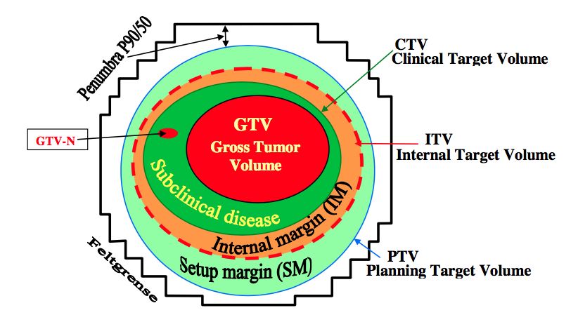
Figure 2.4: Example of possible setup for (top) passive scattering and (bottom) active scanning (25).
There are two methods of delivering proton therapy: passive scattering and active scanning (26).
Passive scattering use materials with high atomic numbers to scatter the beam to usable lateral
dimensions and then modulate the energy creating a so called spread out Bragg Peak (SOBP)
to cover the desired depth, as seen in figure 2.4 (top). Active scanning or beam scanning is a
technique that deflects the beam across the target by moving the pencil beam, as illustrated in
figure 2.4 (bottom). The beam is usually steered by magnets that deflect the beam so that the
whole target can be covered. Active scanning is used for a technique called single field uniform
dose (SFUD) where individually optimized pencil beams from each field delivers a homoge-
neous dose to the target volume. The goal is to deliver a dose distribution across the target that
is as homogeneous as possible (26).
Active scanning can deliver intensity modulated proton therapy (IMPT), analogous to IMRT
for photons, by varying the fluence in each spot of the scan and/or the beam intensity. The
dose can be delivered non-uniformly on a field-by-field basis, and add up to a uniform target2.2. GENERATION OF A CLINICAL RADIATION BEAM 11 dose. IMPT simultaneously optimizes the pencil beams from all the fields. Each field may not be homogeneous across the target but the dose distribution from all fields will still be homo- geneous. IMPT place the Bragg peaks throughout the target volume and give them adjusted weights across the target, as homogeneously as possible (26). Although passive scattering has been used the longest, the use of active scanning techniques are increasing, and are considered to be the future of proton therapy. Proton planning for head and neck cancer today IMPT is currently being used in several proton centers around the world to treat head and neck cancer. Two well-recognized centers are MD Anderson and the Paul Sheffer Institute (PSI). They use different field arrangements clinically, and below is a brief summary of both. MD Anderson use a three field configuration; two anterior oblique beams (±50◦ − 70◦ ) and one posterior beam (180◦ ), illustrated in figure 2.5a. They also use a couch angle for the anterior beams of 15◦ − 20◦ . This is done to optimize the target coverage and minimize the dose to unnecessary tissue and organs at risk (OAR). Another reason for this choice is to reduce uncer- tainties in proton range by avoiding irradiating through the mouth. (27) Figure 2.5: a) Snapshot showing MD Anderssons field configuration and b) figure from (28) showing the field configuration used at PSI. PSI use a 4 field star-technique, as seen in figure 2.5b, using two anterior, oblique (±60◦ ) beams and two posterior oblique (±100◦ ) beams to deliver the prescribed dose. The reason for this is to provide robust coverage of the target volumes. (28; 29)
12 CHAPTER 2. THEORY
2.3 Treatment planning
2.3.1 CT
To begin treatment planning the anatomy of the patient is imaged by a CT scan. The unit used
in CT is Hounsfield unit (HU) and is defined as:
µ − µwater
HU = 1000 · , (2.7)
µwater
where µ is the linear attenuation coefficient, and HU = -1000 for air and HU = 0 for water. It is
common to use a mass density of 0.001 21 g/cm3 for all HU values less than -1000 and a mass
density of 7.87 g/cm3 for HU above 2800 (30).
For treatment planning the HU numbers are converted into electron mass densities that can be
used to identify the different tissues in the patient. A snapshot from RayStation (RaySearch
Laboratories) illustrates this relationship in figure 2.6. For proton therapy the HU numbers are
converted into proton stopping power values using a calibration curve (18). Errors in the HU
numbers will therefore translate into uncertainties in the range of protons. A CT with high pre-
cision is needed for proton therapy in order to minimize the range uncertainties.
Figure 2.6: CT Hounsfield units to density conversion graph, taken from RayStation interface (30).
As any imaging modality, CT is prone to artifacts. An example of metal artifacts is shown in
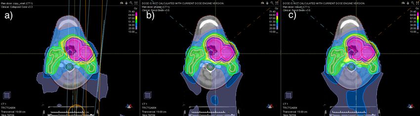
figure 2.7. CT image reconstruction is performed using a filtered back projection method, which2.3. TREATMENT PLANNING 13 Figure 2.7: Example CT scan from a patient with titanium implants in the cervical spine and dental fillings, image from Verburg and Seco (31). assumes monochromatic x-ray attenuation and a complete set of projection measurements (31), and can result in artifacts. The metal artifacts can have great impact on the dose calculation and should be taken into account when making treatment plans. 2.3.2 Volume delineation Volume structures are delineated on the CT images by a physician before any treatment planning can be done. A region of interest (ROI) is usually either a target or an organ at risk (OAR). The following description of the ROIs are based on the KVIST-group report form the Norwegian Radiation Protection Authority (NRPA) (32), which again is based on ICRU report 83 (33). Target volumes The target volumes are divided into several areas with different margins to account for uncer- tainties, as can be seen in figure 2.8. The gross tumor volume (GTV) is the solid or demonstrable tumor one can identify from the images taken. The clinical target volume (CTV) is the GTV with margins that account for sub-clinical spread in the tissue and involvement of elective areas. This is the volume that should be treated. The internal target volume (ITV), takes the uncertain- ties in position of the CTV in the patient into account. Around the CTV (or ITV), a planning target volume (PTV) is delineated to take into account patient motion and uncertainties in setup and delivery of the treatment. The PTV is used to ensure that the prescribed dose actually is delivered to the CTV.
14                                                                        CHAPTER 2. THEORY

       Figure 2.8: Illustration of target volumes and margins defined by the KVIST-group (32).

Risk volumes

Organs at risk (OAR) are delineated to ensure that radiation sensitive tissue, that may limit
the treatment plan, are taken into account. A planning organ at risk volume (PRV) are often
added for serial organs in the same way as a PTV is added to the CTV to take into account
uncertainties. All tissues could be regarded as OAR as irradiating healthy tissue is known to
enhance the risk for late radiation effect, but usually only organs with critical function close to
the CTV are delineated.

Patient uncertainties in proton therapy

IMPT is thought to be heavily affected by uncertainties because of the precision in which the
beam is delivered and the conformity of the dose distribution (steep gradients of the pencil
beams). The most prominent uncertainties are anatomical changes, patient setup errors and
range uncertainties. The anatomical changes can be organ motion, changes in the sinuses (air
cavities), tumor volume increase/decrease and/or patient weight loss or gain. The range un-
certainties come from uncertainties regarding the Hounsfield units (HU) used for the images
taken with computed tomography (CT) and the conversion between HUs into stopping power
for protons. (8)
2.3. TREATMENT PLANNING 15
To account for uncertainties in photon radiation therapy a planning target volume (PTV) is usu-
ally made from the clinical target volume (CTV). The margin between the PTV and the CTV is
determined based on setup errors and tumor movement, since range uncertainties in photons are
of far less importance than for protons. In the literature today several articles do not recommend
the use of a PTV for protons (9; 11; 34; 35) and they suggest instead the use of a robust opti-
mization method to account for both setup error and range uncertainties. Methods have been
proposed in several articles (11; 34; 36) and the robust method is now regarded by many as the
best way to make the proton treatment plans robust against uncertainties.
2.3.3 Plan optimization
Inverse planning
Inverse planning is an optimization technique where the user defines different criteria for a
treatment plan, and lets the optimizer find the best solution to the problem. The objective
function can be defined as:
S
F(x) = ∑ λσ(Dσ − d σ)2 (2.8)
σ=1
Dσ = Aσ x σ = 1, ...., S; x ≥ 0,
where σ defines the structure (i.e., an OAR or a target volume), λσ is a structure-specific weight-
ing factor, Dσ is the calculated dose and d σ is the prescribed dose, Aσ is the dose kernel matrix
and x is the intensity of the beam (37). The goal of inverse planning is to minimize the objective
function, e.g. find the global minimum.
A robust optimization method
One way of implementing robust optimization is to use a minimax optimization, where the
optimization functions are selected to minimize the objective function in the worst case scenario
(11). This gives a threshold for how much the treatment plan quality can deviate due to errors.
The worst case scenario is a realization of uncertainty under which a robust function attains its
highest value. For several functions, n, the minimax optimization can be formulated as16 CHAPTER 2. THEORY
n
min max ∑ wi fi (d(x; s)), (2.9)
x∈X s∈S
i=1
where X is the set of feasible variables and S is the scenarios included in the optimization. d(x; s)
is the dose distribution as a function of the variables x and the scenario s (11). With this method
the information about the uncertainties and errors are incorporated into the optimization and it
enables the treatment planning system to determine where to deposit dose to achieve plans that
are robust against setup error and range uncertainties.
Practical plan optimization
In a treatment planning system the above is implemented and the user defines objectives for
the target volumes and organs at risk. Examples of objectives are minimum dose to the target
volumes, mean dose to a volume and/or maximum dose to an organ at risk. When the objectives
are decided the weighting can be modified so that the most important, often target coverage, has
the highest weight and thus has precedence over other volumes. The plan can then be iterated
until the user is satisfied with the dose distribution and the treatment plan can be administered
to the patient.
2.4 Plan evaluation
2.4.1 Dose volume histogram
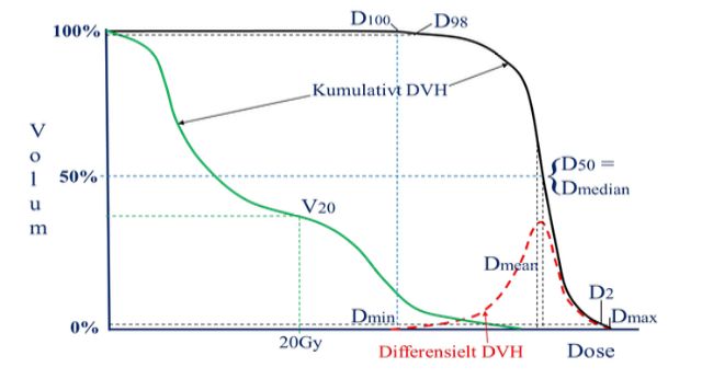
A dose volume histogram (DVH) is a representation of radiation dose as a function of volume.
A cumulative DVH show the volume elements receiving at least a given dose value (33). Illus-
trated in figure 2.9 and relevant to the plan evaluation process is the different DV parameters
that describe the minimum dose to a volume, V. Another parameter is VD , which is the volume
receiving a dose greater or equal than D. A parameter often used for the minimum dose value in
a dose distribution is D98 , this is the dose at least 98% of the volume receives. For the maximum
dose value D2 is often reported, that is the dose that maximum 2% of the volume receives.2.4. PLAN EVALUATION 17 Figure 2.9: Example of DVH and parameters associated with treatment plan evaluation (32). Black: target volumes and green: organs at risk. 2.4.2 NTCP modeling To visualize the goal of radiation therapy; to deliver enough dose to the tumor and as low dose as possible to the surrounding tissue, a helpful parameter is the therapeutic ratio. The therapeutic ratio is defined as the ratio between the tumor control probability (TCP) and the normal tissue complication probability (NTCP) at a given level of response. It can be illustrated as in figure 2.10, where curve A is the TCP and curve B is the NTCP. The goal is to have the NTCP curve as far to the right of the TCP curve as possible and thus achieve the greatest therapeutic ratio. The therapeutic ratio depends on fractionation, treatment time and technique, target volume, LET and dose rate (38). LKB model NTCP models are a tool for treatment plan evaluation, where the main idea is to estimate the probability for normal tissue complications from the DVH given by the treatment planning sys- tem. A frequently used NTCP-model is the Lyman-Kutcher-Burman (LKB) model (39; 40). To report non-uniform dose distribution the equivalent uniform dose (EUD) was introduced in 1997 by Niemierko (41). The EUD assumes that two dose distributions are equivalent if the radiobiological effect is the same and is given by
18                                                                           CHAPTER 2. THEORY

Figure 2.10: Illustration of curves for A: tumor control probability (TCP) and B: normal tissue complica-
tion probability (NTCP). The therapeutic ratio can be found by the ratio of TCP and NTCP at a specified
dose (38).

                                        EUD = ∑(Di a vi )1/a ,                                    (2.10)
                                                  i

where Di is the dose to voxel i and vi is the relative volume of the voxel. a is a tissue-specific
parameter that is determined by comparing tumor and normal tissue response. For serial organs
a has a large value while for parallel organs it is closer to 1 (42).

The LKB model is an empirical NTCP model and use a cumulative Gauss function to charac-
terize the NTCP. Mohan et. al (43) proposed a mathematical representation of the NTCP curve,
which begins with an integral of the normal distribution

                                                      Z t
                                             1                   2 /2
                                     NTCP = √               ex          dx                        (2.11)
                                             2π        −∞

where

                                                 D − T D50
                                            t=             ,                                      (2.12)
                                                  mT D50

m describes the steepness of the NTCP-curve and T D50 is the dose corresponding to a NTCP
of 50%. D is given by
2.4. PLAN EVALUATION 19
D = ∑(Di 1/n vi )n (2.13)
i
and is thus equal to the EUD when n = 1/a. The parameters needed for calculating NTCP using
the LKB model is T D50 , n and m. The parameters are empirically derived by fitting the NTCP
predictions for an endpoint to data from clinical outcomes for a population of treated patients
(44).
2.4.3 Homogeneity index and conformity index
The homogeneity index (HI) characterizes the homogeneity of the dose within the target volume
(33). In RayStation (30) it is defined as:
D(x)
HI = , (2.14)
D(100-x)
where D(x) is the dose at x% of the volume. A homogeneity index of 1 indicates a completely
homogeneous dose distribution over the entire target volume.
The conformity index (CI) gives an indication of how conform the dose to the target volume is
and is in RayStation (30) defined as:
Vtarget volume
CI = , (2.15)
Vtreated volume
where Vtarget volume is the volume of the delineated target volume (often the PTV) and Vtreated volume
is the volume covered by a total isodose volume, where the 90% or 95% isodose is the most
common to use. A conformity index near 1 indicates good conformity. A shortcoming of the
CI is that it does not take into account the degree of spatial intersection of the volumes or their
shapes (45). The CI can therefore be 1 without the volumes being similar or in the same area.
It is therefore important to use this index in addition to visualization tools for the dose distribu-
tion, so that the risk of a total miss is minimized.20 CHAPTER 2. THEORY 2.4.4 Robust evaluation A method to evaluate the robustness of a treatment plan is to do a geometric shift of the isocen- ter, recalculate the plan and evaluate the resulting dose distribution. In a similar manner, the CT densities can be changed and the effect evaluated after re-calculation.
Chapter 3

Method

3.1     Patients

The patients in this master thesis were included in a previous project at St. Olavs Hospital.
The project investigated the need for re-planning of VMAT plans for head and neck cancers
based on an extra CT exam taken after 18 fractions. To be included in the original project pa-
tients had to get curative radiation treatment for head and neck cancer at St. Olavs Hospital,
and lymph nodes had to be included in the radiation field, receive at least a dose of 60 Gy and
have adequately cognitive function. The patients provided informed consent and the study was
approved by REK (2015/2022). A subgroup of patients with oropharynx cancer from the study
was selected for this master thesis.

In total 12 patients with oropharynx cancer were included in the present study. Patient infor-
mation is given in table 3.1. The mean age was 61.3 years old (range: 55-79) and the staging
of the cancer ranged from T2 to T4, local nodal involvement was common and none of the
patients had metastases. The repeat CT was normally taken at the 18. treatment fraction, that
is after 36 Gy. All plans, VMAT, PTV-based IMPT (IMPT-PTV) and robust optimized IMPT
(IMPT-Robust), were made in RayStation v.5.0. The treatment machine used for VMAT was
Agility Thr feb and for IMPT the machine RSL IBA UNI was used.

                                              21
22 CHAPTER 3. METHOD
Table 3.1: Information about the patients included in the present study.
Study # Gender Age Primary tumor TNM stage Dental fillings
1 Male 63 Tonsil T2N0M0 No
2 Female 61 Tonsil T4aN2bM0 Yes
3 Male 59 Base of tongue T1N2aM0 Yes
4 Male 55 Tonsil T4aN2cM0 Yes
6 Male 79 Tonsil T4aN2bM0 Yes
9 Female 62 Tonsil T1N2aM0 No
13 Female 57 Base of tongue T4aN0M0 Yes
18 Male 60 Tonsil T2N2bM0 Yes
19 Male 67 Tonsil T2N2bM0 Yes
20 Male 55 Tonsil T2N2bM0 Yes
21 Male 56 Tonsil T2N2bM0 No
23 Male 62 Tonsil T2N2bM0 Yes
3.2 Treatment planning
The clinical target volumes were divided into three: a high risk volume to receive 68 Gy
(CTV68), a intermediate risk volume to receive 60 Gy (CTV60) and low risk volume to receive
54 Gy (CTV54). The clinical target volume therefore included the primary disease, involved
lymph nodes and potential areas of subclinical spread. For VMAT and PTV-based IMPT the
CTVs were expanded with 5 mm to create corresponding PTVs. CTV54ex /PTV54ex are the
CTV54/PTV54 volumes without CTV60/PTV60 and CTV68/PTV68.
3.2.1 Volume delineation
Target volumes and organs at risk were delineated by a physician on the treatment planning
CTs, a representative delineation of the CTVs and PTVs is shown in figure 3.1. In addition,
volumes specific to IMPT-planning were made. The CTVs, parotid glands and medulla were
transferred from the original CT to the re-CT using deformable registration. The volumes were
evaluated and adjusted (if needed) by the responsible physician.
3.2.2 Plan optimization
Two IMPT plans were made for each patient, one based on PTV (IMPT-PTV) and one with ro-
bust optimization (IMPT-Robust). Based on literature it was decided to use two oblique anterior
beams (50◦ and 310◦ ) and one posterior beam (180◦ ), see figure 3.2, similar to what is used at
MD Andersson (27).3.2. TREATMENT PLANNING 23
(a) (b)
Figure 3.1: Target volume delineation for patient 21 of (a) CTVs and (b) PTVs. Pale pink: CTV54ex ,
Magenta: CTV60, Pink: CTV68, Bright blue: PTV54ex , Blue: PTV60, Dark blue: PTV68.
310◦ 50◦
180◦
Figure 3.2: Field angles for IMPT for head and neck cancer.24 CHAPTER 3. METHOD
The optimization objectives are shown in table 3.2. The minimum dose objectives for the differ-
ent CTVs were given the highest weight because the CTV coverage has precedence over the rest
of the objectives. The initial parotid dose objective was determined from the original VMAT
plan, and then reduced as much as possible without compromising the target coverage.
Table 3.2: Optimization objectives used for IMPT.
ROI Objective Robust-function
CTV68 Uniform dose Yes
CTV68 Minimum dose Yes
CTV60 Minimum dose Yes
CTV54ex Minimum dose Yes
CTV54ex Uniform dose Yes
Parotid Max EUD No
Medulla Max dose Yes
External Dose fall-off No
For patients 1-13 a range shifter of 40 mm was applied to all of the beams. For patients 18-23
a range shifter of 75 mm was applied to the two anterior beams and 40 mm for the posterior
beam. Furthermore for patients 18-23 the anterior beams were restricted to treat the same side
as the elective node only, this was done with objectives with zero weight applied to the left or
right side of PTV54. Patient 1 was a unilateral case and for that patient the contralateral beam
was removed to avoid unnecessary irradiation of healthy tissue.
The objectives chosen for the IMPT-Robust plans are given in table 3.2, in addition to which
objectives were optimized with the robust-function. The robustness settings were set to 5 mm
spatial shift in 6 directions and ±3% density change.
To evaluate the plans in a fast and easy manner, clinical goals were specified and utilized as a
first impression on the quality of the treatment plan. Isodoses, DVHs and dose statistics were
studied for further evaluation of the plans. If the plan was not deemed adequate modification
of the objectives and further iterations had to be done. To be acceptable the IMPT plans were
required to have a comparable target dose coverage as VMAT and the comparison was then
done based on dose characteristics to the organs at risk.3.3. NTCP 25
3.3 NTCP
It was of interest to evaluate not only the dose change to the parotid glands between VMAT and
IMPT but also if the probability of normal tissue complication was decreased for IMPT.
Figure 3.3: Picture from CERR showing the window for NTCP modeling.
NTCP values for parotid glands were calculated using the MATLAB (The Mathworks, Inc.)
based program CERR (Computational Environment for Radiotherapy Research) (46). CERR
calculates NTCP values from imported DVHs. A choice of NTCP models is offered as well
as the possibility to change the parameters of the model. A snapshot of the window for NTCP
modeling is shown in figure 3.3. In this thesis the LKB model was chosen with parameters n =
1, m = 0.4 and TD50 = 39.9, based on values for the parotid gland presented by Houweling et
al. (47). To define a complication the threshold in this study was set to 25% of original saliva
flow one year after the radiation treatment.
3.4 Plan evaluation
The main focus was the dose coverage to CTV, the mean dose to parotid glands and the max-
imum dose to medulla. D98 was chosen for evaluation of the target coverage, D2 was also26 CHAPTER 3. METHOD extracted for the target volumes for comparison with VMAT. For VMAT and IMPT-PTV, V95 and V105 was also evaluated. The homogeneity index, equation 2.14, was calculated using x = 95%, while the conformity index, equation 2.15, was calculated using the 90% isodose. 3.4.1 Robust evaluation - perturbed treatment plans Robust evaluation was done for 2 patients. The isocenter was shifted by 5 mm in 6 directions and the treatment plan was recalculated. Dose statistics on the CTVs and parotid glands were extracted. 3.4.2 Statistical analyses To test for statistical significance a Student’s t-test was used. The MATLAB function ttest(x,y) uses the paired-sample t-test and returns a test decision for the null hypothesis that the data in x and y comes from a normal distribution with mean equal to zero and unknown variance. The default setting is a 0.05 significance level (48). The t-test was used for both mean dose and NTCP of parotid glands, maximum dose to medulla and target volume coverage - checking for statistical significance in the difference between VMAT and IMPT and also between the origi- nal CT and re-CT for IMPT plans. Box plots were made using MATLAB, where the red line are the median value (q2 ). The edges of the box is the 25th percentile (q1 ) and the 75th percentile (q3 ). The outliers are shown in red plus-signs and a data point is defined as an outlier if it is larger than q3 + w(q3 − q1 ) or smaller than q3 − w(q3 − q1 ). w is the maximum whisker length and is set by default to 1.5. (48) The black crosses are the mean values. 3.5 Recalculating on new CT In the original project a new CT was taken after 18 fractions and recalculated treatment plans were made for VMAT. In the present study the second CT was used to recalculate the origi- nal IMPT treatment plans to see if the plans are robust against uncertainties related to patient anatomy. Relevant dose statistics (CTV coverage and mean dose to parotid glands) were ex- tracted and compared to the original CT for both IMPT-PTV and IMPT-Robust.
Chapter 4
Results
4.1 Dose distribution - target volumes
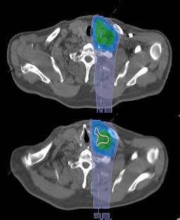
In figure 4.1 a snapshot from RayStation showing the dose distribution for a representative pa-
tient of this project work. The volumes of interest for target coverage is CTV54ex , CTV60 and
CTV68 for all plans, and PTVex , PTV60 and PTV68 for VMAT and IMPT-PTV. From figure
4.1 it is seen that all treatment techniques give conformal dose distributions and cover the target
volumes. Also seen is the low-dose bath that is associated with VMAT, which is one of the
reasons for investigating IMPT for therapy.
Figure 4.1: Example of dose distribution (patient 21) for a) VMAT b) IMPT-PTV c) IMPT-Robust taken
from a representative patient. Pink: 64.6 Gy, Yellow: 57 Gy, Green: 51.3 Gy, Blue: 34 Gy.
4.1.1 54Gy volume
Dose distribution parameters for CTV54ex are shown in box plots in figure 4.2b and 4.2a. Mean
D98 to CTV54ex was 53.1 Gy for VMAT, 52.8 Gy (p = 0.006) for IMPT-PTV and 52.5 Gy
2728 CHAPTER 4. RESULTS
62 66
CTV54 ex CTV54 ex
60 64
58 62
D98 [Gy]
D2 [Gy]
56 60
54 58
52 56
50 54
VMAT IMPT-PTV IMPT-Robust VMAT IMPT-PTV IMPT-Robust
(a) (b)
100 10
PTV54 ex PTV54 ex
98 8
V105 [%]
96 6
V95 [%]
94 4
92 2
90 0
VMAT IMPT-PTV VMAT IMPT-PTV
(c) (d)
Figure 4.2: Dose/volume parameters of CTV54ex /PTV54ex for all patients. (a) Dose given to at least 98%
of CTV54ex [D98 ]. (b) Dose given to the hottest 2% volume of CTV54ex [D2 ]. (c) Volume receiving 95%
of 54 Gy. [V95 ]. (d) Volume receiving 105% of 54 Gy [V105 ]. The dotted line indicates for (a) 95% and
(b) 105% of 54 Gy.
(p = 0.002) for IMPT-Robust. The p-values are calculated with a paired-sample t-test as de-
scribed in section 3.4.2. For all patients, D98 to CTV54ex was > 95% dose level (51.3 Gy),
which is required for the target volume. D2 was for all patients > 105% dose level (56.7 Gy)
for VMAT, whereas for IMPT 9 and 4 patients were > 105% dose level for IMPT-PTV and
IMPT-Robust, respectively.
In figure 4.2c the volume of PTV54ex receiving at least 95% of the prescribed dose is shown.
The mean values of V95 for PTV54ex is 97.9% for VMAT and 98.6% (p = 0.05) for IMPT-PTV.
For V105 (56.7 Gy), as shown in figure 4.2d, the mean value was 1.7% for VMAT, 0.99% for
IMPT-PTV and 0.94% for IMPT-Robust. The largest volume receiving 105% of the prescribed
dose for PTV54ex was 7% for VMAT and 5% for IMPT-PTV. Patient specific dose/volume
parameters are given in appendix A.
4.1.2 60Gy volume
The dose distribution parameter, D98 , for CTV60 is shown in figure 4.3a. All patients plans
were > 95% dose level. In figure 4.3b the volume of PTV60 receiving at least 95% of 60 Gy4.1. DOSE DISTRIBUTION - TARGET VOLUMES 29
68 100
CTV60 PTV60
66 98
64 96
D98 [Gy]
V95 [%]
62 94
60 92
58 90
56 88
VMAT IMPT-PTV IMPT-Robust VMAT IMPT-PTV
(a) IMPT-PTV (b) IMPT-Robust
Figure 4.3: Dose/volume parameters of CTV60/PTV60 for all patients. (a) Dose given to at least 98% of
CTV60 [D98 ]. (b) Volume receiving 95% [V95 ] of 60 Gy. The dotted line indicates 95% of 60 Gy.
is given. The mean values of V95 for PTV60 was 98.5% for VMAT and 99.26% (p = 0.04) for
IMPT-PTV. More detailed data is given in appendix A.
4.1.3 68Gy volume
For CTV68 the mean values of D98 are 67.1 Gy, 66.9 Gy (p < 0.01) and 66.1 Gy (p = 0.3) for
VMAT, IMPT-PTV and IMPT-Robust, respectively. The distribution for D98 is seen in figure
4.4a. Figure 4.4b shows the maximum dose, D2 , for CTV68 and all patient plans were below
the recommended 105% of 68 Gy, as seen by the dotted line.
The volume receiving 95% of the prescribed dose is shown in figure 4.4c. The mean values of
V95 for PTV68 was 98.1% for VMAT and 99.4% (p = 0.02) for IMPT-PTV. V105 , shown in
figure 4.4d, was small for both VMAT and IMPT-PTV, the largest volume receiving 105% of
68 Gy was 0.7%. Patient specific data is given in appendix A.
4.1.4 Homogeneity Index
The distribution of the homogeneity indices (HIs) are shown in figure 4.5a and 4.5b, for CTV54ex
and CTV68, respectively. The HI for CTV54ex was on average better for IMPT plans than for
VMAT, with values of 0.95 for both IMPT plans and a value of 0.91 for VMAT. For CTV68 the
mean HIs were 0.97 for VMAT, 0.96 for IMPT-PTV and 0.95 for IMPT-Robust.30 CHAPTER 4. RESULTS
72 72
CTV68 CTV68
70 70
D98 [Gy]
D2 [Gy]
68 68
66 66
64 64
VMAT IMPT-PTV IMPT-Robust VMAT IMPT-PTV IMPT-Robust
(a) (b)
100 10
PTV68 PTV68
98 8
96
V105 [%]
6
V95 [%]
94 4
92 2
90 0
VMAT IMPT-PTV VMAT IMPT-PTV
(c) (d)
Figure 4.4: Dose/volume parameters of CTV68/PTV68 for all patients. (a) Dose given to at least 98%
of CTV68 [D98 ]. (b) Dose given to the hottest 2% volume of CTV68 [D2 ]. (c) Volume receiving 95% of
68 Gy. [V95 ]. (d) Volume receiving 105% of 68 Gy [V105 ]. The dotted line indicates for (a) 95% and (b)
105% of 68 Gy.
1 1
CTV54 ex CTV68
0.95 0.95
HI
0.9
HI
0.9
0.85 0.85
0.8 0.8
VMAT IMPT-PTV IMPT-Robust VMAT IMPT-PTV IMPT-Robust
(a) HI for CTV54ex (b) HI for CTV68
Figure 4.5: Homogeneity Index (HI) for VMAT, IMPT-PTV and IMPT-Robust plans.4.2. ORGANS AT RISK 31
1 1
PTV54 ex PTV68
0.8 0.8
0.6 0.6
CI
CI
0.4 0.4
0.2 0.2
0 0
VMAT IMPT-PTV VMAT IMPT-PTV
(a) CI for PTV54ex (b) CI for PTV68
Figure 4.6: Conformity Index (CI) for VMAT and IMPT-PTV plans.
4.1.5 Conformity Index
The distribution of the conformity indices (CIs) are shown in figure 4.6a for PTV54ex and 4.6b
for PTV68. The mean values were similar for VMAT and IMPT-PTV: 0.3 for PTV54ex and 0.6
for PTV68.
4.2 Organs at risk
4.2.1 Parotid glands
The distribution of mean dose for each patients parotid glands is given in figures 4.7a and 4.7b.
The average mean dose to the right parotid gland was 26.8 Gy for the VMAT plans. Both IMPT-
plans reduced the mean dose to the right parotid gland compared to VMAT. The IMPT-PTV plan
had an average mean dose of 23.6 Gy and the mean was 21.0 Gy for the IMPT-Robust plan: both
dose reductions were statistically significant with a p-value of 0.04 and 0.002, receptively. For
the left parotid gland the IMPT-plans led to decreased mean doses for all patients, with a mean
of 33.9 Gy for VMAT and 28.3 Gy (p = 0.001) and 25.8 Gy (p < 0.001) for IMPT-PTV and
IMPT-Robust, respectively. IMPT-PTV achieved lower mean dose than VMAT for 20 of 24
parotid glands, while IMPT-Robust had 22 parotid glands with lower mean dose than VMAT.
NTCP
NTCP for xerostomia was calculated for each parotid gland for all patient plans. The results
are shown in figures 4.7c and 4.7d. The mean values for the right parotid gland were 23.7% for
VMAT, 18.5% (p = 0.08) for IMPT-PTV and 14% (p = 0.02) for IMPT-Robust. The reduction
of the mean NTCP values were therefore statistically significant for IMPT-Robust but not for
IMPT-PTV. The reduction of the mean NTCP values were significant for both IMPT plans for32 CHAPTER 4. RESULTS
60 60
Right parotid Left parotid
50 50
40 40
Dmean [Gy]
Dmean [Gy]
30 30
20 20
10 10
0 0
VMAT IMPT-PTV IMPT-Robust VMAT IMPT-PTV IMPT-Robust
(a) Mean dose to the right parotid gland (b) Mean dose to the left parotid gland
100 100
Right parotid Left parotid
80 80
NTCP [%]
NTCP [%]
60 60
40 40
20 20
0 0
VMAT IMPT-PTV IMPT-Robust VMAT IMPT-PTV IMPT-Robust
(c) NTCP for right parotid gland. (d) NTCP for left parotid gland.
Figure 4.7: Mean dose and NTCP for parotid glands. The dotted line indicates the recommended mean
dose threshold, 26 Gy, for parotid glands.
the left parotid. The mean values for VMAT, IMPT-PTV and IMPT-Robust were 36.5%, 24.9%
(p = 0.002) and 20.5% (p < 0.001). 9 of 12 patients had a substantial decrease in NTCP values
(> 10%) for either IMPT-PTV or IMPT-Robust, for specific data see table B.2 in appendix B.
A total of 8 patients had decreased values for both IMPT-PTV and IMPT-Robust, and of these
7 patients had lowest NTCP-values with IMPT-Robust.
4.2.2 Medulla
The maximum dose to a 0.1 cm3 of the medulla is shown in figure 4.8a. The mean value for
VMAT is 41.5 Gy while the IMPT plans resulted in mean values of 38.7 Gy for IMPT-PTV and
37.0 Gy for IMPT-Robust. Only the decrease for IMPT-Robust was statistically significant with
a p-value of 0.04. All maximum doses for medulla are below the recommended 45 Gy, except
for one patient, who got 48.4 Gy in the original VMAT plan. For more detailed data see table
B.3 in appendix B.
A PRV-margin for medulla of 3 mm was used here. The maximum doses are given in figure
4.8b. All patients, except for one patient for VMAT and 2 patients for IMPT-PTV, are belowYou can also read