Planetary space weather: scientific aspects and future perspectives
←
→
Page content transcription
If your browser does not render page correctly, please read the page content below
J. Space Weather Space Clim., 6, A31 (2016)
DOI: 10.1051/swsc/2016024
 C. Plainaki et al., Published by EDP Sciences 2016

 TOPICAL REVIEW                                                                                                                    OPEN        ACCESS

Planetary space weather: scientific aspects and future perspectives
Christina Plainaki1,2,*, Jean Lilensten3, Aikaterini Radioti4, Maria Andriopoulou5, Anna Milillo1,
Tom A. Nordheim6, Iannis Dandouras7, Athena Coustenis8, Davide Grassi1, Valeria Mangano1,
Stefano Massetti1, Stefano Orsini1, and Alice Lucchetti9
      1
          INAF-IAPS, via del Fosso del Cavaliere 100, 00133 Rome, Italy
      2
          Nuclear and Particle Physics Department, Faculty of Physics, National and Kapodistrian University of Athens,
          15784 Athens, Greece
          *
           Corresponding author: christina.plainaki@iaps.inaf.it
      3
          Institut de Planétologie et d’Astrophysique de Grenoble, CNRS/UGA, 38041 Grenoble, France
      4
          Laboratoire de Physique Atmosphérique et Planétaire, Institut d’Astrophysique et de Géophysique, Université de Liège,
          4000 Liege, Belgium
      5
          Space Research Institute, Austrian Academy of Sciences, 8042 Graz, Austria
      6
          Jet Propulsion Laboratory, California Institute of Technology, 4800 Oak Grove Dr, Pasadena, 91109 CA, USA
      7
          IRAP, University of Toulouse/CNRS, 31028 Toulouse, France
      8
          LESIA, Observ. Paris-Meudon, CNRS, Univ. P. et M. Curie, Univ. Paris-Diderot, 92195 Meudon, France
      9
          CISAS, University of Padova, via Venezia 15, 35131 Padova, Italy
      Received 27 November 2015 / Accepted 6 June 2016

                                                                     ABSTRACT

      In this paper, we review the scientific aspects of planetary space weather at different regions of our Solar System, performing a
      comparative planetology analysis that includes a direct reference to the circum-terrestrial case. Through an interdisciplinary
      analysis of existing results based both on observational data and theoretical models, we review the nature of the interactions
      between the environment of a Solar System body other than the Earth and the impinging plasma/radiation, and we offer some
      considerations related to the planning of future space observations. We highlight the importance of such comparative studies
      for data interpretations in the context of future space missions (e.g. ESA JUICE; ESA/JAXA BEPI COLOMBO). Moreover,
      we discuss how the study of planetary space weather can provide feedback for better understanding the traditional circum-
      terrestrial space weather. Finally, a strategy for future global investigations related to this thematic is proposed.
      Key words. Space weather, Planetary atmospheres, Planetary magnetospheres, Exospheres, Interactions, Comparative
      planetology, Future missions, JUICE, BEPI COLOMBO

1. Introduction                                                                 To account for this necessity, the US National Space Weather
1.1. Definition of planetary space weather and analogy                          Program (http://www.nswp.gov/, version 25/06/2014) proposed
     with the circum-terrestrial case                                           the following definition: ‘‘space weather refers to conditions on
                                                                                the Sun and in the space environment that can influence the
In a seminal paper on our understanding of space environments                   performance and reliability of space-borne and ground-based
around Solar System bodies other than Earth, Lilensten et al.                   technological systems, and can endanger human life or health’’.
(2014) discussed the characteristics of planetary space weather,                Although this new definition referred clearly to both the condi-
an emerging aspect of the space weather discipline. The earliest                tions on the Sun and in the actual space environment of a body,
definition of space weather, provided by the US National Space                  the use of the term ‘‘ground-based technological systems’’
Weather Plan (1995, 2000), referred to the ‘‘conditions on the                  excluded gaseous planets.
Sun and in the solar wind, magnetosphere, ionosphere, and                           In a 2008 definition agreed among 24 countries (Lilensten
thermosphere that can influence the performance and reliability                 & Belehaki 2009), it was stated that ‘‘Space Weather is the
of space-borne and ground-based technological systems and can                   physical and phenomenological state of natural space environ-
endanger human life or health’’. In 2010, this definition was                   ments; the associated discipline aims, through observation,
slightly modified and the significant role of the variability of                monitoring, analysis and modelling, at understanding and
the Sun and of the environment conditions was evidenced:                        predicting the state of the Sun, the interplanetary and planetary
‘‘the term ‘space weather’ refers to the variable conditions on                 environments, and the solar and non-solar driven perturbations
the Sun, throughout space, and in the Earth’s magnetic field                    that affect them; and also at forecasting and now-casting the
and upper atmosphere that can influence the performance of                      possible impacts on biological and technological systems’’.
space-borne and ground-based technological systems and                          We note that in this definition the phenomenon and the associ-
endanger human life or health’’. In both of these definitions,                  ated discipline are clearly distinguished. Moreover, the 2008
however, the term ‘‘space weather’’ was restricted to the                       definition focuses on space environments stating that planetary
terrestrial case and did not include planetary environments.                    space weather cannot be disconnected from the temporal

   This is an Open Access article distributed under the terms of the Creative Commons Attribution License (http://creativecommons.org/licenses/by/4.0),
                  which permits unrestricted use, distribution, and reproduction in any medium, provided the original work is properly cited.
J. Space Weather Space Clim., 6, A31 (2016)

variability of either the solar activity or the magnetospheric       and ionospheres; the variability of the planetary
plasma behaviour at planetary systems. Therefore, the disci-         magnetospheric regions under different external plasma
pline of planetary space weather refers to the study of the vari-    conditions; the interactions of a planet’s radiation belts with
ability of planetary (or satellite) environments (e.g.               atmospheres, satellites and rings; space weathering and
atmospheres, exospheres1 (often referred to as ‘‘tenuous             planetary or lunar surface charging at bodies possessing
atmospheres’’ Johnson et al. 2009), intrinsic magnetospheres)        tenuous atmospheres.
determined by the variability of the solar activity or/and               The main agents determining the space weather conditions
the interplanetary space dynamics (or/and the dynamics of            around a body in the Solar System are:
the magnetosphere in which the Solar System body may be
embedded).                                                               d   the distance of the body from the Sun, determining the
    Recently, the World Meteorological Organisation (WMO)                    properties of solar wind and solar energetic particles
proposed the following definition2: ‘‘Space Weather is defined               (SEPs), the solar photon flux and the properties of the
as the physical and phenomenological state of the natural space              Interplanetary Magnetic Field (IMF) at that location;
environment including the Sun, the solar wind, the magneto-              d   the presence (or absence) of a dense atmosphere;
sphere, the ionosphere and the thermosphere, and its interac-            d   the optical thickness (wavelength dependent) of the
tion with the Earth. The associated discipline aims, through                 body’s atmosphere and the mean free paths for neutrals
observation, monitoring, analysis and modelling, at under-                   and ions travelling therein;
standing the driving processes, predicting the state of the              d   in case of the Giant planet moons, the existence of a
Sun, the interplanetary and planetary environments including                 strong (or weak) magnetosphere in which the body is
the Earth’s magnetic field, their disturbances, and forecasting              embedded (e.g. Europa and Ganymede; Titan and
and nowcasting the potential impacts of these disturbances                   Enceladus versus Miranda and Ariel; Naiade, Talassa
on ground-based or space-based infrastructure and human life                 and Triton);
or health’’. This definition re-introduces the Earth as a unique         d   the possession by the body of an intrinsic or induced
object of study and is therefore not suited for planetary space              magnetic field;
weather. Nevertheless, a WMO task group has defined the                  d   the existence of endogenic sources (e.g. plumes,
space environment as ‘‘the physical and phenomenological                     volcanoes);
state of the natural space environment, including the Sun and            d   galactic cosmic rays (GCRs);
the interplanetary and planetary environments’’, and as                  d   micrometeorites and dust.
meteorology of space ‘‘the discipline which aims at observing,
understanding and predicting the state of the Sun, of the                Any variability related to the energy release from the Sun,
interplanetary and planetary environments, their disturbances,       in the form of photon flux (in the UV, EUV and X-ray bands),
and the potential impacts of these disturbances on biological        solar wind (streams), coronal mass ejections (CMEs) and
and technological systems’’.3 This definition certainly includes     SEPs, has been known to be the principal agent determining
the planetary space weather case, nevertheless, it is focused on     circum-terrestrial space weather. At other planetary bodies in
the Sun as the main driver for the related phenomena.                the Solar System, solar-driven perturbations also play a role
However, at large distances from the Sun, other agents               in atmospheric and magnetospheric processes, however
(e.g. cosmic rays, accelerated magnetospheric ions) may be           the details of such interactions are planet-dependent and in
the primary drivers of space weather. In the context of a more       some cases (e.g. Jupiter), internal processes dominate over
global perspective, therefore, it is important to mention            external drivers. In particular, in the outer Solar System, the
both the solar and non-solar driven perturbations in the             variability of internal (to the planetary system) plasma
definition of space weather, especially when referring to            sources can be the main driver for space weather in these
planetary space weather. Based on this principle, in the current     environments. For example, in the Jovian system, the
draft, we consider the 2008 definition of planetary space            variability of the plasma originating from Io dynamically
weather, consistently with the previous work by Lilensten            affects the charged particle environment at the Galilean moons
et al. (2014).                                                       (Bolton et al. 2015). Moreover, interstellar pick-up ions
    Space weather at a planet or satellite is strongly determined    (IPUIs) can change the dynamics and composition of the solar
by the interactions between the body in question and its local       wind at different locations in the Solar System, and may
space environment. Different aspects of the conditions at the        therefore, also to some extent, affect planetary space weather
Sun, and of the solar wind and magnetospheric plasmas at             (Lilensten et al. 2014). In general, a wide range of timescales
different distances from the Sun, can influence the                  characterize the variability of perturbations, both solar and
performance and reliability of space-borne technological             non-solar in origin. This results in space weather phenomena
systems throughout the Solar System. The study of planetary          of different intensities and morphologies across the entire Solar
space weather considers different cross-disciplinary topics,         System.
including the interaction of solar wind and/or of magneto-
spheric plasmas with planetary/satellite surfaces, thick (e.g.       1.2. Motivation for research
at Jupiter, Saturn, Uranus, Mars, Venus, Titan) or tenuous
(e.g. at Ganymede, Europa, Mercury, our Moon) atmospheres            Radiation effects on spacecraft instruments, both in terms of
1                                                                    electromagnetic waves and particles, have been often discussed
   The exosphere is defined as the region of the atmosphere where
the particles travel in ballistic trajectories and collisions are    in the past (see review by Landis et al. 2006; Boudjemai et al.
improbable (Johnson 1994).                                           2015) and represent the major technological impact of
 2
   Four-year plan for WMO coordination of space weather activ-       planetary space weather. The available knowledge of the
ities, Towards a Space Weather Watch, Annex to draft resolution      characteristics of radiation environments at different planetary
4.2.4(2)/1 (Cg-17, 2015).                                            systems is based on in-situ and remote sensing measurements
 3
   WMO report CBS-MG-16-D31, 2016.                                   from flybys as well as orbiting spacecraft. The largest datasets

                                                                A31-p2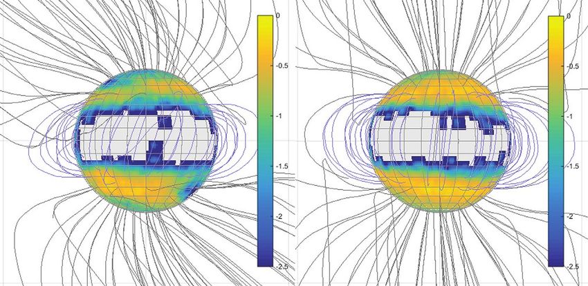
C. Plainaki et al.: Scientific aspects and future perspectives of planetary space weather

exist for Earth, followed by Saturn, Jupiter and Mercury                the Solar System is particularly challenging and requires as a
(Krupp 2015), whereas important information has also been               first step the definition of key observable quantities. With this
obtained from ground-based or Earth-orbiting telescopes as              in mind, it is clear that there is a strong need for detailed space
well as analytical and numerical models. The variability of             weather studies of individual planetary environments. In sum-
the spacecraft radiation environment due to major space                 mary, the planetary space weather discipline aims at:
weather events has often resulted in either a partial or a
complete failure of the detection systems on board. One such               d   understanding the nature of planetary environments
example is the radiation detector of the Mars Radiation                        revealing the physics of their interactions with the solar
Environment Experiment (MARIE) on-board Mars Odyssey                           wind and/or the magnetospheric environments to which
(Andersen 2006), which was presumed to have failed due to                      they are embedded;
damage from the unusually intense SEP events of October–                   d   forecasting and nowcasting the space environment
November 2003. Another example involved the Nozomi space-                      variability around a body in the Solar System;
craft, which suffered disruptions to its communication system              d   predicting the impacts of space environments on
due to a solar flare occurring in April 2002 (Miyasaka et al.                  technological systems on-board spacecraft and/or even-
2003). Another major space weather event resulted in an                        tually on humans.
increase in background radiation that made it difficult for the
Analyser of Space Plasmas and Energetic Atoms 3                             The scope of this review paper is to integrate the effort
(ASPERA-3) instrument on-board Mars Express (MEX) to                    started in the earlier study by Lilensten et al. (2014) by
evaluate ion escape fluxes at Mars (Futaana et al. 2008). Due           (a) providing an update of the current knowledge on the
to these phenomena, there is an increasing need for an overall          scientific aspects of planetary space weather, with special
effort to understand, monitor and potentially predict (to the           emphasis on the outer Solar System; (b) discussing considera-
extent that the latter is possible) the actual conditions around        tions related to future missions such as ESA JUICE and ESA/
the planetary environment under investigation. In order to              JAXA BEPI COLOMBO and (c) demonstrating the benefit for
achieve the maximum benefit from such an effort, it is                  the circum-terrestrial space weather discipline from studies
necessary to extend the methodological frameworks of                    related to other planetary environments. In Section 2, we
circum-terrestrial space weather to different contexts.                 present a brief review of the interactions taking place at differ-
Therefore, the strongest motivation for the current scientific          ent Solar System bodies, demonstrating that a ‘‘general
review is the need for a synoptic organization of the available         approach’’ to the topic of planetary space weather cannot be
knowledge on the field of interactions at different planetary           easily adopted; in Sections 2.1 and 2.2 we review the outer
systems, in parallel with a comparative analysis encompassing           and inner Solar System cases, respectively. In Section 3,
the inter-connection among planetary space weather aspects              we discuss some aspects of space weather from a comparative
belonging to different disciplines (e.g. plasma variability and         planetology viewpoint and give some considerations related to
its effects on atmospheric heating).                                    the planning of future observations both with Earth-orbiting
     Among others, the future ESA JUpiter ICy moons Explorer            telescopes and instruments on-board spacecraft at different
(JUICE) and the ESA/JAXA BEPI COLOMBO (composed of                      planetary environments. The importance of such investigations
two spacecraft in orbit around Mercury) space missions (to be           for the interpretation of in-situ observations is discussed
launched in 2022 and 2018, respectively) will provide the               extensively. Although in the current paper we focus on topics
opportunity to study space weather phenomena at two different           related to the upcoming missions ESA JUICE and ESA/JAXA
regions of our Solar System, dominated by essentially different         BEPI COLOMBO, we emphasize the relevance of such
conditions. Moreover, among the principal science objectives            planetary space weather studies for future missions to all
of JUICE are the investigation of the near-moon plasma and              destinations in the Solar System. In Section 4, we discuss
neutral environments as well as the characterization of Jupiter’s       the benefit from planetary space weather studies for the
atmosphere and magnetosphere (Grasset et al. 2013). In this             circum-terrestrial space weather research. The conclusions of
view, a synopsis of the plasma variability in the giant planet’s        this study are presented in Section 5. We underline that in
magnetosphere and its effects on the exospheres of the moons            the current paper, interactions between comets and their
and the atmosphere of the planet itself is a useful tool for any        external environment, as well as interactions at the Pluto-
related study; moreover, such an effort is rather urgent since it       Charon system have been intentionally omitted due to contin-
could be of help during the definition of the mission’s                 uous updates in these fields, provided by the ESA Rosetta and
observational strategies as well as during the implementation           NASA New Horizons missions, respectively.
of related models. Furthermore, the results acquired by the
Cassini mission have demonstrated that the plasma variability
in the Saturn system is an important agent in the interactions          2. Space weather interactions in the Solar System
within the planet’s magnetosphere and atmosphere as well as
in the moon and ring environments (André et al. 2008; Jia               The interactions of different Solar System bodies with solar
et al. 2010). The interactions between the Enceladus (Fleshman          wind and/or magnetospheric plasma have different spatial
et al. 2010) and possibly Europa (Roth et al. 2014a) plumes             scales and timescales. Moons can be submerged in their
with the magnetospheric environments are two other important            parent body’s magnetosphere either permanently (e.g.
examples of planetary space weather phenomena about which               Ganymede) or for a fraction of their orbit (e.g. Titan). In the
our knowledge is currently limited. In addition, the Uranus             Jupiter and the Saturn systems, the speed of the corotating
case is perhaps one of the most intriguing environments in              (with the planet) plasma is higher than the orbital velocity of
the outer Solar System for planetary space weather studies,             some satellites. As a result, the thermal corotating plasma over-
mainly due to the particular orientation of the solar wind              takes these moons. For example, the orbital speed of Enceladus
direction, relative to the planet’s rotation axis and magnetic          is 12.6 km/s while the thermal plasma corotates with Saturn at
field. The determination of the space weather conditions in             39 km/s near Enceladus and thus the corotating plasma

                                                                 A31-p3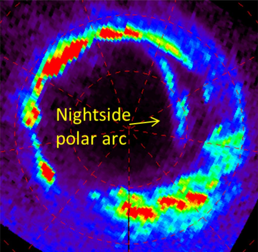
J. Space Weather Space Clim., 6, A31 (2016)

                      (a)                                                   (b)

                      (c)                                                   (d)

Fig. 1. Comparison of the sizes of magnetospheres of the outer planets, the Earth and Mercury. Boxes illustrate the relative size of the
magnetospheres. The conical at the left of each planet represents the bow shock, whereas the swept-back lines represent the planetary magnetic
field. (a) Mercury. (b) The Earth. (c) Saturn (left) and Jupiter (right). (d) Uranus or Neptune. Adapted from Kivelson & Russell (1995).

overtakes this moon forming a ‘‘corotational wake’’ at the                because the equatorial region is shielded from electrons over
hemisphere leading the moon’s orbital motion. The Cassini                 all longitudes, whereas in the leading sector, magnetic
Plasma Spectrometer (CAPS) registered a strong enhancement                reconnection (i.e. the breaking and topological rearrangement
in the flux of plasma ions when passing upstream of this wake.            of magnetic field lines in a plasma, resulting in the conversion
    In general, the interactions between Solar System bodies              of magnetic field energy to plasma kinetic and thermal energy)
and their space environment depend strongly on whether the                could lead to some sputtering of surface material at low
body is magnetized or unmagnetized. In Figure 1, the magne-               latitudes from recently trapped particles; in those regions,
tospheres of the four outer planets, the Earth and Mercury are            however, such a process is expected to have lower rates than
presented.                                                                in the polar caps. Recent simulations by Plainaki et al.
    A typical case study for the outer Solar System is Jupiter            (2015) of Ganymede’s sputter-induced water exosphere support
and its moons Europa, a satellite without any intrinsic                   this scenario. In contrast to Ganymede, the entire surface of
magnetic field, and Ganymede, not only the largest moon but               Europa is bombarded by Jovian plasma (maximum precipitat-
also the only known satellite in the Solar System possessing              ing flux is at the trailing hemisphere apex), suggesting that
its own magnetosphere. Leading/trailing hemisphere albedo                 sputter-induced redistribution of water molecules is a viable
and colour ratio asymmetries have been previously reported                means of brightening the satellite’s surface. As a consequence
for both Ganymede (Clark et al. 1986; Calvin et al. 1995)                 of these space weather conditions at Europa, the spatial
and more significantly for Europa (McEwen 1986; Sack                      distribution of the generated H2O exosphere is expected to
et al. 1992). For Ganymede, the leading hemisphere has a                  follow the pattern of the ion precipitation to the surface, being
measurably higher ratio in the green/violet colour ratio                  most intense above the moon’s trailing hemisphere (see
(0.79) than the trailing hemisphere (0.73), implying a                  Plainaki et al. 2012, 2013). On the basis of the above paradigm,
greater abundance of fine-grained frost on the leading                    it becomes clear that a ‘‘general approach’’ to the topic of
hemisphere. Additionally, images of Ganymede acquired by                  planetary space weather, determined by the interactions
Voyager 2 revealed that Ganymede’s high-latitude regions are              between the body’s environment and its surrounding space, is
noticeably brighter than its equatorial regions (Smith et al.             not straightforward.
1979). Khurana et al. (2007) showed that there is a clear link
between plasma bombardment and polar cap brightening at                   2.1. Space weather in the outer Solar System
Ganymede and suggested that sputter-induced redistribution
and subsequent cold trapping of water molecules is responsible            All planets in the outer Solar System possess magnetic fields,
for the observed bright and dark patches of the bright polar              which can be assumed to have approximately either a dipole
terrain. These authors also suggested that leading vs. trailing           form (e.g. Jupiter and Saturn, with tilt angles 9.6 and 0,
brightness differences in Ganymede’s low-latitude surface are             respectively) or a multipole form (e.g. Uranus and Neptune,
due to enhanced plasma flux onto the leading hemisphere,                  with tilt angles 59 and 47, respectively). Space weather at
rather than to darkening of the trailing hemisphere. This is              the environments of the outer planets depends on one hand

                                                                   A31-p4
C. Plainaki et al.: Scientific aspects and future perspectives of planetary space weather

on the solar wind density and the IMF intensity and direction,              (a)
and on the other hand on the planetary magnetic field tilt and
plasma pressure inside the magnetosphere. Below we will
discuss the different characteristics of these magnetospheres
related to space weather.

2.1.1. Space weather at Uranus, Neptune and exoplanetary
       analogues

Neptune and Uranus have strong non-axial multipolar magnetic
field components compared with the axial dipole component
(Connerney et al. 1991; Herbert 2009). These highly non-
symmetric internal magnetic fields (Ness et al. 1986, 1989;
Connerney et al. 1991; Guervilly et al. 2012), coupled with
the relatively fast planetary rotation and the unusual inclination
of the rotation axes from the orbital planes, imply that the                (b)
magnetospheres of Uranus and Neptune are subject to drastic
geometrical variations on both diurnal and seasonal
timescales. The relative orientations of the planetary spin, the
magnetic dipole axes and the direction of the solar wind flow
determine the configuration of each magnetosphere and, conse-
quently, the plasma dynamics. Space weather phenomena,
therefore, at these environments are expected to be signifi-
cantly variable in intensity and morphology over a range of
timescales. The study of the interactions responsible for space
weather phenomena at the environments of the icy giants
can also be used as a template for exoplanetary investigations.
     On the basis of the Voyager 2 occultation measurements,
the atmosphere of Uranus up to the vicinity of the exobase               Fig. 2. (a) Abundance and temperature profiles of the main
(i.e. near ~1.25 RU, where RU is the planet’s radius) consists           constituents of Uranus upper atmosphere, as inferred from the
mainly of H2 (Herbert et al. 1987). At higher altitudes, atomic          occultation observations by the Voyager 2 ultraviolet spectrometer.
H becomes the major constituent. The Voyager IR spectrometer             Helium was not detectable in the occultations hence it has been
deduced also a He content of about 15% (see Fig. 2). At the              extrapolated upwards from IRIS measurements (Hanel et al. 1986).
current moment, our knowledge on space weather phenomena                 From Herbert et al. (1987). (b) Modelled ionospheric profiles of
at Uranus is essentially based on (a) a limited set of plasma,           electron densities for Uranus using the Voyager inferred tempera-
FUV and IR measurements obtained during the Voyager 2 flyby              ture profiles. From Waite & Cravens (1987).
(Herbert 2009), (b) a series of observations of the FUV and IR
aurora with the Hubble Space Telescope (HST; Ballester 1998)
and (c) observations from ground-based telescopes (e.g.                  reconnection sites, the details of the solar wind plasma entry
Trafton et al. 1999). Voyager 2 provided a single snapshot of            in the inner magnetosphere of Uranus, the plasma precipitation
the Uranian magnetosphere at solstice, when the angle of attack          to the exosphere and ionosphere, the modes of interaction
between the solar wind axis and the magnetic dipole axis varied          (pickup, sputtering and charge exchange) between the magne-
between 68 and 52, to some extent similar to the situation at          tospheric plasma and the rings and moons of Uranus are
the Earth’s magnetosphere (Arridge et al. 2014). Moreover, the           largely unknown. Proton and electron radiation belts (with
Voyager 2 plasma observations showed that when the Uranus                energies up to tens of MeVs), albeit slightly less intense than
dipole field is oppositely directed to the interplanetary field,         those at Saturn, were also observed in the inner magnetosphere
magnetic plasma injection events are present in the inner                of Uranus (Cheng et al. 1991; Mauk & Fox 2010) but their
magnetosphere, likely driven by reconnection every planetary             diurnal and seasonal variability is also unknown to a great
rotation period (Sittler et al. 1987). However, the near                 extent (Arridge et al. 2014). Recent observations and theoreti-
alignment of the rotation axis with the planet-Sun line during           cal works on this thematic suggest a limited role for the solar
solstice means that plasma motions produced by the rotation              wind-driven dynamics at equinox (Lamy et al. 2012; Cowley
of the planet and by the solar wind are effectively decoupled            2013) and solar wind-magnetosphere coupling via magnetic
(Selesnick & Richardson 1986; Vasyliunas 1986) hence the                 reconnection that varies strongly with season and solar cycles
related space weather phenomena are expected to differ                   (Masters 2014). At the moment, therefore, it is not clear if
substantially from those at Earth, both in timescales and spatial        space weather phenomena are determined predominantly by
morphology. Due to the planet’s large obliquity, near equinox,           solar wind or by a more rotation-dominated magnetosphere,
Uranus’ asymmetric magnetosphere changes between near-                   such as the one at Jupiter or Saturn (Arridge et al. 2014).
pole-on and near-perpendicular configurations, every quarter             Future missions to Uranus with the science goal, among others,
of a planetary rotation. The configuration of Uranus’ magneto-           to understand the solar wind-magnetosphere-ionosphere
sphere in the 2030s is shown in Figure 3.                                coupling and its role in determining the space weather condi-
     The available in-situ measurements of space weather-                tions at the icy giant, have been recently proposed (Arridge
related interactions in the Uranian system refer to a single             et al. 2012, 2014; Turrini et al. 2014).
configuration between the planet and the solar wind flow.                    The aurora of Uranus is perhaps the most significant
Therefore, the time-dependent modulation of the magnetic                 evidence of how space weather conditions around the planet

                                                                  A31-p5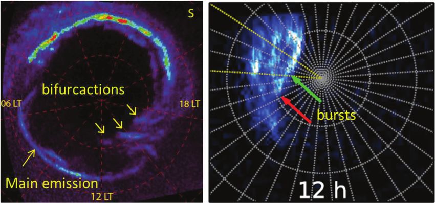
J. Space Weather Space Clim., 6, A31 (2016)

    (a)                                                                   other spectra except for those corresponding to November
                                                                          2011. Future in-situ plasma and energetic neutral particle
                                                                          observations could provide significant feedback for the
                                                                          determination of the planet’s space weather conditions and
                                                                          for determining if they indeed have a key role in this context.
                                                                          The planetary period modulation of the field-aligned currents
                                                                          at Uranus may lead to modulated auroral electron acceleration
                                                                          in regions of upward currents, as it happens in the case of
                                                                          Saturn (e.g., Nichols et al. 2008, 2010a, 2010b; Southwood
                                                                          & Kivelson 2009; Badman et al. 2012; Hunt et al. 2014);
                                                                          associated modulated radio emissions at kilometre wavelengths
                                                                          generated via the cyclotron maser instability could be present
                                                                          (Zarka 1998; Lamy et al. 2010, 2011). Such observations can
                                                                          be essential for the identification of space weather phenomena
                                                                          at Uranus.
                                                                              An additional particle source, at least in the inner
                                                                          magnetosphere of Uranus, may be the Cosmic Ray Albedo
                                                                          Neutron Decay (CRAND), responsible for the MeV ion spectra
                                                                          changes as a function of dipole L, where L is the McIlwain
                                                                          parameter4 (Krupp 2015). The CRAND source has also been
    (b)                                                                   suggested and confirmed to be a source for both Jupiter’s
                                                                          (Bolton et al. 2015) and Saturn’s radiation belts (Kollmann
                                                                          et al. 2013). Given the variability of the magnetosphere config-
                                                                          uration at Uranus, the CRAND source may have a significant
                                                                          role in determining the space weather conditions around the
                                                                          planet, especially in the inner magnetosphere regions.
                                                                              The magnetospheric interaction with the Uranian moons
                                                                          and rings, basically unknown at the current moment, is the
                                                                          agent of space weather at these systems. However, the Voyager
                                                                          data did not provide any evidence for such phenomena. Space
                                                                          weather phenomena occurring due to coupling between the
                                                                          planet’s magnetosphere and the expected tenuous atmospheres
                                                                          around the Uranian moons and rings could be identified and
                                                                          studied through in-situ measurements of magnetic field,
                                                                          charged particles and surface-released neutrals. Moreover,
                                                                          remote imaging of charge-exchange energetic neutral atoms
                                                                          (ENAs) would offer a unique opportunity to monitor the
                                                                          plasma circulation where moons and/or Uranus’ exosphere
                                                                          are present (Turrini et al. 2014). However, Krupp (2015)
                                                                          noticed that the highly variable inclination of the Uranian
Fig. 3. The magnetosphere of Uranus in the late 2030s between             moons with respect to the magnetic equator of the planet could
solstice and equinox where the rotation axis has a significant out-of-    lead to highly variable interactions between magnetospheric
plane component. Planetary rotation results in significantly different    populations and moon surfaces. In this case, water particles
magnetosphere configurations. The angle between the magnetic              could be sputtered and hence contribute to the magnetospheric
dipole vector (red arrow) and the planet’s rotational plane is ~59.      population once they get ionized, determining the space
Credit: Chris Arridge, Fran Bagenal and Steve Bartlett.
                                                                          weather conditions in the moons’ vicinity.
                                                                              Neptune is a relatively weak source of auroral emissions at
vary. It is underlined that one of the major open questions               UV and radio wavelengths (Broadfoot et al. 1989; Bishop et al.
regarding Uranus is the determination of the exact mechanism              1995; Zarka et al. 1995, Zarka 1998). Although this non-
providing the required additional heating of the planet’s upper           observation does not rule out an active magnetosphere, it rules
atmosphere. In a recent study, Barthelemy et al. (2014)                   out processes similar to those associated with the aurora
analysed HST FUV spectral images obtained in November                     observed at Uranus. Whereas the plasma in the magnetosphere
2011 (Lamy et al. 2012) and in 2012, with the scope to extract            of Uranus has a relatively low density and is thought to be pri-
any possible H2 emission produced in the upper atmosphere of              marily of solar wind origin, at Neptune, the distribution of
the planet. For their interpretations of the data, they used              plasma is generally interpreted as indicating that Triton is a
simulated H2 emissions created by energetic particle precipita-           major source (Belcher et al. 1989; Krimigis et al. 1989; Mauk
tion in the upper atmosphere. They found that for the spectrum            et al. 1991, 1995; Richardson et al. 1991). Neptune’s satellite
of November 2011, when an auroral spot was positively                     Triton, the largest of the 14 known Neptunian moons,
detected, a small contribution of H2 emission was identified              possesses a nitrogen and methane atmosphere with a surface
providing, hence, evidence for the presence of precipitating              pressure of 14 microbar and temperature of about 35.6 K,
electrons, giving a total energy input of at least 150 GW.
In the context of space weather, it is important to note that                 4
                                                                             The L-shell or McIlwain parameter describes the set of magnetic
Barthelemy et al. (2014) did not find any evidence for auroral            field lines which cross the planet’s magnetic equator at the distance
electron-induced emission above the detection threshold in any            of a number of planetary radii equal to the L-value.

                                                                     A31-p6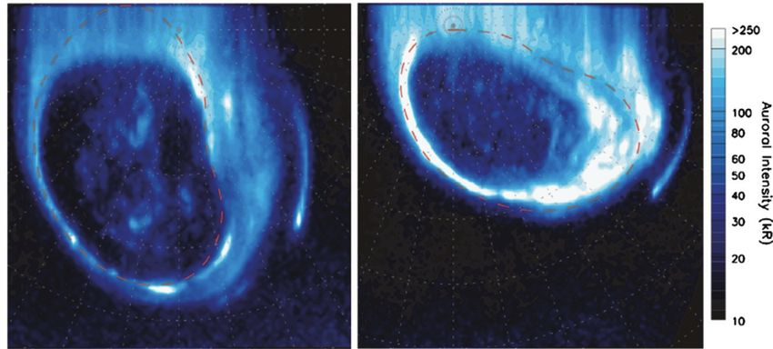
C. Plainaki et al.: Scientific aspects and future perspectives of planetary space weather

extending to 950 km above the surface. The exosphere temper-
ature reaches 95 K (Coustenis et al. 2010). Most of the
atmosphere contains a diffuse haze, which probably consists
of hydrocarbons and nitriles produced by the photolysis of
N2 and CH4 (McKinnon & Kirk 2007). Therefore, space
weather at Neptune could be substantially the result of the
interaction between Triton-originating plasma and Neptune’s
magnetosphere and atmosphere systems. It is underlined that
escape of neutral hydrogen and nitrogen from Triton maintains
a large neutral cloud (Triton torus) that is believed to be source
of neutral hydrogen and nitrogen (Decker & Cheng 1994).
The escape of neutrals from Triton could be an additional
plasma source for Neptune’s magnetosphere (through ioniza-
tion). An agent for possible space weather phenomena at
Triton’s vicinity is possibly the presence of active geysers, a
source of ions for the whole system, similar to the one at               Fig. 4. Density profiles of various components of Saturn’s upper
Saturn’s moon Enceladus (Porco et al. 2014). Since our                   atmosphere obtained from forward modelling of the Cassini UVIS
knowledge of the plasma dynamics in the magnetosphere of                 d-Ori stellar occultation on 2005 DOY 103 at a latitude of 42.7.
Neptune as well as on the neutral particle production in Triton’s        From the book Saturn from Cassini-Huygens (M.K. Dougherty et al.
atmosphere is limited (it is based only on a single flyby by             eds.), Chapter 8 by Nagy et al. (2009).
Voyager 2 in 1989), new in-situ plasma and energetic neutral
particle observations focused on Triton’s region could be of
particular importance for future studies related to planetary
space weather in the outer Solar System. Space weather
phenomena at Neptune’s moons depend on combined effects
of photoionization, electron impact ionization and charge
exchange in the context of a complex coupling between an
asymmetric planetary magnetosphere and satellite exospheres
at large distances from the Sun.

2.1.2. Space weather in the Saturnian system

Saturn is the second largest planet in our Solar System, follow-
ing Jupiter. Similar to the Jovian case, Saturn is a fast rotating
system, with a rotation of approximately 10.5 h (Gombosi
et al. 2009). Above the homopause, H2, H and He dominate
the upper atmosphere (see Fig. 4). Space weather at Saturn
is manifested by the occurrence of aurorae and thermospheric
emissions providing insights into the state of the planet’s
thermosphere and ionosphere (Fig. 5).
    The interaction of Saturn’s magnetic field with the solar
wind generates a giant magnetosphere which is dynamically
and chemically coupled to all other components of Saturn’s
environment: the rings, the exosphere, the icy satellites (and
their tenuous atmospheres), the Enceladus’ plumes and Titan’s
upper atmosphere. It is thus dominated by numerous
interactions between charged particles, neutral gas and dust
in addition to the usual interactions with the solar wind (Blanc         Fig. 5. Noon ion density profiles at Saturn. From the book Saturn
et al. 2002). Saturn’s magnetosphere is believed to be an                from Cassini-Huygens (M.K. Dougherty et al. eds.), Chapter 8 by
intermediate case between the magnetosphere of the Earth                 Nagy et al. (2009).
and the one of Jupiter (Andriopoulou et al. 2014). A unique
feature is that it is neutral-dominated. The neutral-to-ion ratio
is roughly 60, for radial distances ranging from 3 Rs to 5 Rs            et al. 2006) and the planet’s thermosphere (Shemansky et al.
(with Rs being Saturn’s radius). This ratio increases for larger         2009) can be additional sources supplying neutrals in Saturn’s
and smaller distances (Mauk et al. 2009; Melin et al. 2009;              magnetosphere. Indeed, a ‘‘ring ionosphere’’ was detected by
Shemansky et al. 2009). The density profiles of H2O and                  the CAPS instrument on-board Cassini (Coates et al. 2005).
atomic H peak near the Enceladus orbit at a distance of                      The investigation of the magnetopause reconnection driven
~3.95 Rs from the planet (Perry et al. 2010). Other Saturnian            by the solar wind started in the Voyager era. However, its
satellites residing in the planet’s magnetosphere can act both           significance is a subject of large debate to date. Voyager
as plasma sinks and sources. Observations from early flyby               observations showed reconnection signatures at Saturn’s
missions to Saturn revealed a very complex ring system with              magnetopause (Huddleston et al. 1997) and suggested that
several gaps, where the energetic particle density drops, mainly         bursty reconnection similar to flux transfer events at Earth
due to the satellites’ presence. The ring system itself (Johnson         (Russell & Elphic 1979) is not a significant mechanism at

                                                                  A31-p7
J. Space Weather Space Clim., 6, A31 (2016)

Saturn, because of the high magnetosonic Mach numbers5               arcs are related to bursty reconnections at Saturn involving
which are reached close to Saturn. On the other hand, Cassini        upward field-aligned currents (Badman et al. 2012) and
plasma and magnetic field observations revealed signatures of        suggested that these are efficient in transporting flux (Badman
reconnection at Saturn’s magnetopause (McAndrews et al.              et al. 2013). A more recent study based on conjugated IMF and
2008). Recently, it was suggested that only a limited fraction       HST observations (Meredith et al. 2014) provided evidence of
of the magnetopause surface could become open (Masters               significant IMF dependence on the morphology of Saturn’s
et al. 2012). Moreover, recent studies indicated that reconnec-      dayside auroras and the bifurcated arcs. Finally, the auroral
tion has a less important role at Saturn than at the Earth, in       evidence of magnetopause reconnection at multiple sites along
large-scale transport near the subsolar region of the magne-         the same magnetic flux tube similar to the terrestrial case
topause (Lai et al. 2012). Finally, several auroral studies          (Fasel et al. 1993) was shown to give rise to successive
provide evidence for the importance of solar wind driven             rebrightenings of auroral structures (Radioti et al. 2013b).
reconnection at Saturn’s magnetopause (see among others              The same auroral features, together with magnetospheric
Badman et al. 2011; Radioti et al. 2011b; Jasinski et al.            measurements, were discussed in Jasinski et al. (2014) in terms
2014; Meredith et al. 2014).                                         of cusp signatures at Saturn’s high-latitude magnetosphere.
                                                                          However, it should be noted that the significance of magne-
2.1.2.1. Solar wind effects on the aurora                            topause reconnection at Saturn is under debate (Masters et al.
The main auroral emission at Saturn (Fig. 6) can be associated       2012). Alternatively to solar wind driven reconnection, the
with the solar wind-magnetosphere interaction through the            viscous interaction of the solar wind with the planetary
generation of field-aligned currents and plasma precipitation        magnetosphere, which involves magnetic reconnection on a
(e.g. Cowley et al. 2004), similar to the terrestrial aurora         small scale (Delamere & Bagenal 2013), influences Saturn’s
(e.g. Paschmann et al. 2002). Particularly, Cassini measure-         magnetopause dynamics. Cassini UVIS observations revealed
ments in comparison with conjugated auroral observations             recently the presence of small-scale structures in the dayside
suggest that the main auroral emission at Saturn is produced         main auroral emissions indicative of magnetopause Kelvin-
by the magnetosphere-solar wind interaction, through the shear       Helmholtz instabilities, which are key elements of the solar
in rotational flow across the open-closed field line boundary        wind-magnetosphere viscous interaction (Grodent et al. 2011).
(OCFB; e.g. Cowley & Bunce 2001; Bunce et al. 2008). The                  In addition to dayside magnetopause, the solar wind
morphology of Saturn’s aurora is demonstrated to respond to          influences Saturn’s magnetotail and this interaction leaves its
solar wind changes (Grodent et al. 2005; Clarke et al. 2009),        footprint in the aurora. It has been suggested that Saturn’s
controlled by the balance between the magnetic field reconnec-       magnetotail is influenced by a combination of solar wind
tion rate at the dayside magnetopause and the reconnection rate      (Dungey 1961, like at Earth) and internally driven magnetic
in the nightside tail (Cowley et al. 2004; Badman et al. 2005,       reconnection (Vasyliunas 1983) as well as viscous interaction
2014).                                                               of the solar wind with the planetary magnetosphere (Delamere
    HST observations (Gérard et al. 2004, 2005) and theoreti-        & Bagenal 2013). Tail reconnection in the Dungey-cycle
cal studies (Bunce et al. 2005) showed that reconnection             manner is expected to result in bright and fast rotating aurorae,
occurring at the dayside magnetopause could give rise to bright      which expand poleward in the dawn sector, reducing
UV auroral emissions at Saturn observed occasionally near            significantly the size of the polar cap and thus resulting in
noon, similar to the ‘‘lobe cusp spot’’ at Earth (i.e. emissions     the closure of flux (Badman et al. 2005; Cowley et al. 2005;
located at the cusp magnetic foot point, Fuselier et al. 2002).      Jia et al. 2012).
The magnetospheric ‘‘cusp’’ is the magnetospheric region                  Particularly, intense auroral activity in the dawn auroral
where magnetosheath plasma has direct access to the iono-            sector was recently observed by Cassini/UVIS and was
sphere through reconnection. Specifically, it was proposed by        characterized by significant flux closure with a rate ranging
Bunce et al. (2005) that pulsed reconnection at the low-latitude     from 200 to 1000 kV (Radioti et al. 2014). Additionally,
dayside magnetopause for northward-directed IMF is giving            Nichols et al. (2014) based on HST observations revealed
rise to pulsed twin-vortical flows in the magnetosphere and          auroral intensifications in the dawn auroral sector, propagating
ionosphere in the vicinity of the OCFB lines. For the case of        at 3.3 times the rigid corotation. These intensifications were
southward IMF and high-latitude lobe reconnection, bipolar           suggested to be indicative of ongoing, bursty reconnection of
field-aligned currents are expected, associated with auroral         lobe flux in the magnetotail, with flux closure rates of
intensifications poleward of the OCFB lines.                         280 kV (Fig. 6b). Badman et al. (2015) reported an event of
    Cassini Ultraviolet Imaging Spectrograph (UVIS) auroral          solar wind compression that impacted Saturn’s magnetosphere,
observations revealed signatures of consecutive reconnection         identified by an intensification, and extension to lower
events at Saturn’s magnetopause (Radioti et al. 2011b) in the        frequencies, of the Saturn kilometric radiation. This event
form of bifurcations of the main emission (Fig. 6a). In the          was manifested in the auroral dawn region as a localized
same study it was suggested that magnetopause reconnection           intense bulge of emission followed by contraction of the night-
could lead to a significant increase of the open flux within a       side aurora. These observations are interpreted as the response
couple of days. In particular, each reconnection event is            to tail reconnection events, initially involving Vasyliunas-type
estimated to open 10% of the flux contained within the polar        reconnection of closed mass-loaded magnetotail field lines,
cap. Additionally, Cassini multi-instrument observations,            and then proceeding onto open lobe field lines, causing the
including auroral UV and IR data, confirmed that the auroral         contraction of the polar cap region on the nightside.
                                                                     Additionally, Radioti et al. (2016) revealed multiple intensifica-
5
  The magnetosonic Mach number, Mf, is defined as the upstream       tions within an enhanced auroral dawn region suggesting an
(with respect to a collisionless shock) flow speed divided by the    x-line in the tail, which extends from 2 to 5 LT. Such UV inten-
speed of the fast magnetosonic wave, which steepens to form the      sifications have been also previously suggested to be associated
shock (Masters et al. 2011). Mf is always >1 for shocks, by          with depolarizations in the tail (Jackman et al. 2013). The local-
definition.                                                          ized enhancements reported by Radioti et al. (2016) evolved
                                                                A31-p8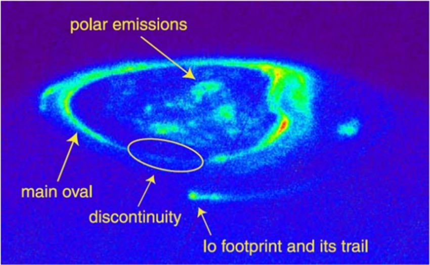
C. Plainaki et al.: Scientific aspects and future perspectives of planetary space weather

                       (a)                                             (b)

Fig. 6. (a) Polar projection of Saturn’s southern aurora obtained with the FUV channel of UVIS on-board Cassini on DOY 21, 2009. Noon is to
the bottom and dusk to the right. The grid shows latitudes at intervals of 10 and meridians of 40. Arrows indicate the main emission and the
bifurcations of the main auroral emission. Adapted from Radioti et al. (2011b). (b) Polar projection of Saturn’s aurora obtained with the HST on
day 95, 2013. Noon is to the bottom and dusk to the right. A grey 10 · 10 latitude-longitude grid is overlaid. Arrows show bursts of
emissions indicative of reconnection of lobe flux in the magnetotail. Adapted from Nichols et al. (2014).

in arc and spot-like small-scale features. They are likely related
to plasma flows enhanced from reconnection, which diverge
into multiple narrow channels and then spread azimuthally
and radially. The evolution of tail reconnection at Saturn
may be illustrated by an ensemble of numerous narrow current
wedges or inward transport initiated in the reconnection region,
likely explained by multiple localized flow burst events.
    Enhancements in ENA emission and Saturn kilometric
radiation data, together with auroral observations from HST
and UVIS, reported the initiation of several acceleration events
in the midnight to dawn quadrant, at radial distances in the
range from 15 Rs to 20 Rs, related to tail reconnection
(Mitchell et al. 2009). The formation of ENA emission is
discussed in Section 2.1.2.2. Numerical simulations together
with simultaneous UV and ENA emissions (Radioti et al.
2009a, 2013a) demonstrated that injected plasma populations
can create auroral emissions at Saturn, by pitch angle diffusion
associated with electron scattering by whistler-mode waves,
while field-aligned currents driven by the pressure gradient
along the boundaries of the cloud might have a smaller
contribution.
                                                                             Fig. 7. Polar projection of Saturn’s aurora as captured from UVIS
    Recently, UVIS auroral observations revealed the first and
                                                                             on-board Cassini on DOY 224, 2008. Noon is to the bottom and
only observation of an Earth-like transpolar arc at Saturn                   dusk to the right. The arrow indicates the first observation of an
(Fig. 7) (Radioti et al. 2014). At Earth, transpolar arcs are                Earth-like transpolar arc at Saturn. The formation of the nightside
auroral features, which extend from the nightside auroral oval               polar arc at Saturn may be related to tail reconnection. Adapted
into the open magnetic field line region (polar cap) and they                from Radioti et al. (2014).
represent the optical signatures of magnetotail dynamics (e.g.
Frank et al. 1982; Milan et al. 2005). The formation of the
nightside polar arc at Saturn may be related to solar wind                   Pioneer 11, Voyager 1 and 2 flyby missions (Van Allen
driven tail reconnection similarly to the terrestrial case (Milan            1983, 1984). The Cassini spacecraft arrived at Saturn in
et al. 2005). However, the rarity of the occurrence of the                   2004 and it has since then been providing extensive data on
transpolar arc at Saturn indicates that the conditions for its               the Kronian system and the radiation belts in particular.
formation are rarely met at the giant planet, contrary to the                    The energy range of Saturn’s charged particle population in
Earth.                                                                       the radiation belts is between some hundreds of keV up to tens
                                                                             of MeV, while the radial extent of this magnetospheric region
2.1.2.2. Space weather at the radiation belts                                is between 2.3 Rs up to 6 Rs approximately (Gombosi et al.
The radiation belt environments of the outer planets are quite               2009; Kollmann et al. 2013). Figure 8 shows the typical phase
different from the one of the Earth, mainly due to the presence              space density profiles of protons in the Kronian radiation belts
of moons and rings embedded in these systems. At Saturn, they                as a function of L-shell for several energy channels. Moving
were firstly explored using in-situ measurements from the                    inside 2.3 Rs, almost all the energetic particle population is

                                                                     A31-p9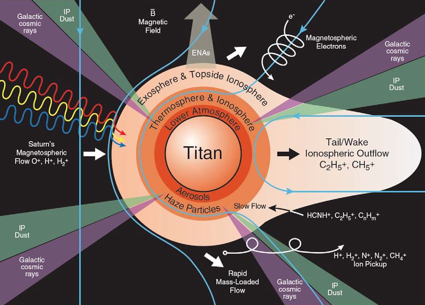
J. Space Weather Space Clim., 6, A31 (2016)

                                                                       Fig. 9. Schematic of the charge-exchange/stripping process that
                                                                       begins as ENA emission from the main belt populates the innermost
                                                                       radiation belt (‘‘new radiation belt’’) and ultimately produces ENA
                                                                       emission from Saturn’s exosphere. From Krimigis et al. (2005).

                                                                       2010). The most important source of the radiation belt protons
                                                                       with energies >10 MeV is the GCR population interacting with
                                                                       Saturn’s atmosphere and rings through the CRAND process
                                                                       (Blake et al. 1983; Cooper 1983; Kollmann et al. 2013) (see
                                                                       also Sect. 2.1.1). Such a mechanism has an important role also
                                                                       at the Earth’s radiation belts (Singer 1958). The CRAND
Fig. 8. Mission-averaged phase space density profiles of protons in
                                                                       process is also responsible for the most energetic component
Saturn’s radiation belts. From Kollmann et al. (2013).                 (>10 MeV) of Saturn’s innermost radiation belt (Kotova
                                                                       et al. 2014). While the proton radiation belts are characterized
                                                                       by stability, this is not the case for the electron radiation belts
depleted due to the presence of the main rings. An exception           that are characterized by both complex temporal and spatial
may be the region inside the D-ring of Saturn, where, evidence         variations. Satellites orbiting within the magnetospheres of
of a tiny energetic particle trapping region has been reported         the giant planets are effective absorbers of trapped radiation,
(Krimigis et al. 2005). Its presence was inferred from the             forming the characteristic and dominant structure of the
detection of an ENA population by the MIMI/INCA during                 radiation belts (Selesnick 1993) including electron macro and
the first Cassini orbit. The origin of this particle population        micro signatures. The solar UV irradiance from the thermo-
is expected to be the main proton radiation belt, after the            sphere of Saturn and the solar wind are the most probable
occurrence of double charge-exchange processes with particles          sources to account for the long-term variability of the electron
of the Saturnian exosphere: these protons undergo a first              radiation belts (Roussos et al. 2014), suggesting that external
charge-exchange, where they are transformed into planet-               drivers play indeed an important role in Saturn’s magneto-
directed ENAs that can ‘‘overfly’’ the planetary rings, stripped       spheric dynamics.
off an electron upon entry in Saturn’s exosphere and finally               Several modelling studies have been performed to describe
trapped as ions (Fig. 9).                                              the electron radiation belts taking into account mainly the
    The icy moons that inhabit the main radiation belts                radial diffusion processes (Hood 1983, Santos-Costa et al.
continuously absorb energetic particles at their orbits,               2003). More recently, Lorenzato et al. (2012) adapted the
separating in this way the ionic radiation belts and producing         Salammbô three-dimensional physical radiation belt model
‘‘sweeping corridors’’ (Kollmann et al. 2013; Kotova et al.            for Saturn’s electron radiation belts (Santos-Costa et al.
2015). Due to the approximate alignment of the magnetic axis           2003). Apart from radial diffusion, this model considers other
with the rotation axis, the energetic particle losses due to           important physical processes governing radiation belt
the moons are expected to be much more pronounced                      dynamics, and in particular, wave-particle interactions and
than the ones in the other outer planets (Roussos et al.               losses due to the rings, the icy satellites and their exospheres
2007). As a result, solar wind does not influence the inner            (Lorenzato et al. 2012).
radiation belt environment, which is rather stable. However,
a new transient radiation belt was recently discovered near            2.1.2.3. Space weather at the Saturnian moons
Dione’s orbit, at radial distances from 4.89 to 8 Rs approxi-          The plasma, magnetic field and neutral particles data obtained
mately (Roussos et al. 2008). This transient belt can be               since the arrival of the Cassini spacecraft at Saturn in July 2004
observed for up to a few weeks or months and its occurrence            have substantially enriched our knowledge of the magneto-
is related to periods of enhanced solar activity. It can be            sphere-satellite interactions determining the space weather
considered therefore as an evident manifestation of space              conditions at the giant planet’s moons. In the following para-
weather in the Saturnian system.                                       graphs we will focus on several of the moons of Saturn: Titan,
    Another mechanism for the energetic particle loss in the           the only known satellite with a dense nitrogen-dominated
Kronian radiation belts is the interaction of the ions with the        atmosphere, Rhea, Dione and Enceladus, a small icy moon
moons’ exospheres, and in particular with the exosphere and            identified as the major source of neutral particles and thus also
plumes of Enceladus (Tokar et al. 2006; Cassidy & Johnson              as source of magnetospheric plasma. Titan is located within

                                                                 A31-p10
C. Plainaki et al.: Scientific aspects and future perspectives of planetary space weather
Saturn’s magnetosphere for average solar wind conditions. The
orbital velocities of these moons are exceeded by the speed of
the (partially) corotating magnetospheric plasma. As a result,
they are continuously ‘‘overtaken’’ by the magnetospheric
plasma flow. The overall result of the interaction between
plasma and satellite depends both on the plasma conditions,
affected dynamically by internal plasma sources (e.g. neutral
gas from Enceladus), and on the properties of each satellite
itself (e.g. surface composition, endogenic neutral sources).
Space weather conditions at the locations of these moons
have been identified to some extent by the combination of
interdisciplinary measurements with Cassini, however
modelling and further investigation is necessary for resolv-
ing critical points to be taken into account during future
missions.
Fig. 10. The density profiles of N2, CH4, H2 and 40Ar, as obtained
Titan. Titan is the only other body, besides our own planet, to
from the Cassini/INMS measurements, averaged over all Cassini
have a dense atmosphere composed essentially of molecular flybys. The inbound (solid) and outbound (dashed) profiles are
nitrogen (~97%), and hosting an active and complex organic nearly identical, indicating that the wall effects are negligible for
chemistry created by the photolysis of methane (~2% in the these species. From Cui et al. (2009a).
stratosphere) and its interaction with nitrogen and hydrogen
(~0.1%). Figure 10 shows the density profiles of the main
components of Titan’s upper atmosphere, as obtained from source for this complex chemical factory in Titan’s upper
the Cassini Ion and Neutral Mass Spectrometer (INMS) atmosphere, and for creating an extended ionosphere.
measurements, averaged over all Cassini flybys. The reader Titan was found to have quite an extended ionosphere,
is requested to refer to Cui et al. (2009b, Fig. 9), for a descrip- between 700 and 2700 km, essentially due to the lack of a
tion of the observed diurnal variations of several representative strong intrinsic global magnetic field and the precipitation of
ion species in Titan’s ionosphere. energetic particles from Saturn’s magnetosphere. At lower
Adding to the Voyager 1 radio-occultation data, measure- altitudes, galactic cosmic rays are responsible for the produc-
ments by the Composite Infrared Radiometer Spectrometer tion of another ion layer in the atmosphere (between 40 and
(CIRS) on the orbiter and from the Huygens Atmospheric 140 km), while the neutral atmospheric photochemistry is
Structure Instrument (HASI) at the probe’s landing site mainly driven by FUV solar photons.
(10 S, 192 W) from 1400 km in altitude down to the surface Figure 11, adapted from Waite et al. (2004) and Sittler
allowed us to reconstruct the temperature structure of Titan. et al. (2009), shows schematically the main layers of Titan’s
A surface temperature of 93.65 ± 0.25 K was measured for a upper atmosphere, and their interaction with the energetic
pressure of 1467 ± 1 mbar (Fulchignoni et al. 2005). plasma flow from Saturn’s magnetosphere and the other energy
As revealed previously through Voyager data analysis, Titan’s sources. The direct analysis of the ionosphere by the INMS
atmosphere is composed (from upper altitudes to lower ones) instrument during the low-altitude Cassini flybys of Titan
of an exosphere, a thermosphere, a mesosphere, a stratosphere shows the presence of many organic species at detectable
and a troposphere, with two major temperature inversions at levels, in spite of the very high altitude (1100–1300 km).
40 and 250 km, corresponding to the tropopause and The interpretation of INMS measurements (limited to masses
stratopause, associated with temperatures of 70.43 K (min) up to 100 Daltons) and of Cassini/CAPS data (Coates et al.
and 186 K (max). A mesopause was also found at 490 km 2007, 2009) strongly suggests that high molecular weight
(with 152 K) in the early years of the Cassini mission, but species (up to several 1000 Daltons) may be present in the
has gradually disappeared in the recent years, leading to a more ionosphere (Waite et al. 2007, Fig. 7). Models applied to the
homogeneous vertical structure. The Voyager 1 UVS experi- data have pointed to the presence of complex molecules (see
ment had also recorded a temperature of 186 ± 20 K at Tables 6.2 and 6.4 in Coustenis & Taylor 2008). The vertical
1265 km during a solar occultation for a methane mixing ratio distributions of the trace gases increase with altitude, confirm-
of 8 ± 3% toward 1125 km, placing the homopause level at ing that these species form in the upper atmosphere and then
around 925 ± 70 km. diffuse downward in the stratosphere. Among the trace species
The Cassini-Huygens mission demonstrated that Titan’s detected to date we find hydrocarbons (C2H2, C2H4, C2H6,
atmosphere is a chemical factory in which the formation of C3H4, C3H8, etc.) and nitriles (HCN, HC3N, C2N2, etc.).
complex positive and negative ions is initiated in the high ther- Oxygen compounds such as H2O, CO and CO2 have also been
mosphere as a consequence of magnetospheric-ionospheric- detected.
atmospheric interactions involving solar EUV, UV radiation, The Cassini-Huygens measurements have revolutionized
energetic ions and electrons (Waite et al. 2005). Indeed, besides our perception of the organic processes occurring in Titan’s
the mother molecules, molecular nitrogen and methane, atmosphere, bringing forward a strong implication of the
a diverse host of neutral components was discovered in the ionospheric chemistry in the formation of complex organic
middle atmosphere, originating in the upper layers. compounds in Titan’s environment and acting as seed particles
Table 1 (from Sittler et al. 2009) summarizes the main for the formation of tholin material and haze. These
energy sources for Titan’s upper atmosphere. As shown, compounds are detectable in solar and stellar UV occultations
energetic particles from Saturn’s magnetosphere are, in addi- and initiate the process of haze formation (Waite et al. 2007) to
tion to UV and EUV radiation, the most important energy finally condense out starting at ~950 km (Fig. 12). As the haze
A31-p11You can also read